| Issue |
A&A
Volume 682, February 2024
|
|
|---|---|---|
| Article Number | A176 | |
| Number of page(s) | 8 | |
| Section | Stellar atmospheres | |
| DOI | https://doi.org/10.1051/0004-6361/202347901 | |
| Published online | 22 February 2024 | |
Unveiling the spectacular over 24-hour flare of star CD-36 3202
1
Astronomical Institute, University of Wrocław,
Kopernika 11,
51-622
Wrocław,
Poland
e-mail: This email address is being protected from spambots. You need JavaScript enabled to view it.
2
University of Wrocław, Centre of Scientific Excellence – Solar and Stellar Activity,
Kopernika 11,
51-622
Wrocław,
Poland
Received:
7
September
2023
Accepted:
24
November
2023
Abstract
We studied the light curve of the star CD-36 3202, which was observed by TESS for the presence of stellar spots and to analyze the rotationally modulated flare that took place on TESS Barycentric Julian Date 1486.93. Our main aims are to model the light curve of this flare and to estimate its location regarding stellar spots. The flare lasted approximately 27 h. Using our new tool, findinc_mc, we managed to estimate the inclination angle of the star to 70° ± 8°. With BASSMAN, we modeled the light curve of the CD-36 3202 and estimated that three spots are present on its surface. The mean temperature of the spots was about 4000 ± 765 K, and their total area amounted to 11.61% ± 0.13% on average. We created a new tool, named MFUEA, to model rotationally modulated flares, and used it to estimate the latitude of the long-duration flare event, finding 69−1+2 deg. Our estimation of the flare location is the first recreation of the exact position of a flare in relation to starspots. The flare is placed 12° from the center of the coolest spot. This means that the flare is related to the magnetic processes above the active region represented by the spot. Removing the effects of rotational modulation from the flare light curve allowed us to correct the estimation of bolometric energy released during the event from (1.15 ± 0.35) × 1035 erg to (3.99 ± 1.22) × 1035 erg.
Key words: magnetic fields / stars: activity / stars: flare / stars: late-type / stars: low-mass / starspots
© The Authors 2024
 Open Access article, published by EDP Sciences, under the terms of the Creative Commons Attribution License (https://creativecommons.org/licenses/by/4.0), which permits unrestricted use, distribution, and reproduction in any medium, provided the original work is properly cited.
This article is published in open access under the Subscribe to Open model. This email address is being protected from spambots. You need JavaScript enabled to view it. to support open access publication.
1 Introduction
In the vast expanse of the Universe, stars exhibit a fascinating array of behaviors and phenomena. Among these captivating features are starspots, stellar flares, and stellar activity, which provide insights into the dynamic nature of stars (Howard et al. 2019; Roettenbacher & Vida 2018). Stellar activity is an umbrella term used to describe the range of activities resulting from the interaction between a star’s magnetic field and its internal dynamics. Stellar activity is highly variable, with different stars exhibiting varying degrees of magnetic activity (Yang et al. 2017; Mathur et al. 2014). Younger stars, for instance, tend to be more active, displaying frequent flares and larger starspots, while older stars generally exhibit less activity (Davenport et al. 2019).
Starspots, which are referred to as sunspots when seen on the surface of the Sun, are dark, cooler regions that appear on the surface of stars (Biermann 1941; Hoyle 1949; Chitre 1963; Bray & Loughhead 1964; Deinzer 1965; Dicke 1970). These spots are caused by intense magnetic activity and can vary in size, shape, and duration. They are commonly found on stars that possess a convective envelope, where hot plasma rises from the interior, before cooling as it travels to the surface, and finally descending back into the star. The presence of starspots indicates the presence of strong magnetic fields on these stars, affecting their overall brightness and spectral characteristics (Flores et al. 2022).
Stellar flares are sudden and dramatic releases of magnetic energy in the form of intense bursts of electromagnetic radiation. Stellar flares are analogous to solar flares but can be significantly more powerful (Namekata et al. 2017; Pietras et al. 2022). They occur when the magnetic field lines of a star become twisted and tangled, leading to a rapid reconfiguration that releases tremendous amounts of energy. Stellar flares emit radiation across the electromagnetic spectrum, including X-rays and ultraviolet light, and can be detected by specialized observatories. These energetic events provide a glimpse into the violent and dynamic processes taking place within stars.
Understanding starspots, stellar flares, and stellar activity is crucial in order to comprehend the physical properties and evolutionary processes of stars. Through the study of these phenomena, we can gain insight into stellar magnetism, stellar winds, and the impact of stellar activity on planetary systems. Observing starspots and stellar flares on distant stars enables us to compare them to the Sun’s activity, and allows us to explore the broader context of stellar behavior and the potential habitability of exoplanets (Günther et al. 2020; Bogner et al. 2022).
Here, we present our analysis of the starspot distribution on CD-36 3202 and an analysis of the long-duration event (LDE) that occurred on that star on TBJD (TESS Barycentric Julian Date) 1486.93. We use light curves from TESS and compare the results of our analysis with previously published papers regarding starspot and flare activity for similar types of events and stars. We estimated the number of spots on this star and their parameters (temperature, size, stellar longitude, and latitude). We estimated the location of the flare and how it is arranged compared with the locations of the spots. In Sect. 2, we describe the star itself and in Sect. 3 we describe the observations. Our starspots modeling and flare analysis methods are provided in Sects. 4 and 5, respectively. Our results are presented in Sect. 6 and a discussion and conclusions are provided in Sect. 7.
2 CD-36 3202
We analyzed the variability of this star and the very interesting flare that took place on TBJD 1486.93. CD-36 3202 (also known as TIC156758257) is a partially convective K2V (Torres et al. 2006) young star of around 40 Myr of age (Bell et al. 2015) and is found at a distance of 90 pc. It has a radius of 0.8 R⊙, a mass of 0.8 M⊙, an effective temperature of 4885 K (MAST catalog1), and an estimated rotational period equal to 0.23536 ± 0.00046 days. In order to analyze the variability of this star, we estimated its inclination angle to be i = 70° ± 8° (for more details see Appendix A).
The flux level of the unspotted CD-36 3202 is needed in order to conduct a proper analysis of the distribution of starspots. We used the TESS observations from sector 7 due to the occurrence of the highest values of the star’s signal without any flares and used the methodology presented by Bicz et al. (2022) to evaluate this level, finding a value of 1.06053 in normalized flux (see the right side of Fig. 1).
Given the star’s flaring activity, rapid rotation period, and youthful age, we are attempting to explain the observed variability through the heightened spot activity on the star’s surface. This latter phenomenon is reflected in a notable alteration in luminosity, amounting to approximately 10%.
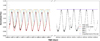 |
Fig. 1 TESS light curves from sectors 6 and 7, with a reconstructed starspot model and the unspotted stellar level highlighted. Left side: Part of the TESS light curve from sector 6 (black dots) during which the long-duration flare occurred, with the starspot model that recreates the curve (red line). The green, blue, and orange curves present the contribution of individual spots to the whole light curve. Right side: Part of the TESS light curve from sector 7 (black dots) with the estimated unspotted level of the star marked with a purple line. |
3 White-light data
In our investigation, we used data gathered from the TESS (The Transiting Exoplanet Survey Satellite; Ricker et al. 2014) mission. TESS, a space-based telescope, was launched in April 2018 and positioned in a highly elliptical orbit that completes a full cycle every 13.7 days. The primary objective of the mission is to provide uninterrupted observations of a significant portion of the celestial sphere, which is divided into 26 sectors. The satellite diligently monitors designated stars, employing a 2 min cadence (referred to as short cadence) and a 20 s cadence (known as fast cadence) throughout the approximately 27-day monitoring period in each sector. Additionally, using full frame images (FFIs), one can obtain light curves with a cadence of 30 min. In order to maintain consistency in our light-curve analysis, we specifically used the short-cadence light curves with the quality flag set to 0, ensuring that we are using the most accurate and reliable data.
4 Starspot modeling
We used BASSMAN2 (Best rAndom StarSpots Model cAlculatioN) presented by Bicz et al. (2022) to model starspots. BASSMAN recreates the light curve of a spotted star by fitting the spot(s) model – which is described by the amplitude, size, stellar longitude, and latitude of spot(s) – to the data. To do so, BASSMAN uses the Broyden–Fletcher–Goldfarb–Shanno (BFGS) algorithm (Fletcher 1987) and Markov chain Monte Carlo (MCMC) methods. The program uses the following ready-made software packages to model the spots on the star: starry Luger et al. (2019), PyMC3 Salvatier et al. (2016), exoplanet Foreman-Mackey et al. (2021), and theano Theano Development Team (2016). Each star is expressed in BASSMAN as a linear combination of spherical harmonics. The star is described by the vector of the spherical harmonic coefficients (indexed by increasing degree l and order m). Each starspot on the star is the spherical harmonic expansion of a Gaussian, with the assumption that the spot is spherical. It is worth mentioning that the starspots recreated by BASSMAN are not exactly sunspot-like structures. The software approximates an active region as one large spot, but in reality the region may consist of several individual spots and faculae. Due to the limitations of the method of reconstructing spots on the star’s surface, the actual active region, consisting of a series of spots and bright structures, cannot be obtained using single-passband photometry data.
5 Analysis of the flares
We used an automated, three-step software WARPFINDER (Wroclaw AlgoRithm Prepared For detectINg anD analyzing stEllar flaRes) – as presented by Bicz et al. (2022) and Pietras et al. (2022) – to analyze and detect flares on the light curve. The first step is the method based on consecutive detrending of the light curve described by Davenport et al. (2014). The second method of finding stellar flares is the Difference Method, which is based on Shibayama et al. (2013). The times from the lists of flare candidates created by both methods are compared and only the common detection in a designated time is treated by the software as a potential detection and passed on to the next level of verification. Then, the profiles of the assumed flares (Bicz et al. 2022; Pietras et al. 2022) are fitted to the observational data and the quality of these fits are checked with the χ2statistic. We use the probability density function (PDF) of the F-distribution to distinguish a stellar flare from noise in the data. Additionally, we calculate the skewness of the flare profile and check the bisectors of the profile in order to reject false detections. We assume that a stellar flare should have a shorter rise time than its decay time. We also reject all events with a duration of less than 6 observational points (12 min) for the short-cadence data and less than 18 observational points (6 min) for the fast-cadence data. WARPFINDER uses two methods to estimate the energy of a flare. The first is based on the method presented by Kovári et al. (2007) and the second is based on the method presented by Shibayama et al. (2013).
To estimate the possible location of a flare on the star and fit the theoretical flare profile proposed by Gryciuk et al. (2017), we created a new tool written in Rust named MFUEA3. MFUEA models the modulated flare using the differential evolution (DE) method. DE belongs to the category of evolutionary algorithms designed to address optimization problems with real-valued parameters. It serves as a highly effective method for black-box optimization, particularly when dealing with complex functions where finding the appropriate derivatives required to compute extreme values is challenging. DE takes inspiration from biological evolutionary processes, namely mutation, crossover, and selection. To achieve the desired solution, three crucial parameters come into play: population size, mutation factor, and crossover factor. The key features of DE can be summarized as follows:
- 1.
Unlike genetic algorithms (Feoktistov & Janaqi 2004), DE employs arithmetic combinations of individuals for mutation rather than relying on small perturbations of parameters of an individual (named genes);
- 2.
DE operates with three distinct populations of individuals: parents, trial, and descendants, all of which are of equal size;
- 3.
The size of the populations (representing potential solutions) typically remains constant throughout the evolution process.
- 4.
DE utilizes floating-point numbers, simplifying the implementation of crossover and mutation.
The code expresses the flaring area as the photospheric footpoint of the flaring magnetic loop, from which the white light emission originates. It models the flux using the spherical geometry in the following equation:
 (1)
(1)
where θ is the stellar longitude, ϕ is the stellar latitude, Fmodel it the flare profile from Gryciuk et al. (2017), and t is the time-like array. The footpoint is expressed as a set of uniformly distributed points in the circular area defined by the radius of this footpoint, as expressed below:
 (2)
(2)
where A is the amplitude of the flare, L*, is the luminosity of the star, R* is the radius of the star, Ff is the flux of the flare with the temperature of the flare Tf. This expression can be derived from the energy of the flare estimation method presented by Shibayama et al. (2013). The parameters that the software fits are the latitude and longitude of the flaring area, the parameters of the fitted profile, and the inclination angle of the star if the user needs it. First, the population is initialized. In our case, each solution (individual) represents the flare profile and the location of the flaring region. The individuals consist of genes. This means that a few genes are related to the parameters of the profile of the flare and a number of genes correspond to the location of the flaring area. The number of genes corresponding to the location depends on the number of points that cover the entire flaring area. It is crucial to have the appropriate range of values for each parameter (gene), and the initial population should encompass the entire search space to the greatest possible extent. In our specific scenario, each solution consists of a randomly generated set of vectors. Then, the population undergoes a mutation process, wherein a trial vector is created for each individual in the parent population. Exactly one mutated individual must be generated for each parent individual.
To enhance the diversity of perturbed parameter vectors, the population of mutated vectors undergoes a crossover procedure. Through recombination, the crossover combines elements from the parent vector and the mutant vector to construct trial vectors.
To determine whether an individual should be included in the next generation, the trial vector is compared to its direct parent. Suppose an individual from the trial vector exhibits an equal or lower objective function value than its parent vector. In that case, this individual replaces the corresponding individual in the parent vector for the next generation. This evolutionary process is repeated until the convergence criterion is met.
6 Results
TESS observed CD-36 3202 in sector 6. During this period, the variability of the star was not constant in time. We therefore divided the whole sector into 13 parts, where the variability was approximately constant in each part. This division allowed us to create consistent models that can represent the evolution of spots in the whole sector and eliminate solutions that could describe only one part of the sector or were unequivocal. We obtained the three-spots model with spots separated by 81° ± 3° and 47° ± 4° in longitude from the middle spot or by 0.13 ± 0.01 and 0.13 ± 0.01 in phase. The mean spot model for this sector can be seen in Table 1. The contribution of each spot to the whole light curve and the model of the light curve can be seen on the left part of Fig. 1. The mean temperature of spots is 4000 ± 765 K and the total area of the spots is 11.61 ± 0.13% of the stellar disk. This fits quite well with analytic solutions for the total spot area (14.04 ± 0.76%) and the average temperature of the spots (3611 ± 51 K) presented by Namekata et al. (2017).
We managed to recreate the profile of the flare, its radius, and the astrographic position of the flare using MFUEA. During the calculations, MFUEA included the quadratic limb-darkening law with coefficients obtained by Claret (2017) for the temperature and the logarithm of the gravitational acceleration of this star. The flaring region was located at  and had a radius of approximately 3.14 deg. Using the flare energy estimation method from Shibayama et al. (2013), and the temperature of the flare Tflare = 10000 ± 1000 K (Shibayama et al. 2013; Kowalski et al. 2015; Howard et al. 2020), we estimated bolometric energies for the modulated flare and for the flare corrected for the effects of rotational modulation. The bolometric energy of the flare before the correction is (1.15 ± 0.35) × 1035 erg and after the correction is (3.99 ± 1.22) × 1035 erg. The flare lasted about 27 h, which makes it the longest flare ever detected in TESS data (see Fig. 5 and Pietras et al. 2022; Günther et al. 2020; Yang et al. 2023).
Mean model of starspots on CD-36 3202 for sector 6.
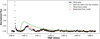 |
Fig. 2 Part of the TESS light curve from sector 6 corrected to the variability caused by stellar spots. The red curve and red interval mark the modulated flare model and the fit error, respectively. The green curve shows the recreated course of the stellar flare without the effects of foreshortening or stellar rotation. The gray points mark the data not used in the analysis. The translucent red area presents the uncertainty area. |
7 Discussion
We analyzed the starspot distribution on the star CD-36 3202. We also estimated its inclination angle, finding 70° ± 8°, and modeled its light curve in order to obtain the rotationally modulated LDE and estimate its parameters. It was possible to reconstruct a three-spot model with a mean spot temperature of approximately 4000 ± 765 K and an average total starspot area of about 11.61 ± 0.13% in sector 6 of TESS observations. The LDE lasted approximately 27 h, had a radius of about 3.°14, had an energy of about (3.99 ± 1.22) × 1035 erg, and occurred at  . For the first time, we were able to estimate the exact location of the flare in relation to the positions and sizes of the spots. The flaring region in the vicinity of the spot is about 12° from the center of spot number 3 (see Fig. 3). The white-light flare that occurred near the active region with the spots exhibited a very solar-like behavior, which is well documented in many images of the Sun from SDO/HMI (Namekata et al. 2017). The dependency between the occurrence of flares and starspots on K stars has received little attention in the literature. Roettenbacher & Vida (2018) showed that flares on K and M stars with amplitudes of less than 5% may be correlated with the groups of spots that create the minima in the light curve. However, other authors show that for the M stars, this correlation may not occur (Bicz et al. 2022; Feinstein et al. 2020; Ilin & Poppenhaeger 2022). Based on the analyzed event, we can confirm that flares may appear near starspots or active regions on K-type stars and we suggest that this type of star (partially convective flaring stars) should be the target of further observations (e.g., for the TESS mission) in order to analyze this relationship in more detail.
Our findings as to the flare’s location, estimated to  , are similar to the results of other authors. Ilin et al. (2021) analyzed four flares modulated by stellar rotation on four late-type M stars. These authors showed that the flares on fast-rotating (rotational periods from 2.7 h up to 8.4 h) M stars tend to appear at significantly higher latitudes compared with the Sun. On the Sun, flares occur in a belt around the equator up to the 30°. The flares found by Ilin et al. (2021) were located on significantly higher latitudes, above 55°. The flare analyzed in the present study, which is also above 30°, demonstrates that such phenomena are not only present in fully convective stars but also in partially convective stars. This suggests there may be similarities between the magnetic dynamo of young, rapidly rotating stars with different internal structures. The optical flux from the analyzed flare emitted towards hypothetical planets orbiting this star (or a similar star), assuming spin-orbit alignment of the planets, decreases by 29° ± 12°. This value is a relatively good fit to the relation found by Ilin et al. (2021) of relative optical flare energy emitted towards the planet in a star–planet system with a spin–orbit aligned for a typical superflare. It is worth noting that our findings refer only to the white-light emission. Stellar coronae are optically thin, and so the X-ray photons originating from flares may not be affected by the foreshortening effects similar to the effect that impacts the optical emission near the stellar limb. The X-ray flux received by the planets may therefore be much less attenuated.
The gray data points visible in Fig. 2 (around 1487.1 days) that were excluded from the fitting process indicate a decrease in the signal during the flare. This decrease is later repeated in the corresponding parts of the modulated flare (times about 1487.31 days and 1487.52 days). It can be seen that the moments of the beginning of the dimmings are separated in time by about 0.21 days and become shorter over time (107 min gray points, 30 min second dimming, 20 min third dimming). This could be caused by an optically thick absorption structure, such as a filament or a relatively cool loop, that partially or completely covers the flaring region. The loops above the flaring region slowly change their visible structure due to the evolution of the temperature and density of the loops (Heinzel & Shibata 2018; Song et al. 2016; Aschwanden 2005). The areas covered by flare–loop arcades are large and comparable to the size of active regions, which is well documented in many images of the Sun from SDO/AIA. In the case of stellar flares, the loop arcades can be even more extended. Another explanation could be the destabilization of the structure above the flaring region due to the flare and the eruption as a slow CME. Due to the motion of the CME, the smaller part of the flaring region is covered. For a simple estimation of the plasma parameters of the covering structure, we employed the cloud model (Heinzel & Shibata 2018). We hypothesized that the observed decrease (about 45% of the emission of the flaring region) is caused by the absorbing structure above the flaring region. The decrease occurred near the peak of the flare emission in the TESS bandpass, and so we assume that the temperature of the flaring region (e.g., flaring ribbons) during this period was 12 000 K. Additionally, we posit that the temperature of the overlying cloud is around 8000 K (e.g., Jejčič et al. 2018) in order to achieve a reasonable temperature for the cooler structure. The flaring region has a radius of about 3.°14 deg, which corresponds to a size of ~30 500 km on the star. We approximate the cloud as an arcade of the post-flare loops, which are semi-circular in shape and have a radius of 30 500 km. Using the radius of the flare loop and using the data on flare loops from Warmuth & Mann (2013), we estimate the loop cross-section radius as being equal to approximately 2800 km. Based on these parameters from a single loop, we estimate that approximately 11 loops would be required to completely cover the region below them. We tried to fit the absorption dip by varying the loop electron density using the covering structure, with an assumed temperature of 8000 K and a thickness of 5600 km. The resulting density we obtain is 7 × 1013 cm−3. The entire absorbing structure boasts a volume of roughly 3 × 1028 cm3. A high electron density in the range of ne ≥ 1012–1013 cm−3 is both unquestionably necessary and anticipated, primarily due to the intense evaporative processes occurring during super-flares (see discussion in Heinzel & Shibata 2018). While such high coronal densities have indeed been reported for some solar flares (Hiei 1982; Jejčič et al. 2018), the complexity of this issue combined with the numerous degrees of freedom necessitate further research in order to thoroughly investigate the proposed hypotheses.
Before the modulated flare, there was another flare at the TBJD of about 1486.85 days. This flare’s energy was (5.31 ± 2.03) × 1034 erg. We tried to also fit this event as a part of the modulated flare, but were unable to because the time interval between the corresponding parts of the modulations (e.g., local minima or local maxima) in the modulated flare should be separated in time by the rotational period of the star. Including this flare led to a 53 min time bias to the result, making it impossible to perform the fit correctly. This suggests that this flare was not part of the main event. The flare could be a precursor flare that led to destabilization of a great magnetic structure on the star and caused massive, long-lasting magnetic reconnection that led to an approximately 27 h stellar flare. Another explanation is that this flare is just a random flare that was not connected in any way to the mentioned LDE.
We compared the profile of the flare with the mean profile of the flare presented by Davenport et al. (2014) and with the mean profiles presented by Pietras et al. (2022; see Fig. 4). To include both the impulsive rise and the slow exponent decay, we used the time metric presented by Kowalski et al. (2013). We measured the light curve full-time width at half the maximum flux, denoted t1/2. The flare profile obtained during our analysis even though it has a faster rise time and slightly slower decay time, fits very well with the averaged one-component profile obtained by Pietras et al. (2022; see Fig. 4). Even though the duration time of this flare (approximately 27 h) is longer than any flare event ever observed on any star in TESS data (Pietras et al. 2022; Günther et al. 2020; Yang et al. 2023), it is very similar in appearance to the averaged profile (made from profiles of about 94 000 flares). This may suggest that the mechanism of the flares – magnetic reconnection – is a mechanism that gives similar events but with the energy released on different timescales.
Also, we compared the bolometric energy of the analyzed flare and its duration with the corresponding parameters of over 14 0000 flares detected on more than 25 000 stars (Pietras et al. 2022). The energies of the flare, both before and after correction for rotational modulation effects, fall within the scatter range of all the flares (see Fig. 5). Additionally, the parameters of the corrected flare (the green star in Fig. 5) position it noticeably closer to the exponential fit observed for all flares (the red line in Fig. 5). Similarly, the energy of the flare and the starspot area where the flare occurred (3.93 ± 0.3% of the stellar surface) fit very well to the flare energy–spot group area relation for superflares on solar-type stars presented by Maehara et al. (2015). These findings suggest that the energy-release mechanism for this particular flare may align with the typical process seen in white-light flares – heating caused by nonthermal electrons accelerated through magnetic reconnection (Brown 1971; Emslie 1978) – but that the energy is released on a much longer timescale than most of the observed stellar and solar flares (Pietras et al. 2022; Günther et al. 2020).
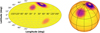 |
Fig. 3 Distribution of starspots on the star CD-36 3202 in sector 6 during the LDE flare. The bright region at a latitude of approximately 70° and longitude of approximately 100° is the flare from Fig. 2. The left panel presents the star in the Aitoff projection and the right panel presents the model of the star in the orthographic projection. |
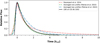 |
Fig. 4 Comparision of averaged flare profiles from Davenport et al. (2014) and Pietras et al. (2022) with the profile of the long-duration event analyzed here. The red curve presents the average flare profile presented by Davenport et al. (2014). The blue and green curves present the average flare profiles presented by Pietras et al. (2022). The green curve corresponds to the one fitted profile and the blue curve is a combination of two profiles. The black dashed curve corresponds to the analyzed modulated flare. |
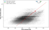 |
Fig. 5 Observed relations between flare energy and duration time. All of the flares detected in the TESS data by Pietras et al. (2022) are marked with black dots. The discrete flare duration bins result from the time resolution of the observations, which is equal to 2 min. The red triangles show the location of the centers of mass and the red dashed line presents the power-law fit. The centers of mass are the median duration time and median energy of the flares divided into 15 parts. The blue star and the green star show the energy of the analyzed flare before and after correction for rotational modulation, respectively. The black arrow presents the shift in energy between the modulated and demodulated flare. |
Acknowledgements
This work was partially supported by the program “Excel– lence Initiative – Research University” for years 2020–2026 for the University of Wrocław, project no. BPIDUB.4610.96.2021.KG. The computations were performed using resources provided by Wrocław Networking and Supercomputing Centre (https://wcss.pl/), computational grant number 569. We extend our gratitude to Professor Petr Heinzel for the invaluable discussions regarding the role of flare loops in the white light emission of stellar flares and for his help with cloud-model computations. The authors are grateful to the anonymous referee for constructive comments and suggestions, which have proved to be very helpful in improving the manuscript. This paper includes data collected by the TESS mission. Funding for the TESS mission is provided by NASA’s Science Mission Directorate.
Appendix A Estimation of the inclination angle of CD-36 3202
We used the stellar rotation period, P*, and radius, R*, in conjunction with the projection of rotational velocity υ sin(i), to deduce the stellar inclination angle, i. To address the statistical correlation between equatorial velocity and υ sin(i), we employed our newly developed tool, findinc_mc4. This software employs Equation A.1 and Monte-Carlo techniques to generate a probability density posterior for the inclination angle based on the provided measurements.
 (A.1)
(A.1)
We imposed the condition 0 < sin(i) < 1 while assuming Gaussian priors for υ sin(i), P*, and R*. The inclination posteriors exhibit non-Gaussian behavior across various stars, although they can be approximated by a double-Gaussian fit. The inclination value corresponds to the angle that maximizes the distribution. For uncertainty estimation, we calculate the standard deviation of the posterior distribution. Using the findinc_mc software, we evaluated the inclination of the star as equal to 70° ± 8° (see Figure A.1). During the calculation process, we used the estimated rotational period, which is equal to P* = 0.23536 ± 0.00046 day, and we assumed the projection of rotation velocity vsin(i) = 170 ± 17 km/s (Torres et al. 2006). The radius of the star R* was taken from the MAST catalog.
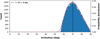 |
Fig. A.1 Posterior distribution of stellar inclination angles (blue histogram), the smoothed probability density posterior (red curve), and the maximum of the posterior (black dotted line). |
References
- Aschwanden, M. J. 2005, Physics of the Solar Corona. An Introduction with Problems and Solutions, 2nd edn (Praxis Publishing Ltd.) [Google Scholar]
- Bell, C. P. M., Mamajek, E. E., & Naylor, T. 2015, MNRAS, 454, 593 [Google Scholar]
- Bicz, K., Falewicz, R., Pietras, M., Siarkowski, M., & Pres, P. 2022, ApJ, 935, 102 [NASA ADS] [CrossRef] [Google Scholar]
- Biermann, L. 1941, Vierteljahressch. Astron. Gesellsch., 76, 194 [NASA ADS] [Google Scholar]
- Bogner, M., Stelzer, B., & Raetz, S. 2022, Astron. Nachr., 343, e210079 [CrossRef] [Google Scholar]
- Bray, R. J., & Loughhead, R. E. 1964, Sunspots (London: Chapman & Hall) [Google Scholar]
- Brown, J. C. 1971, Sol. Phys., 18, 489 [Google Scholar]
- Chitre, S. M. 1963, MNRAS, 126, 431 [NASA ADS] [Google Scholar]
- Claret, A. 2017, A&A, 600, A30 [NASA ADS] [CrossRef] [EDP Sciences] [Google Scholar]
- Davenport, J. R. A., Hawley, S. L., Hebb, L., et al. 2014, ApJ, 797, 122 [Google Scholar]
- Davenport, J. R. A., Covey, K. R., Clarke, R. W., et al. 2019, ApJ, 871, 241 [Google Scholar]
- Deinzer, W. 1965, ApJ, 141, 548 [NASA ADS] [CrossRef] [Google Scholar]
- Dicke, R. H. 1970, ApJ, 159, 25 [NASA ADS] [CrossRef] [Google Scholar]
- Emslie, A. G. 1978, ApJ, 224, 241 [NASA ADS] [CrossRef] [Google Scholar]
- Feinstein, A. D., Montet, B. T., Ansdell, M., et al. 2020, AJ, 160, 219 [Google Scholar]
- Feoktistov, V., & Janaqi, S. 2004, Proceedings of the 18th International Parallel and Distributed Processing Symposium (IPDPS’04), 165 [CrossRef] [Google Scholar]
- Fletcher, R. 1987, Practical Methods of Optimization, 2nd edn. (New York, NY, USA: John Wiley & Sons) [Google Scholar]
- Flores, C., Connelley, M. S., Reipurth, B., & Duchêne, G. 2022, ApJ, 925, 21 [NASA ADS] [CrossRef] [Google Scholar]
- Foreman-Mackey, D., Luger, R., Czekala, I., et al. 2021, https://doi.org/10.5281/zenodo.1998447 [Google Scholar]
- Gryciuk, M., Siarkowski, M., Sylwester, J., et al. 2017, Sol. Phys., 292, 77 [NASA ADS] [CrossRef] [Google Scholar]
- Günther, M. N., Zhan, Z., Seager, S., et al. 2020, AJ, 159, 60 [Google Scholar]
- Heinzel, P., & Shibata, K. 2018, ApJ, 859, 143 [NASA ADS] [CrossRef] [Google Scholar]
- Hiei, E. 1982, Sol. Phys., 80, 113 [NASA ADS] [CrossRef] [Google Scholar]
- Howard, W. S., Corbett, H., Law, N. M., et al. 2019, ApJ, 881, 9 [NASA ADS] [CrossRef] [Google Scholar]
- Howard, W. S., Corbett, H., Law, N. M., et al. 2020, ApJ, 902, 115 [Google Scholar]
- Hoyle, F. 1949, Some recent researches in solar physics (London-New-York: Cambridge Univ. Press) [Google Scholar]
- Ilin, E., & Poppenhaeger, K. 2022, MNRAS, 513, 4579 [NASA ADS] [CrossRef] [Google Scholar]
- Ilin, E., Poppenhaeger, K., Schmidt, S. J., et al. 2021, MNRAS, 507, 1723 [CrossRef] [Google Scholar]
- Jejčič, S., Kleint, L., & Heinzel, P. 2018, ApJ, 867, 134 [NASA ADS] [CrossRef] [Google Scholar]
- Kovári, Z., Vilardell, F., Ribas, I., et al. 2007, Astron. Nachr., 328, 904 [CrossRef] [Google Scholar]
- Kowalski, A. F., Hawley, S. L., Wisniewski, J. P., et al. 2013, ApJS, 207, 15 [NASA ADS] [CrossRef] [Google Scholar]
- Kowalski, A. F., Hawley, S. L., Carlsson, M., et al. 2015, Sol. Phys., 290, 3487 [NASA ADS] [CrossRef] [Google Scholar]
- Luger, R., Agol, E., Foreman-Mackey, D., et al. 2019, AJ, 157, 64 [Google Scholar]
- Maehara, H., Shibayama, T., Notsu, Y., et al. 2015, Earth Planets Space, 67, 59 [NASA ADS] [CrossRef] [Google Scholar]
- Mathur, S., García, R. A., Ballot, J., et al. 2014, A&A, 562, A124 [NASA ADS] [CrossRef] [EDP Sciences] [Google Scholar]
- Namekata, K., Sakaue, T., Watanabe, K., et al. 2017, ApJ, 851, 91 [Google Scholar]
- Pietras, M., Falewicz, R., Siarkowski, M., Bicz, K., & Pres, P. 2022, ApJ, 935, 143 [NASA ADS] [CrossRef] [Google Scholar]
- Ricker, G. R., Winn, J. N., Vanderspek, R., et al. 2014, Space Telescopes and Instrumentation 2014: Optical, Infrared, and Millimeter Wave, 9143, 914320 [Google Scholar]
- Roettenbacher, R. M., & Vida, K. 2018, ApJ, 868, 3 [NASA ADS] [CrossRef] [Google Scholar]
- Salvatier, J., Wiecki, T. V., & Fonnesbeck, C. 2016, PeerJ Comput. Sci., 2, e55 [Google Scholar]
- Shibayama, T., Maehara, H., Notsu, S., et al. 2013, ApJS, 209, 5 [Google Scholar]
- Song, Q., Wang, J.-S., Feng, X., & Zhang, X. 2016, ApJ, 821, 83 [NASA ADS] [CrossRef] [Google Scholar]
- Theano Development Team (Al-Rfou, R., et al.) 2016, arXiv e-prints [arXiv:arXiv:1605.02688] [Google Scholar]
- Torres, C. A. O., Quast, G. R., da Silva, L., et al. 2006, A&A, 460, 695 [NASA ADS] [CrossRef] [EDP Sciences] [Google Scholar]
- Warmuth, A., & Mann, G. 2013, A&A, 552, A87 [NASA ADS] [CrossRef] [EDP Sciences] [Google Scholar]
- Yang, H., Liu, J., Gao, Q., et al. 2017, ApJ, 849, 36 [NASA ADS] [CrossRef] [Google Scholar]
- Yang, Z., Zhang, L., Meng, G., et al. 2023, A&A, 669, A15 [NASA ADS] [CrossRef] [EDP Sciences] [Google Scholar]
All Tables
All Figures
|
Fig. 1 TESS light curves from sectors 6 and 7, with a reconstructed starspot model and the unspotted stellar level highlighted. Left side: Part of the TESS light curve from sector 6 (black dots) during which the long-duration flare occurred, with the starspot model that recreates the curve (red line). The green, blue, and orange curves present the contribution of individual spots to the whole light curve. Right side: Part of the TESS light curve from sector 7 (black dots) with the estimated unspotted level of the star marked with a purple line. |
| In the text | |
|
Fig. 2 Part of the TESS light curve from sector 6 corrected to the variability caused by stellar spots. The red curve and red interval mark the modulated flare model and the fit error, respectively. The green curve shows the recreated course of the stellar flare without the effects of foreshortening or stellar rotation. The gray points mark the data not used in the analysis. The translucent red area presents the uncertainty area. |
| In the text | |
|
Fig. 3 Distribution of starspots on the star CD-36 3202 in sector 6 during the LDE flare. The bright region at a latitude of approximately 70° and longitude of approximately 100° is the flare from Fig. 2. The left panel presents the star in the Aitoff projection and the right panel presents the model of the star in the orthographic projection. |
| In the text | |
|
Fig. 4 Comparision of averaged flare profiles from Davenport et al. (2014) and Pietras et al. (2022) with the profile of the long-duration event analyzed here. The red curve presents the average flare profile presented by Davenport et al. (2014). The blue and green curves present the average flare profiles presented by Pietras et al. (2022). The green curve corresponds to the one fitted profile and the blue curve is a combination of two profiles. The black dashed curve corresponds to the analyzed modulated flare. |
| In the text | |
|
Fig. 5 Observed relations between flare energy and duration time. All of the flares detected in the TESS data by Pietras et al. (2022) are marked with black dots. The discrete flare duration bins result from the time resolution of the observations, which is equal to 2 min. The red triangles show the location of the centers of mass and the red dashed line presents the power-law fit. The centers of mass are the median duration time and median energy of the flares divided into 15 parts. The blue star and the green star show the energy of the analyzed flare before and after correction for rotational modulation, respectively. The black arrow presents the shift in energy between the modulated and demodulated flare. |
| In the text | |
|
Fig. A.1 Posterior distribution of stellar inclination angles (blue histogram), the smoothed probability density posterior (red curve), and the maximum of the posterior (black dotted line). |
| In the text | |
Current usage metrics show cumulative count of Article Views (full-text article views including HTML views, PDF and ePub downloads, according to the available data) and Abstracts Views on Vision4Press platform.
Data correspond to usage on the plateform after 2015. The current usage metrics is available 48-96 hours after online publication and is updated daily on week days.
Initial download of the metrics may take a while.