| Issue |
A&A
Volume 677, September 2023
|
|
|---|---|---|
| Article Number | L12 | |
| Number of page(s) | 4 | |
| Section | Letters to the Editor | |
| DOI | https://doi.org/10.1051/0004-6361/202347704 | |
| Published online | 12 September 2023 | |
Letter to the Editor
Stellar obliquity and planetary albedo in HAT-P-32
Derived from the TESS light curve
1
Thüringer Landessternwarte Tautenburg, Sternwarte 5, 07778 Tautenburg, Germany
e-mail: This email address is being protected from spambots. You need JavaScript enabled to view it.
2
Hamburger Sternwarte, Universität Hamburg, Gojenbergsweg 112, 21029 Hamburg, Germany
Received:
11
August
2023
Accepted:
28
August
2023
Abstract
HAT-P-32 is an exceptional planetary system. Its active F-type host star is orbited by a hot Jupiter, the evaporation of which produces a giant structure of tidal tails. We analyze the light curve of HAT-P-32 obtained by the Transiting Exoplanet Survey Satellite (TESS) and find a secondary eclipse superimposed on photometric modulation likely caused by stellar rotation. We estimate a secondary eclipse depth of (1.4 ± 0.4)×10−4. Adopting a prior of 1962 ± 83 K for the effective planetary dayside temperature yields values of 0.16 ± 0.07 for the geometric albedo and an associated estimate of 0.46 ± 0.21 for the circulation efficiency of HAT-P-32 b, which favor a dark and windy scenario for the atmosphere. Our analysis of the photometric modulation yields a stellar rotation period of 2.974 ± 0.004 d, implying a value of 79° for the inclination of the stellar rotation axis with a 95% credible interval from 70° to 88°. This constraint further allows us to estimate a value of (84.9 ± 1.5)° for the three-dimensional obliquity. Despite showing an almost polar planetary orbit, the host star is, therefore, seen nearly equator on.
Key words: planets and satellites: atmospheres / techniques: photometric / planets and satellites: individual: HAT-P-32
© The Authors 2023
 Open Access article, published by EDP Sciences, under the terms of the Creative Commons Attribution License (https://creativecommons.org/licenses/by/4.0), which permits unrestricted use, distribution, and reproduction in any medium, provided the original work is properly cited.
This article is published in open access under the Subscribe to Open model. This email address is being protected from spambots. You need JavaScript enabled to view it. to support open access publication.
1. Introduction
The hot Jupiter HAT-P-32 b revolves around an active late F-type star (Hartman et al. 2011) in a circular and almost polar orbit (Albrecht et al. 2012; Zhao et al. 2014). Recently, high-resolution transmission spectroscopy of the He Iλ10833 triplet lines in the HAT-P-32 system revealed an enormous structure of material evaporated from the planet, which forms two giant tails trailing and preceding the planet on its orbit (Czesla et al. 2022; Zhang et al. 2023). While transmission spectroscopy is sensitive to the terminator and upper atmosphere of the planet, its dayside is better studied by photometric phase curves and secondary eclipses (e.g., Parmentier & Crossfield 2018).
Observations of the secondary eclipse of HAT-P-32 b in the infrared regime have allowed us to constrain the dayside temperature of HAT-P-32 b. Zhao et al. (2014) analyzed ground-based H- and Ks-band photometry as well as light curves obtained with the Spitzer Space Telescope’s Infrared Array Camera (IRAC) at 3.6 and 4.5 μm and found the planetary spectrum to be well described by a blackbody with a temperature of 2042 ± 50 K. Nikolov et al. (2018) present secondary eclipse measurements in the 1.123–1.644 μm range obtained with the Wide Field Camera 3 on board the Hubble Space Telescope. Combined with the data presented by Zhao et al. (2014), the authors report that the spectrum of HAT-P-32 b is best described by a blackbody with a temperature of 1995 ± 17 K. A comparable dayside temperature of 1962 ± 83 K was determined in the retrieval analysis by Changeat et al. (2022), who present no new eclipse data, however. In their analysis of z′-band eclipse photometry (≈900 ± 60 nm, Fukugita et al. 1996), Mallonn et al. (2019) derived an upper limit of 0.2 for the geometric albedo of HAT-P-32 b.
We here examine the Transiting Exoplanet Survey Satellite (TESS) light curve, which covers the optical to near-infrared band from about 400 nm to 1000 nm, to search for stellar rotational modulation and the secondary planetary eclipse. The TESS light curve of HAT-P-32 was previously presented by Maciejewski et al. (2023), who unsuccessfully searched for transits of additional planets in the system.
2. Observations
TESS observed HAT-P-32 from 29 October to 26 November 2022 (TESS input catalog number 292152376) with 20 s cadence. We downloaded the data from the MAST1 archive. Our analysis is based on the simple aperture photometry (SAP_FLUX) and its error (SAP_FLUX_ERROR). Additionally, we restricted our analysis to good quality data points (QUALITY=0). Using the βσ method (Czesla et al. 2018), we estimated a signal-to-noise ratio (S/N) of 280 per bin for the scatter in the light curve, which is only slightly lower than the median S/N of 295 derived using the pipeline-produced uncertainty of the flux. The latter, therefore, contains all relevant noise sources, and we use it in our analysis.
In Fig. 1, we show the light curve without the primary transits. The light curve shows three gaps with a length of about 0.2 d, illustrating that there is a natural subdivision into four sections with an approximately equal duration of about 7 d. The separations are made at JDT = 2889.5, 2896.2, and 2903.5 (JDT denotes BJDTDB − 2457000). In the top panel of Fig. 1, we show the sections normalized by their respective median. To improve the normalization, we fit the individual sections of the light curve using linear models. Division by the best fit yields the normalized light curve shown in the bottom panel of Fig. 1, which is the basis for our analysis.
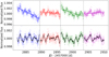 |
Fig. 1. TESS light curve of HAT-P-32. Top: median-normalized TESS light curve of HAT-P-32 without primary transits binned at 14 min cadence. Solid lines indicate best-fit linear models. Bottom: light curve normalized by linear models along with smoothed curve (solid black). In both panels, the colors of the data# points indicate the individual sections and the vertical lines highlight the separations between the sections. |
3. Period analysis
The light curve in Fig. 1 clearly shows modulation with a seemingly periodic behavior. To substantiate that impression, we first computed the generalized Lomb-Scargle (GLS) periodogram (Ferraz-Mello 1981; Zechmeister & Kürster 2009) of the entire light curve (Fig. 2, blue), which shows a prominent peak at 1.487 ± 0.002 d; we call this the 1.5 d period for the sake of the discussion. The semi-amplitude of the best-fit sine curve corresponding to the 1.5 d period is (4.7 ± 0.2)×10−4.
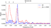 |
Fig. 2. Generalized Lomb-Scargle periodogram for the entire TESS light curve of HAT-P-32 (blue) and the later part (JDT > 2900), red). |
To check the persistence of the 1.5 d period, we performed a sliding window analysis. To that end, we defined a 4 d long window, shifted it across the light curve by increments of 2 d, and computed the GLS periodogram of the data in the window. The resulting period evolution of the dominant peak is plotted in Fig. 3. Clearly, the 1.5 d period prevails until about JDT 2900, after which the best-fit period increases to values in the range of two to four days.
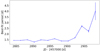 |
Fig. 3. Period of the dominant peak obtained by the shifting window GLS analysis. |
A plausible explanation for the observed variability in a fast-rotating, active star such as HAT-P-32 is rotational modulation caused by starspots. In this case, 1.5 d becomes a candidate for the stellar rotation period. However, it is not uncommon in such analyses to find twice the actual rotation period to produce the dominant signal, because any starspot is only visible for half a rotation unless it is located close enough to the pole to remain permanently visible due to the inclination of the stellar rotation axis. Therefore, we consider 2.974 d another likely candidate for the actual stellar rotation period, the 3 d period for short.
To examine the plausibility of the hypothesis that the 3 d period is the stellar rotation period, we had a closer look at the results from our sliding window analysis. This shows that both the 1.5 d and the 3 d period are present at various levels throughout the dataset with the 1.5 d period dominating until JDT = 2900. After this, its power dramatically drops off and it is overtaken by that of the 3 d period. In Fig. 2, we also show the periodogram obtained using only the data after JDT = 2900, which, indeed, has its most significant peak at 3 d with a secondary peak at 1.5 d remaining.
As an alternative to the GLS periodogram, we applied the non-parametric string length method (Dworetsky 1983). Here, the data are folded with various trial periods and the length of the line connecting the phase-ordered set of data points is calculated. This so-called string length is shorter if the folding is done with periods representing the periodicity in the data well. In Fig. 4, we show the string length of the light curve of HAT-P-32 for a set of trial periods between one and four days before and after JDT 2900. In the earlier part of the light curve, a 1.5 d and a 3 d signal are apparent, which can both be caused by a 1.5 d periodicity. In the later part, however, only a 3 d signal is present, albeit very broad.
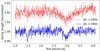 |
Fig. 4. String length as a function of trial period before and after JDT 2902. |
Both the periodogram and string length results are consistent with the 1.5 d signal being the harmonic of a true 3 d stellar rotation period. Neither the periodogram nor the string length allow us to determine the period of the 3 d signal directly with great precision. We attribute this to the rather short duration of the part of the light curve where it dominates and its transitional nature. A plausible scenario for the observed behavior is that in the early TESS sectors two surface spots separated by ≈180° in longitude produced the 1.5 d harmonic signal. With time, this spot configuration evolved into one dominant spot showing the rotational 3 d period. Nonetheless, the well-determined period of the harmonic is better suited to fix the stellar rotation period.
HAT-P-32 has a stellar companion of M1.5V type at a separation of 2.9″ (Zhao et al. 2014). Given the TESS pixel scale of 21″, the light of this secondary certainly contaminates the light curve of HAT-P-32. Zhao et al. (2014) list flux ratios for the primary F-type and secondary M-type component in the system for various photometric bands, which allow us to estimate the magnitude of the contamination. Adopting the i′-band flux ratio of 0.006 ± 0.002 as an approximation to the ratio observed by TESS makes the primary brighter by a factor of 166 ± 55, and bluer bands yield even larger contrasts. To be responsible for the observed photometric variation with an amplitude on the order of 5 × 10⁻⁴, the companion would have to show photometric variation with a semi-amplitude of about 8%. While such large photometric variations in an M1.5V star may not be entirely excluded, they would be exceptional (Santos et al. 2019) and the explanation unnecessarily complicated (Sect. 5).
4. The secondary eclipse observed by TESS
While the extraction of the entire smooth phase curve of HAT-P-32 b from the rotational modulation in the TESS light curve seems very challenging, a search for the secondary eclipse, which is expected to produce a well-defined dip with a known position and duration, is more promising. To study the eclipse, we first extracted a total of 12 sections of the light curve centered on orbital phase 0.5, where the eclipse is expected. We specifically used sections ranging from orbital phase 0.167–0.833, which covers 11 transit durations or 1.43 d and at least 4000 out-of-eclipse data points. We then fit a polynomial model to the out-of-eclipse data of the individual sections, divided by the best-fit model, and combined the thus normalized eclipse sections. A binned version of the combined, phase-folded light curve using a third-order polynomial for normalization is shown in Fig. 5. Polynomial orders smaller than three leave strong systematic variation in the light curve, but the result does not critically depend on the normalizing polynomial of up to order six. Based on the light curve shown in Fig. 5, we calculated a mean out-of-eclipse level, μout, of 1.000000 ± 0.000014 and a corresponding in-eclipse level, μin, of 0.99986 ± 0.00004. The resulting eclipse depth, therefore, becomes δm = μout − μin = (1.4 ± 0.4)×10−4.
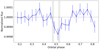 |
Fig. 5. Phase-folded, binned, and normalized eclipse light curve. |
The total eclipse depth is the sum of thermal and reflective scattering contributions so that δtot = δth + δrefl. The reflective contribution to the eclipse depth, δrefl, and the geometric albedo, Ag, are related by (e.g., López-Morales & Seager 2007)
 (1)
(1)
where Rp is the planetary radius and a denotes the semi-major axis. The thermal contribution to the eclipse depth, δth, is determined by the ratio of the stellar and planetary thermal fluxes in the TESS bandpass. Adopting the parametrization of Cowan & Agol (2011), the dayside effective temperature of the planet can be obtained by
![Mathematical equation: $$ \begin{aligned} T_{\rm d} = T_{\star } \sqrt{\frac{R_{\star }}{a}} \left[\left(\frac{2}{3} - \frac{5}{12}\epsilon \right) (1-A_{\rm B}) \right]^{\frac{1}{4}} ,\end{aligned} $$](/articles/aa/full_html/2023/09/aa47704-23/aa47704-23-eq2.gif) (2)
(2)
where T⋆ and R⋆ are the stellar effective temperature and radius, ϵ represents the circulation efficiency, and AB is the Bond albedo (López-Morales & Seager 2007).
Assuming blackbody spectra for the star and planet as well as Lambertian spherical surfaces, which yields  (e.g., Lester et al. 1979), one is left with a problem with two free parameters, namely ϵ and Ag or, alternatively, Td and Ag. Using the temperature estimates of 1962 ± 83 K from Changeat et al. (2022) and 2042 ± 50 K from Nikolov et al. (2018) as a prior on the dayside temperature yields estimates of 0.16 ± 0.07 and 0.14 ± 0.06 for the geometric planetary albedo, assuming a uniform prior density on this parameter. The associated values for the circulation efficiency, obtained by Eq. (2), are 0.46 ± 0.21 and 0.33 ± 0.18.
5. Discussion and conclusion
We analyzed the TESS light curve of the HAT-P-32 system and found periodic variation, which is most consistent with stellar rotational modulation with a rotation period of 2.974 ± 0.004 d (Sect. 3), although our periodogram analysis is mostly sensitive to the first harmonic of this period. The effective temperature of HAT-P-32 implies a spectral type of F7 for HAT-P-32. The star is highly active as shown by its X-ray luminosity of 2.3 × 1029 erg s−1 (Czesla et al. 2022), which is consistent with that of other F-type stars with similar rotation periods (Pizzocaro et al. 2019). Its observed projected rotational velocity is entirely compatible with the mean value for F7 V stars of v sin i = 25 km s−1 (Fukuda 1982). Given the rotation period and the radius of the star (Table 1), an estimate of 20.73 ± 0.27 km s−1 was derived for the stellar equatorial rotation speed, implying a high value for the inclination of the stellar rotation axis. By combining the rotation period with the stellar radius and projected rotation speed, we specifically derived a value of 79° with a 95% highest probability density credible interval ranging from 70° to 88°. Combining this constraint with the sky-projected obliquity and orbital inclination (Table 1), also allowed us to estimate a value of (84.9 ± 1.5)° for the obliquity, Ψ, that is, the angle between the planetary orbit normal and the stellar rotation axis. This value fits in with an alleged preponderance of polar orbits in misaligned systems (Albrecht et al. 2021; Attia et al. 2023), the physical reality of which remains, however, controversial (Dong & Foreman-Mackey 2023; Siegel et al. 2023). Our results provide no indication for significant contamination by the M1.5V-type companion (Sect. 3). Despite the large obliquity of the planetary orbit, the star is seen almost equator-on, adding another peculiarity to this outstanding planetary system.
Relevant system parameters of HAT-P-32.
We measured the secondary eclipse depth from the TESS light curve and modeled the result taking into account reflective and thermal contributions to the planetary flux and assuming blackbody spectra. Although the TESS band is relatively broad, covering wavelengths from about 400 nm to 1000 nm, it provides some leverage on the reflective component of the secondary eclipse depth and, thus, albedo, which is more prominent in the optical than the infrared range. Varying the planetary dayside temperature within the range of published values derived from infrared eclipse photometry yields a low geometric albedo, consistent with the previously reported upper limit of 0.2 in the z′ band (Mallonn et al. 2019). Low albedos require relatively higher circulation efficiencies. In fact, low geometric albedos at the wavelength range covered by TESS are not uncommon for hot Jupiters such as HAT-P-32 b as demonstrated by the sample presented in Table 2, which was selected to span a cross section of equilibrium temperatures and, thus, irradiation conditions; additionally, we refer to the larger sample studies by Schwartz & Cowan (2015) and Wong et al. (2021). Our results also tend to support the atmospheric “dark and windy” scenario proposed by Nikolov et al. (2018), characterized by a low albedo and more efficient energy redistribution.
Geometric albedos for a sample of planets sorted by equilibrium temperature.
Barbara A. Mikulski Archive for Space Telescopes.
Acknowledgments
S.C. acknowledges the support of the DFG priority program SPP 1992 “Exploring the Diversity of Extrasolar Planets” (CZ 222/5-1). P.C.S. acknowledges support through DLR 50OR2205. This work made extensive use of the software packages PyAstronomy (Czesla et al. 2019), emcee (Foreman-Mackey et al. 2013), NumPy (Harris et al. 2020), and Matplotlib (Hunter 2007). Funding for the TESS mission is provided by NASA’s Science Mission directorate.
References
- Albrecht, S., Winn, J. N., Johnson, J. A., et al. 2012, ApJ, 757, 18 [NASA ADS] [CrossRef] [Google Scholar]
- Albrecht, S. H., Marcussen, M. L., Winn, J. N., Dawson, R. I., & Knudstrup, E. 2021, ApJ, 916, L1 [NASA ADS] [CrossRef] [Google Scholar]
- Attia, O., Bourrier, V., Delisle, J. B., & Eggenberger, P. 2023, A&A, 674, A120 [NASA ADS] [CrossRef] [EDP Sciences] [Google Scholar]
- Changeat, Q., Edwards, B., Al-Refaie, A. F., et al. 2022, ApJS, 260, 3 [NASA ADS] [CrossRef] [Google Scholar]
- Cowan, N. B., & Agol, E. 2011, ApJ, 729, 54 [Google Scholar]
- Czesla, S., Molle, T., & Schmitt, J. H. M. M. 2018, A&A, 609, A39 [NASA ADS] [CrossRef] [EDP Sciences] [Google Scholar]
- Czesla, S., Schröter, S., Schneider, C. P., et al. 2019, Astrophysics Source Code Library [record ascl:1906.010] [Google Scholar]
- Czesla, S., Lampón, M., Sanz-Forcada, J., et al. 2022, A&A, 657, A6 [NASA ADS] [CrossRef] [EDP Sciences] [Google Scholar]
- Dong, J., & Foreman-Mackey, D. 2023, AJ, 166, 112 [NASA ADS] [CrossRef] [Google Scholar]
- Dworetsky, M. M. 1983, MNRAS, 203, 917 [NASA ADS] [Google Scholar]
- Ferraz-Mello, S. 1981, AJ, 86, 619 [NASA ADS] [CrossRef] [Google Scholar]
- Foreman-Mackey, D., Hogg, D. W., Lang, D., & Goodman, J. 2013, PASP, 125, 306 [Google Scholar]
- Fukuda, I. 1982, PASP, 94, 271 [NASA ADS] [CrossRef] [Google Scholar]
- Fukugita, M., Ichikawa, T., Gunn, J. E., et al. 1996, AJ, 111, 1748 [Google Scholar]
- Harris, C. R., Millman, K. J., van der Walt, S. J., et al. 2020, Nature, 585, 357 [NASA ADS] [CrossRef] [Google Scholar]
- Hartman, J. D., Bakos, G. Á., Torres, G., et al. 2011, ApJ, 742, 59 [NASA ADS] [CrossRef] [Google Scholar]
- Hunter, J. D. 2007, Comput. Sci. Eng., 9, 90 [NASA ADS] [CrossRef] [Google Scholar]
- Jansen, T., & Kipping, D. 2020, MNRAS, 494, 4077 [Google Scholar]
- Lester, T. P., McCall, M. L., & Tatum, J. B. 1979, JRASC, 73, 233 [NASA ADS] [Google Scholar]
- López-Morales, M., & Seager, S. 2007, ApJ, 667, L191 [CrossRef] [Google Scholar]
- Maciejewski, G., Fernández, M., Sota, A., et al. 2023, Acta Astron., 73, 57 [NASA ADS] [Google Scholar]
- Mallonn, M., Köhler, J., Alexoudi, X., et al. 2019, A&A, 624, A62 [NASA ADS] [CrossRef] [EDP Sciences] [Google Scholar]
- Nikolov, N., Sing, D. K., Goyal, J., et al. 2018, MNRAS, 474, 1705 [NASA ADS] [CrossRef] [Google Scholar]
- Parmentier, V., & Crossfield, I. J. M. 2018, Handbook of Exoplanets (Springer International Publishing), 1419 [CrossRef] [Google Scholar]
- Pizzocaro, D., Stelzer, B., Poretti, E., et al. 2019, A&A, 628, A41 [NASA ADS] [CrossRef] [EDP Sciences] [Google Scholar]
- Santos, A. R. G., García, R. A., Mathur, S., et al. 2019, ApJS, 244, 21 [Google Scholar]
- Schwartz, J. C., & Cowan, N. B. 2015, MNRAS, 449, 4192 [NASA ADS] [CrossRef] [Google Scholar]
- Siegel, J. C., Winn, J. N., & Albrecht, S. H. 2023, ApJ, 950, L2 [NASA ADS] [CrossRef] [Google Scholar]
- Wang, Y.-H., Wang, S., Hinse, T. C., et al. 2019, AJ, 157, 82 [NASA ADS] [CrossRef] [Google Scholar]
- Wong, I., Benneke, B., Shporer, A., et al. 2020, AJ, 159, 104 [Google Scholar]
- Wong, I., Kitzmann, D., Shporer, A., et al. 2021, AJ, 162, 127 [NASA ADS] [CrossRef] [Google Scholar]
- Zechmeister, M., & Kürster, M. 2009, A&A, 496, 577 [CrossRef] [EDP Sciences] [Google Scholar]
- Zhang, Z., Morley, C. V., Gully-Santiago, M., et al. 2023, Sci. Adv., 9, eadf8736 [NASA ADS] [CrossRef] [Google Scholar]
- Zhao, M., O’Rourke, J. G., Wright, J. T., et al. 2014, ApJ, 796, 115 [NASA ADS] [CrossRef] [Google Scholar]
All Tables
All Figures
|
Fig. 1. TESS light curve of HAT-P-32. Top: median-normalized TESS light curve of HAT-P-32 without primary transits binned at 14 min cadence. Solid lines indicate best-fit linear models. Bottom: light curve normalized by linear models along with smoothed curve (solid black). In both panels, the colors of the data# points indicate the individual sections and the vertical lines highlight the separations between the sections. |
| In the text | |
|
Fig. 2. Generalized Lomb-Scargle periodogram for the entire TESS light curve of HAT-P-32 (blue) and the later part (JDT > 2900), red). |
| In the text | |
|
Fig. 3. Period of the dominant peak obtained by the shifting window GLS analysis. |
| In the text | |
|
Fig. 4. String length as a function of trial period before and after JDT 2902. |
| In the text | |
|
Fig. 5. Phase-folded, binned, and normalized eclipse light curve. |
| In the text | |
Current usage metrics show cumulative count of Article Views (full-text article views including HTML views, PDF and ePub downloads, according to the available data) and Abstracts Views on Vision4Press platform.
Data correspond to usage on the plateform after 2015. The current usage metrics is available 48-96 hours after online publication and is updated daily on week days.
Initial download of the metrics may take a while.