| Issue |
A&A
Volume 681, January 2024
|
|
|---|---|---|
| Article Number | A99 | |
| Number of page(s) | 14 | |
| Section | Stellar structure and evolution | |
| DOI | https://doi.org/10.1051/0004-6361/202347594 | |
| Published online | 23 January 2024 | |
Asteroseismic modelling strategies in the PLATO era
II. Automation of seismic inversions and quality assessment procedure
1
Observatoire de Genève, Université de Genève,
Chemin Pegasi 51,
1290
Versoix,
Switzerland
e-mail: jerome.betrisey@unige.ch
2
STAR Institute, University of Liège,
19C Allée du 6 Août,
4000
Liège,
Belgium
3
LESIA, Observatoire de Paris, Université PSL, CNRS, Sorbonne Université, Université Paris-Cité,
5 place Jules Janssen,
92195
Meudon,
France
Received:
28
July
2023
Accepted:
29
October
2023
Context. In the framework of the PLATO mission, to be launched in late 2026, seismic inversion techniques will play a key role in determining the mission precision requirements in terms of stellar mass, radius, and age. It is therefore relevant to discuss the challenges of the automation of seismic inversions, which were originally developed for individual modelling.
Aims. We tested the performance of our newly developed quality assessment procedure of seismic inversions, which was designed for pipeline implementation.
Methods. We applied our assessment procedure to a testing set composed of 26 reference models. We divided our testing set into two categories: calibrator targets whose inversion behaviour is well known from the literature and targets for which we assessed the quality of the inversion manually. We then compared the results of our assessment procedure with our expectations as a human modeller for three types of inversions: the mean density inversion, the acoustic radius inversion, and the central entropy inversion.
Results. We find that our quality assessment procedure performs as well as a human modeller. The mean density inversion and the acoustic radius inversion are suited to large-scale applications, but not the central entropy inversion, at least in its current form.
Conclusions. Our assessment procedure shows promising results for a pipeline implementation. It is based on the by-products of the inversion and therefore requires few numerical resources to quickly assess the quality of an inversion result.
Key words: stars: solar-type / asteroseismology / stars: fundamental parameters / stars: interiors
© The Authors 2024
 Open Access article, published by EDP Sciences, under the terms of the Creative Commons Attribution License (https://creativecommons.org/licenses/by/4.0), which permits unrestricted use, distribution, and reproduction in any medium, provided the original work is properly cited.
This article is published in open access under the Subscribe to Open model. Subscribe to A&A to support open access publication.
1 Introduction
Convective motions in the upper layers of solar-type stars generate a wide range of stellar oscillations. By studying these oscillations, asteroseismology enables us to probe the stellar interior and characterise the stellar parameters with a precision and accuracy that is difficult to match with other standard techniques for non-binary stars. Asteroseismology has undergone rapid development over the past two decades. The launch of space-based photometry missions such as CoRoT (Baglin et al. 2009), Kepler (Borucki et al. 2010), and TESS (Ricker et al. 2015) initiated the so-called photometry revolution. The unprecedented data quality from these missions allows us to use cutting edge techniques, the so-called seismic inversions (see e.g. Reese et al. 2012; Buldgen et al. 2015b,a, 2018; Bétrisey & Buldgen 2022), that were, until these missions, restricted to helioseismology (see e.g. Basu & Antia 2008; Kosovichev 2011; Buldgen et al. 2019c, 2022a; Christensen-Dalsgaard 2021, for reviews). Such seismic inversions were applied to various asteroseismic targets (see e.g. di Mauro 2004; Buldgen et al. 2016a, b, 2017a, 2019b,a, 2022b; Kosovichev & Kitiashvili 2020; Salmon et al. 2021; Bellinger et al. 2017, 2019, 2021; Bétrisey et al. 2022, 2023b, a). In the near future, asteroseismic modelling will play a key role in the PLATO mission (Rauer et al. 2014), specifically in the determination of the stellar mass, radius, and age to meet the mission precision requirements (1–2% in radius, 15% in mass, and 10% in age for a Sun-like star). It is therefore relevant to confront the current modelling strategies and discuss the remaining challenges for PLATO, such as the choice of physical ingredients (see e.g. Buldgen et al. 2019a; Bétrisey et al. 2022), the so-called surface effects (see e.g. Basu et al. 1996; Kjeldsen et al. 2008; Ball & Gizon 2014, 2017; Sonoi et al. 2015; Nsamba et al. 2018; Jørgensen et al. 2020, 2021; Cunha et al. 2021; Bétrisey et al. 2023a), and stellar activity (see e.g. Broomhall et al. 2011; Santos et al. 2018, 2019a,b, 2021; Howe et al. 2020; Thomas et al. 2021).
In the first article of this series of papers, we presented a modelling strategy for efficiently damping the surface effects and providing precise and accurate stellar parameters based on the combination of a mean density inversion and a fit of frequency separation ratios (Bétrisey et al. 2023a, hereafter JB23). Stellar seismic inversions were originally developed for solar modelling, and methods to assess the quality of the inversions were naturally investigated (see e.g. Pijpers & Thompson 1992, 1994; Rabello-Soares et al. 1999; Reese et al. 2012). However, such methods cannot be applied in their current form to asteroseismic targets, because some of the simplifying hypotheses are only verified for the solar case, and the quality of an inversion is assessed manually by checking diagnostic plots and based on the experience of the modeller. The results of JB23 reinforced our belief that a mean density inversion would be compatible with a pipeline approach. However, we also encountered a few lower-quality inversion results that should be used with caution. In this study, we therefore propose a quality assessment procedure for evaluating seismic inversions that can be implemented in a pipeline. We considered three different types of inversion: the mean density inversion (Reese et al. 2012), the acoustic radius inversion (Buldgen et al. 2015b), and the central entropy inversion (Buldgen et al. 2018). We tested our assessment procedure on six calibrator models that are intensively studied targets in the literature: the Sun (see e.g. Reese et al. 2012), Kepler-93 (see e.g. Bétrisey et al. 2022), 16 Cyg A and B (see e.g. Buldgen et al. 2016a, 2022b), and α Cen A and B (see e.g. Reese et al. 2012; Salmon et al. 2021). We then applied this procedure to 20 additional reference models for which we checked the diagnostic plots manually.
In Sect. 2, we describe the different inversions that we investigated and our testing set. In Sect. 3, we present our quality assessment procedure, and in Sect. 4 we show how we applied it to our testing set. In Sect. 5, we discuss best practices that should be considered for large-scale applications, and in Sect. 6 we draw conclusions from the findings of our study.
2 Modelling strategy
2.1 Seismic inversions
In this paper, we use the following terminology. A seismic inversion takes a ‘reference’ model as input, which is typically the optimal model from a local or global modelling strategy. In our study, most of the reference models come from a Markov chain Monte Carlo (MCMC) fitting of the individual frequencies and the classical constraints (e.g. effective temperature, metallicity, luminosity). For the α Cen binary system, we employed a Levenberg Marquardt approach (see e.g. Frandsen et al. 2002; Teixeira et al. 2003; Miglio & Montalbán 2005). In addition, we note that the interferometric radius can also serve as a classical constraint. However, except for specific cases (e.g. Pijpers et al. 2003; Huber et al. 2012; White et al. 2013), such a measurement is rarely available. The inversion tries to recover the properties of an actual observed star or of a synthetic stellar model, which we refer to as the ‘target’ or ‘observed’ model. In our case, we considered both real observations from the Kepler LEGACY sample (Lund et al. 2017) or from binary systems (Kjeldsen et al. 2005; de Meulenaer et al. 2010; Salmon et al. 2021; Buldgen et al. 2016a, 2022b), and synthetic observations from Sonoi et al. (2015), where the surface effects are emulated as realistically as possible with 3D hydrodynamic simulations of the upper stellar layers patched onto a 1D structure. Based on the differences between the reference and observed frequencies, the inversion provides a small correction to a quantity of interest: in our case the mean density, the acoustic radius, and a central entropy indicator. We refer to the quantity of interest, including the small correction from the inversion, as the ‘inverted’ quantity.
In this section, we provide a brief overview of the seismic inversion concepts that are pertinent to our study. We refer the reader to Gough & Thompson (1991), Gough (1993), Pijpers (2006), and Buldgen et al. (2022a) for a more comprehensive discussion. The seismic inversions are based on the so-called structure inversion equation. By studying perturbations of the stellar oscillations at linear order, Lynden-Bell & Ostriker (1967) and precursor studies (Chandrasekhar 1964; Chandrasekhar & Lebovitz 1964; Clement 1964) demonstrated that the equation of motion fulfils a variational principle. Using this finding for the individual frequencies, Dziembowski et al. (1990) showed that at first order, the frequency perturbation could be directly related to the structural perturbation through the structure inversion equation:
 (1)
(1)
where a and b are two structural variables, n is the radial order, l is the harmonic degree, v is the oscillation frequency, and R is the stellar radius.  and
and  are the structural kernels, and the relative differences are computed with
 (2)
(2)
The indices ‘ref’ and ‘obs’ stand for reference and observed, respectively. We note that Dziembowski et al. (1990) originally derived Eq. (1) for the (ρ, c2) structural pair, ρ being the density and c being the sound speed, and that the structure inversion equation can be adapted for any combination of physical variable that appears in adiabatic oscillation equations (e.g. Gough & Thompson 1991; Gough 1993; Elliott 1996; Basu & Christensen-Dalsgaard 1997; Kosovichev 1999, 2011; Lin & Däppen 2005; Buldgen et al. 2015a, 2017b, 2018). Based on the relative differences between the observed and reference frequencies, the Eq. (1) can then be combined to compute a small correction to the reference model. Due to the limited number of modes in asteroseismology1, the goal is to define a quantity of interest, a so-called seismic indicator t, which concentrates all the information of the frequency spectrum. It typically takes the form
 (3)
(3)
where ƒ is a weight function that depends on the radius. The function 𝑔 is a function of the first structural variable a, and typically takes a simple form such as 𝑔(a) = a or 𝑔(a) = 1/a (see e.g. Buldgen et al. 2022a, for a review). We note that a more general definition of the indicator can be used in specific cases (see e.g. Buldgen et al. 2015b).
Compared to an approach where the oscillations equation is solved directly, as an MCMC would do, solving the structure inversion equation confers a great advantage in that it does not rely on the physics of the stellar evolution model. Indeed, the reference model is only a starting point for the inversion. In addition, the inversion also does not rely on the starting point. Using a different starting point in the parameter space, the inversion would still correct towards the exact value, assuming that the starting point is in the linear regime, which means that Eq. (1) is valid. The inversion can therefore provide a quasi-model-independent correction. Several methods have been developed to solve Eq. (1). Most of them rely on the optimally localised averages approach from Backus & Gilbert (1968), 1970) or on the regularised least-squares technique from Tikhonov (1963; see e.g. Gough 1985; Christensen-Dalsgaard et al. 1990; Sekii 1997; Buldgen et al. 2022a). In our study, we used the subtractive optimally localised averages (SOLA) method (Pijpers & Thompson 1992, 1994), which minimises the following cost function:
![$\matrix{ {{{\cal J}_{\bar \rho }}\left( {{c_i}} \right) = } \hfill & {\mathop \smallint \limits_0^1 {{\left( {{{\cal K}_{{\rm{avg}}}} - {{\cal T}_t}} \right)}^2}{\rm{d}}x + \beta \mathop \smallint \limits_0^1 {\cal K}_{{\rm{cross}}}^2{\rm{d}}x + \lambda \left[ {k - \mathop \sum \limits_i {c_i}} \right]} \hfill \cr {} \hfill & { + \tan \theta {{\mathop \sum \nolimits_i {{\left( {{c_i}{\sigma _i}} \right)}^2}} \over {{\sigma ^2}}} + {{\cal F}_{{\rm{Surf}}}}(v),} \hfill \cr } $](/articles/aa/full_html/2024/01/aa47594-23/aa47594-23-eq6.png) (4)
(4)
where x = r/R and k is a normalisation constant that depends on the properties of the indicator (see e.g. Buldgen et al. 2022a, for a review). The averaging 𝒦avg kernel and the cross-term kernel 𝒦cross are related to the structural kernels by
 (5)
(5)
 (6)
(6)
The goal of the SOLA approach is to provide a good fit of the target function 𝒯t while minimising the contribution of the cross-term and of the observational uncertainties. The variables β and θ are trade-off parameters used to adjust the balance between the different terms during the minimisation, and λ is a Lagrange multiplier. The inversion coefficients are denoted ci, where i ≡ (n, l) is the identification pair of an oscillation frequency, and k is a normalisation constant. We defined  , where σi is the 1σ uncertainty of the relative frequency difference and N is the number of observed frequencies. The last term in the cost function, denoted ℱsurf(ν), is an empirical description of the surface effects. This latter introduces additional free parameters in the minimisation; in our case one, two or six depending on the surface effect prescription. These additional parameters come at the expense of the fit of the target function.
In this study, we considered three different indicators:  , τ, and S core. The indicator
  is the mean density, and the target function of a mean density inversion is given by (Reese et al. 2012)
 (7)
(7)
where ρR = M/R3 and M is the stellar mass. The trade-off parameters are fixed to β = 10−6 and θ = 10−2, and we use the (ρ, Γ1) structural pair, where Γ1 is the first adiabatic exponent.
The indicator τ is the acoustic radius
 (8)
(8)
and the target function of the inversion is given by (Buldgen et al. 2015b)
 (9)
(9)
As for the mean density inversion, we use β = 10−6 and θ = 10−2, and the (ρ, Γ1) structural pair.
The central entropy indicator Score is defined as (Buldgen et al. 2018)
 (10)
(10)
where S5/3 = P/ρ5/3 is an entropy proxy and P is the pressure. The weight function f(r) is defined as follows
![$\eqalign{ & f(r) = \left[ {11r\exp \left( { - 29{{\left( {{r \over R} - 0.12} \right)}^2}} \right) + 3r\exp \left( { - 2{{\left( {{r \over R} - 0.14} \right)}^2}} \right)} \right. \cr & \,\,\,\,\,\,\,\,\,\,\,\,\,\,\,\,\left. { + {{0.4} \over {1 + \exp \left( {{1 \over {1.2}}\left( {{r \over R} - 1.7} \right)} \right)}}} \right] \cdot \tan h\left( {50\left( {1 - {r \over R}} \right)} \right). \cr} $](/articles/aa/full_html/2024/01/aa47594-23/aa47594-23-eq16.png) (11)
(11)
This complicated weight function is designed to probe the core regions of the entropy proxy profile, while minimising the upper layers where S5/3 follows a plateau in the outer convective zone and takes high values close to the outer boundary of the model. Therefore, this region must be efficiently damped in the cost function. The target function is then given by
 (12)
(12)
This inversion is based the (S5/3, Y) structural pair, where Y is the helium mass fraction, and we use β = θ = 10−4.
2.2 Testing set
Our testing set is composed of 26 reference models, which we divided in two categories. The first category is composed of six calibrator targets. For these calibrators, advanced and extensive modelling were conducted in the literature. The behaviour of the seismic inversions that were carried out on these targets was therefore thoroughly investigated. We considered the following calibrator targets: the Sun (see e.g. Reese et al. 2012), Kepler-93 (see e.g. Bétrisey et al. 2022), 16 Cyg A and B (see e.g. Buldgen et al. 2016a, 2022b), and α Cen A and B (see e.g. Reese et al. 2012; Salmon et al. 2021). The second category is composed of 18 targets that we selected either from the Kepler LEGACY sample (Lund et al. 2017) or from Sonoi et al. (2015). Less information is found in the literature for these targets compared to those in the first category and they cannot be considered as calibrators. To assess the inversion quality of these targets independently from the quality assessment procedure of Sect. 3, we manually checked how well the target function is reproduced by the averaging kernel. We note that this check allows us to robustly discard the most problematic inversion results, but that there is a ‘grey zone’ where it is unclear whether or not the inversion result is robust, and this decision depends on the experience of the modeller. This uncertainty can be resolved by conducting a more extensive analysis, namely by generating a set of models representative of the target and investigating the behaviour of the inversion on the set, as was done for the calibrator targets (see e.g. Bétrisey et al. 2022; Buldgen et al. 2022b). However, the second category is relevant in the sense that we can check whether the performance of the automatic assessment procedure of Sect. 3 is equivalent to that of a human modeller.
Table 1 summarises the observational constraints of our testing set. The reference model of Kepler-93 is the Model1 from Bétrisey et al. (2022). For α Cen A and B, we considered two sets of reference models, including overshooting in α Cen A or not (see Table 4 in Salmon et al. 2021). We note that the reference models of α Cen B are different, because Salmon et al. (2021) evolved both stars of the binary system simultaneously in the minimisation. For the rest of the targets, the reference models were obtained with an MCMC, fitting the individual frequencies and the classical constraints. The detailed modelling procedure is described in JB23, as is the grid of models used for the MCMC. The solar model, model G, Baloo, Punto, and Tinky were added for this study and we proceeded exactly as for the targets from JB23. For the Sun, we selected the frequencies of measurement n°01 from Salabert et al. (2015) and used the effective temperature from Prša et al. (2016). The observational uncertainties of the classical constraints were adapted to match the precision of a target observed by Kepler: 85 K for the effective temperature, 0.1 dex for the metallicity, and 0.03 L⊙ for the luminosity. The data of model G were taken from Sonoi et al. (2015), and the data of Baloo, Punto, and Tinky are from Lund et al. (2017).
Observational constraints of the targets from our testing set.
3 Quality assessment procedure
Before we introduce the assessment procedure, we would like to clarify some terminological aspects. Synthetic models with known structures have been extensively employed to validate and establish the reliability of inversions (in particular in Reese et al. 2012; Buldgen et al. 2015b, 2018, for the inversions of this study). In a practical application on observed data, it is not possible to verify the accuracy of an inversion. However, it is essential to verify the numerical stability of inversions, which can be compromised by factors such as data quality or unaccounted non-linearities (as observed in the case of α Cen A; Salmon et al. 2021). Numerical instability can indeed jeopardise the reliability of the inversion results. Previously, manual scrutiny of diagnostic plots was the norm for assessing stability, but here we introduce an automated procedure for this purpose. Therefore, when we label an inversion as stable or successful, this indicates that the inversion was numerically stable. Conversely, an inversion labelled as a failure is considered to be numerically unstable. In this case, the inversion result should be treated with caution.
Our quality assessment procedure is based on two tests, which were specially designed to be compatible with a pipeline and replace the manual verifications that have until now been required to assess the quality of an inversion. These tests are based on so-called quantifiers, whose values correspond to three different flags: reject the inversion result, check the inversion result manually by generating a set of models representative of the target and study the behaviour of the inversion on the set (see e.g. Bétrisey et al. 2022; Buldgen et al. 2022b), or accept the inversion result. The first test measures the quality of the fit of the target function by the averaging kernel. The ‘K-flag’ is the outcome of this first test. The second test quantifies the randomness of the inversion coefficients. Indeed, we noted in JB23 that smooth structures appear in successful inversions. If the inversion becomes unstable, these structures break down, and the inversion coefficients tend to be randomly distributed. The ‘R-flag’ is the outcome of this second test. We recommend that our assessment procedure be used as follows: the K-flag should be computed first, and the R-flag should then be evaluated only if the inversion was not rejected by the K-flag. Indeed, the goal of the first test is only to remove the inversion results that are clearly wrong prior to the second test, which is the core of our assessment procedure.
3.1 K-flag
The K-flag assesses the quality of the fit of the target function by the averaging kernel, and is a binary flag that takes the following values: accept or reject. The quality of the fit of the target function is an important aspect of a seismic inversion because a poor fit may induce a non-physical inversion result. The question of the quality of the fit of the target function was raised at the same time as the seismic inversions were developed, and it was proposed to compute the square of the L2-norm of the difference between the averaging kernel and the target function (see e.g. Pijpers & Thompson 1992, 1994; Rabello-Soares et al. 1999; Reese et al. 2012):
 (13)
(13)
 (14)
(14)
However, this quantifier was introduced for solar inversions and implicitly assumes that the target function of the different reference models is of comparable amplitude, which is valid in solar modelling. Additionally, we point out that we are working with a scaled radius in the formulation of the kernels so that the domain of the kernels in all cases is [0, 1], and also that the averaging kernels are always normalised to have an integral of 1 over this domain. It is therefore possible to compare the inversions by looking at the absolute value of χt. In the top panel of Fig. 1, we illustrate the averaging kernels of the solar model by considering several prescriptions for the surface effects. In these conditions, the target functions do not change. In the context of space-based photometry missions such as Kepler or PLATO, the solar-type stars observed cover a mass range of between 0.8 M⊙ and 1.6 M⊙. The amplitude of the target function varies significantly between the different targets, as shown in the bottom panel of Fig. 1, and it is less meaningful to compare them directly with χt. However, χt can still be used to filter the most problematic inversion results.
Indeed, if the averaging kernel is unable to reproduce the target function (see examples in Fig. A.1), χt takes a large value. By defining a rejection threshold that is sufficiently large so as not to be sensitive to the specific amplitude of the target function, outlying inversion results with an extreme value of χt can still be identified and filtered out. We note that this threshold should not be interpreted as an exact threshold because of the limitations that we mention above, but rather as a filter in preparation for the second test. Based on our testing set of main-sequence solar-type stars, we defined a rejection threshold for each of the inversions considered in this study; these are shown in Table 2. The form of the target function is specific to each type of inversion. The rejection threshold therefore depends on the type of inversion, but it is always possible to identify this threshold.
For the reasons given above, we have opted for a pragmatic way of determining the rejection threshold based on our testing set. However, from a theoretical standpoint, it would be possible to obtain a more objective estimate of this threshold by considering the following idea. Let us denote the χt obtained using Eq. (14) as  . We construct a substantial number of pairs of models that we are able to distinguish asteroseismically (e.g. by looking at the edges of uncertainty boxes in Hertzsprung-Russell-like diagrams). The models in these pairs have target functions
  and
and  , respectively. We then calculate χt using the difference between those two target functions and take the supremum
 (15)
(15)
A reference model with  would imply that the averaging kernel of this reference model fits the target function less efficiently than a model that can be rejected based on the asteroseismic constraints alone. To generate a substantial number of model pairs, we could use the MCMC steps on the edges of uncertainty boxes. However, in practice, the current version of the MCMC interpolates within the parameter space, but does not provide an interpolated structure. Accurately interpolating this structure would be quite challenging and could lead to a notable slowdown in the minimisation process, which is already quite expensive. Another option would be to use the grid models that are on the boundary of a 1σ or 2σ uncertainty ball around the MCMC solution. Further investigation is needed in order to determine the level of grid density required for the generation of a sufficient number of model pairs. Additionally, we anticipate challenges with the grid model structures from missions such as PLATO. Indeed, the grids used for these missions cover the entire parameter space of interest, taking a very large amount of storage space. Therefore, only reduced or minimal structures are saved and additional computations are needed to restore complete structures. In any case, the determination of
  is probably too expensive to be employed on every target in a pipeline, but it may be useful to apply this procedure to benchmarks in the future in order to improve the estimate of the rejection thresholds adopted in this study.
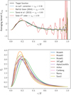 |
Fig. 1 Averaging kernels of the solar model and variation of the target function for a selection of models from our testing set. Top panel: averaging kernels of the solar model by considering different surface effect prescriptions. Bottom panel: variation of the target function of a mean density inversion for a selection of models from our testing set. |
Rejection threshold of the K-flag.
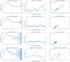 |
Fig. 2 Diagnostic plots of the solar model and of the α Cen A model. From top to bottom: diagnostic plots of the solar model by neglecting the surface effects, using the Ball & Gizon (2014) surface effect prescription, and using a sixth-order polynomial for the surface effects; and diagnostic plots of α Cen A using the Ball & Gizon (2014) prescription. Left column: fit of the target function by the averaging kernel. Central column: inversion coefficients. Right column: lag plot of the inversion coefficients. The points in red are the values that were excluded. |
3.2 R-flag
In a seismic inversion, we assume that the relative frequency differences are independent measurements, but under simplifying hypotheses, one can show that the acoustic frequencies follow an asymptotic relation (Shibahashi 1979; Tassoul 1980):
 (16)
(16)
where ϵ is a phase and ∆y is the large separation. In our previous study (Appendix A of JB23), we noted that the inversion coefficients of a stable inversion tend to show smooth structures. Because of the asymptotic behaviour of the frequencies, the same seismic information can be shared by multiple frequencies and it is therefore not surprising to find smooth structures in the inversion coefficients, as illustrated in Fig. 2 for the solar model. If the target function is less well reproduced by the averaging kernel, these smooth structures break down and the inversion coefficients appear to be more randomly distributed, as illustrated in Fig. 2 for α Cen A. In JB23, we proposed a method to quantify this observation by looking at the lag plot (see e.g. Heckert et al. 2002, for a reference handbook) of the inversion coefficients. Indeed, as shown in the right column of Fig. 2, the inversion coefficients of a stable inversion tend to be positively correlated in the lag plot, assuming a lag of one. In a previous study, we suggested a way to quantify this correlation, namely with the Pearson correlation coefficient (Pearson 1895). However, we found in the present study that this measure is too sensitive to extreme values and is therefore not robust enough for a pipeline implementation. Indeed, one outlier can result in a Pearson coefficient of close to zero, even though all the other points are linearly correlated. We therefore propose the following modifications. We compute the standard deviation of the inversion coefficients and discard the coefficients that are not in the 3cr interval around zero. We chose to centre our interval on zero because this worked well with our testing set by discarding the coefficients that we would have discarded manually. Alternatively, the interval can be centred on the mean of the coefficients, although with a smaller tolerance. We note that if the number of modes becomes low (below 15) or if the inversion is based on the modes of one harmonic degree only, it is preferable to use the second option. Indeed, in such extreme conditions, the first criterion is unreliable and may discard a large fraction of the modes. We also note that up to two coefficients are typically discarded. In general, these correspond to the lowest radial order modes of the harmonic degrees. The correlation of the lag plot is then evaluated with the Spearman correlation coefficient (Spearman 1904). This coefficient focuses on the rank variables R(X) and R(Y) instead of the random variables X and Y themselves. In that regard, the Spearman correlation coefficient is the Pearson correlation coefficient of the rank variables:
 (17)
(17)
This approach is more general; the Spearman coefficient indeed detects a monotonic correlation between the random variables, and has the great advantage of being significantly less sensitive to outliers. We note that if two random variables are linearly correlated, the Pearson and Spearman coefficients are equivalent. Because of these advantages, the Spearman coefficient is more robust and better suited to a pipeline implementation. As in JB23, we identified three regimes, which are summarised in Table 3. We consider that below 𝓡t = 0.4, the inversion coefficients show too much randomness for meaningful inversion. In that case, we reject the inversion result. If 𝓡t > 0.65, we consider that the inversion coefficients form smooth structures and we accept the inversion result. The regime in between these two is more uncertain and we recommend further investigation be carried out. Because this test is based on the inversion coefficients, the boundaries of the different regimes are not dependent on the type of inversion that is considered.
Instability regimes of the R-flag.
4 Results
4.1 Mean density and acoustic radius inversions
The mean density inversion and the acoustic radius inversion are based on the same structural kernels and share the same trade-off parameters. The form of their seismic indicator is simple compared to more ambitious inversions such as the central entropy inversion. Due to these similarities, the results of our quality assessment procedure are very similar. This means that if the mean density inversion is flagged as accepted, the corresponding acoustic radius inversion is typically flagged as accepted too, and vice versa. In this section, we therefore focus our discussion on the results of the mean density inversions, which are displayed in the top line of Fig. 3 and in Table 4, and the results of the acoustic radius inversions can be found in Appendix B.
The results of the calibrator targets are consistent with our expectations. For the solar model, introducing additional free parameters to describe the surface effects increases the value of the  quantifier. The opposite behaviour is observed with the second quantifier, the Spearman correlation coefficient
  . In addition, all these inversions correct towards the expected mean density range. The results for 16 Cyg A and B show a similar behaviour to the results for the Sun. The inversions of both binary components correct towards the measurements of Buldgen et al. (2022)b, and all these inversions are accurately flagged as accepted. In addition, with the high data quality for these targets, both quality quantifiers correctly reflect that the Ball & Gizon (2014) prescription is slightly more stable than the Sonoi et al. (2015) prescription, and that the inversions that neglect surface effects are the most stable. We note that neglecting surface effects gives the most stable inversions because it imposes fewer free variables in the minimisations, but it does not mean that the outcome of this inversion is the best physical result. Indeed, as pointed out by JB23 and by many other studies, the Ball & Gizon (2014) prescription is the best default choice. For the α Cen binary system, we expected poor-quality inversion results. Indeed, the data quality for these targets is lower than the data quality for the other calibrator targets. For these targets, we investigated two types of reference models, that is, with or without overshooting in α Cen A. From the literature, we know that the relative frequency differences of α Cen B are too large for a robust inversion based on individual frequencies, and that the inversion results of the model α Cen A including overshooting are significantly affected by the choice of the mode set, suggesting that some of the modes have a nonlinear character. As expected, the inversions using the sixth-order polynomial to describe the surface effects are rejected. The rest of the inversions are either flagged as rejected or as requiring a manual and thorough investigation. The results for these targets show the relevance of using both quality flags. Indeed, due to the amplitude differences of the target function of models over a large mass range, the fine-tuning of the rejection threshold of the K-flag is limited and would benefit from a lower tolerance for these models in particular. Although the K-flag has a non-negligible false-positive rate, most of these problematic inversions are detected by the second quality flag. In addition, we note that for the model of α Cen A without overshooting and with the Sonoi et al. (2015) surface effects prescription, the inversion result is rejected by the K-flag but not by the R-flag, which illustrates a limitation of the R-flag. If the target function is not reproduced at all by the averaging kernel, the correction proposed by the inversion is non-physical and is the result of the poor fit of the target function. However, it may still create structures in the inversion coefficients that are detected by the R-flag. This is not an issue for our assessment procedure, where the K-flag is first computed. Indeed, if the inversion is rejected by the K-flag, it is unnecessary to compute the R-flag. The quality assessment results of Kepler-93 also correspond to our expectations. The data quality for this target is lower than the data quality for the best Kepler targets with the Ball & Gizon (2014) and Sonoi et al. (2015) prescriptions, and the target function is therefore less well reproduced by the averaging kernel. This is detected by the R-flag, which labelled these inversions as requiring a manual check. The data quality for Kepler-93 is insufficient for surface effect prescriptions with six free variables. This inversion is rejected by the K-flag, but not by the R-flag, which again shows that the R-flag should not be computed for inversion results that were rejected by the K-flag.
The results of the second category of targets are shown in Fig. 3 and in Table 4. The most problematic cases are directly discarded by the K-flag, and the R-flag points out the lower quality inversions. Indeed, by manually checking the fit of the averaging kernel, we identified model B, C, D, and F, and Dushera as lower quality inversions, which are also correctly highlighted by our assessment procedure. The result for Dushera is particularly interesting. Despite having lower data quality than the best targets (e.g. Doris), the data quality is similar to that of other stable inversion results (e.g. Pinocha). However, the inversion result of Dushera is flagged as unreliable. As in the case of α Cen A, it is possible that one (or more) of the modes is affected by non-linearities, which could explain this unstable behaviour. Alternatively, it is also possible that there was an issue with the peak bagging. Indeed, Roxburgh (2017) observed anomalies in some of the LEGACY data. Although the data for Dushera were not analysed in this latter study, it is possible that the data of this target were impacted by the same issues, which could also explain the unstable behaviour of the inversion. Both possibilities could be investigated by a comprehensive analysis using local minimisations, which is beyond the scope of the present study. Nevertheless, this result is promising as it indicates that our assessment procedure is able to highlight problematic inversion results that are usually difficult to detect manually. Additionally, the stable inversion results are correctly flagged as stable. Therefore, we conclude that the combination of both flags performs satisfactorily for the mean density inversion and the acoustic radius inversion and can be considered equivalent to a human modeller.
The Ball & Gizon (2014) prescription is the preferred surface effect prescription for the PLATO pipeline and it is therefore relevant to look at the flag distribution of the inversion results with this prescription. We note that our testing set is not free of bias; we only considered targets with medium- to high-quality data (more than 30 observed modes) and we included several poor-quality inversion results to verify that they could be spotted by our assessment procedure. The percentages that we quote below should therefore be interpreted with caution, and further investigations with larger statistics and including targets of lower data quality are required. With our testing set, about 20% of the results are flagged as rejected, about 20% as ‘to be checked manually’, and the remaining 60% as accepted. Although it is difficult to draw robust conclusions based on these numbers, we note that few inversion results are rejected and also that few results require further investigation. This is an important aspect because such investigations cannot be carried out within the pipeline. These results therefore reassure us that the mean density inversion is suited to large-scale applications.
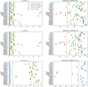 |
Fig. 3 Quality assessment results of the inversion carried out on our testing set by considering different surface effect prescriptions. Left column: quality of the fit of the target function by the averaging kernel quantified by χt. Right column: spearman coefficient ℛt of the lag plot. Top line: results of the mean density inversions. Middle line: results of the acoustic radius inversions. Bottom line: results of the central entropy inversions. The vertical dashed black lines delimit the different regimes of the selection flags. |
Results of our quality assessment procedure applied for the mean density inversions carried out on our testing set.
4.2 Central entropy inversion
The results of the central entropy inversion are shown in the bottom line of Fig. 3 and in Table 5. For all the models, we find that the inversion fails if surface effects are included. Indeed, the inversions using the Ball & Gizon (2014) and Sonoi et al. (2015) prescriptions have averaging kernels that completely miss the central stellar features of the target function. Hence, all these inversion results can be discarded because these central layers are the region of interest of the inversion. In addition, the situation is even worse with the sixth-order polynomial. In this configuration, the number of degrees of freedom is insufficient to carry out the SOLA inversion. As expected, the K-flag rejects all these inversions. Although we recommend avoiding computation of the R-flag for inversions that were rejected by the K-flag, Table 5 provides the R-flag for such models in order to illustrate why we give this recommendation. As shown in Table 5, the R-flag is not reliable in such conditions. Regarding the results of the inversions that neglect surface effects, the performance of our quality assessment procedure is equivalent to that of a human modeller. The models with a lower inversion quality are indeed correctly spotted by the R-flag.
However, these results bring into question the relevance of including this inversion in a pipeline, at least in its current form. This indicator is indeed designed to probe the central stellar layers, but it is also very sensitive to the surface regions because it is based on the S5/3 profile, which is highly sensitive to these regions. Therefore, in order to robustly interpret the results of this type of inversion, it is necessary to generate a set of models that is representative of the observed target and to study the behaviour of the inversion on the set, as is done in (Buldgen et al. 2017a, 2022b) and Salmon et al. (2021), for example. We note that using a similar indicator, but one that is based on frequency separation ratios (Bétrisey & Buldgen 2022), would also be incompatible with a pipeline approach. Even though such an indicator is significantly less affected by surface effects, it is based on ratios that might take very small values and therefore result in singular relative ratio differences. This inversion therefore necessitates some caution in the data processing and in the interpretation of the results. Also, for this inversion, it is still necessary to generate a set of models and to study the inversion's behaviour on the set.
Results of our quality assessment procedure applied for the central entropy inversions carried out on our testing set.
5 Discussion
5.1 Preconditioning of the inversion
The variational inversions are based on a linear formalism. During the derivation of the structure inversion equation at the basis of the variational inversions, this linearity assumption allows us to neglect many higher-order terms − notably surface terms arising from partial integration − and to finally obtain a simple equation directly relating frequency differences to structural differences. Non-linearities may therefore significantly affect the inversion by inducing unwanted compensations, and are usually difficult to spot. In this section, we discuss two types of common non-linearity, the mode non-linearity and the non-linear regime of the reference model.
In the first scenario, the mode itself exhibits a non-linear behaviour. A mixed mode mistaken for a pressure mode fits within this category. This type of non-linearity is often difficult to detect, and in our testing set, we suspect that the model of a Cen A including overshooting is affected by such a non-linearity. For the remaining targets, there is a priori no sign of mode non-linearity. We note that a thorough investigation of each target would be required in order to robustly disprove the presence of such non-linearities, but based on the current inversion results, it is reasonable to assume that such non-linearities only affect a minority of targets and are therefore unlikely to be an issue in a pipeline.
The second scenario is related to the reference model. If this latter is too far away from the observed target in the parameter space, structural differences may be too large for the linear assumption and might induce compensations in the inversion. In Fig. 4, we show the structural differences in density between a model within the linear regime (‘target2NuOv000’), fitting the individual frequencies, and a model outside the linear regime (‘target2R01Ov000’), fitting the r01 ratios alone. We took these models from Bétrisey & Buldgen (2022). In the illustration, ‘target2R01Ov000’ shows large differences in the upper layers, which are magnified by the structural kernels and their large amplitude in these regions; these induce unwanted compensations and the inversion is unsuccessful. The boundaries of the linear regime are often unclear and may change from target to target. However, good preconditioning can ensure that the reference model is in the linear regime. Hence, a fit of the individual frequencies and the classical constraints with an MCMC typically ensures this linear regime configuration. This type of non-linearity is therefore not an issue for the modelling strategy proposed in JB23, which starts with such a fit and then corrects for the surface effects by combining a mean density inversion and a fit of frequency separation ratios.
Assessment flags of the tests on limited mode sets.
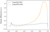 |
Fig. 4 Density differences between two reference models of target 2 from Bétrisey & Buldgen (2022). The reference model 'target2NuOv000' is within the linear regime, while the model 'target2R01Ov000' is outside of the linear regime. |
5.2 Limited mode sets
In Sect. 3, we test our quality assessment procedure on targets with a data quality going from medium to high. This corresponds to mode sets that are composed of more than 30 individual modes. This number of modes allows us to use a statistical tool at the basis of the R-flag. PLATO will however detect many targets with fewer pulsation frequencies. We therefore tested how our assessment procedure behaves in such cases. We investigated three calibrator targets, namely the Sun, Kepler-93, and α Cen A, which are representative of good-, medium-, and poor-quality inversions, respectively.
We summarise the results of our assessment procedure in Table 6. Due to the lower number of modes, we did not discard inversion coefficients above the 3σ threshold used to remove the outliers before the computation of the Spearman correlation coefficient. For the Sun, the inversion is robust if only the l = 0 modes are used (18 modes in total), except for the sixth-order surface effect prescription, as expected. We also tested the performance of the inversion based on ten l = 0 modes around vmax only, and on four modes around vmax of each harmonic degree (12 modes in total). In these conditions, the fit of the target function by the averaging kernel is insufficient and the inversion is rejected by our assessment procedure. For Kepler-93, the quality of the fit of the target function by the averaging kernel with the Ball & Gizon (2014) and Sonoi et al. (2015) prescriptions is in a 'grey zone'. Solely based on this fit, we would have rejected the inversion results. However, based on the inverted mean densities, which are consistent with Bétrisey et al. (2022), and based on the inversion coefficients, which form smooth structures, it seems that these inversions were successful. As expected, these inversions are flagged as accepted by our assessment procedure. Unsurprisingly, for α Cen A – for which poor-quality inversion results were obtained with all the modes –, even poorer quality inversion results were obtained if only the l = 0 modes are used.
Theoretically, an inversion based on a dozen modes is not expected to be challenging, although this is assuming that these modes were carefully selected nonetheless. This is doable in an hare and hounds exercise, but as we show in this section, the outcomes of such inversions are unpredictable. Indeed an actual mode set is composed of the modes that were detected by the instrument, and there is no possibility to carefully select the modes. The inversion carried out on the l = 0 modes of Kepler-93 was successful but there is no guarantee that this will be the case for another target.
6 Conclusions
In Sect. 2, we present the inversion types that we considered in this study and we also present our testing set. In Sect. 3, we describe our quality assessment procedure, which we applied to our testing set in Sect. 4. Finally in Sect. 5, we discuss the best practices required in order to carry out the large-scale application of our assessment procedure.
Even though the mean density inversion (Reese et al. 2012) and the acoustic radius inversion (Buldgen et al. 2015b) were originally developed for individual modelling, the results of JB23 and of this study reinforce our belief that these inversions are compatible with large-scale application. The central entropy inversion (Buldgen et al. 2018), which is based on a seismic indicator with a more complex form, is nevertheless not compatible with large-scale application in its current form. We find that our procedure performs as well as a human modeller. Nonetheless, we note that we mainly tested our procedure on targets for which medium- to high-quality data are available and which have least at 30 observed modes. Dealing with lower statistics may be an issue for the second test of our procedure, but not for the first test. In this regard, we believe that our procedure is still applicable to limited mode sets, although this aspect would benefit from further investigation. However, a limited mode set of a dozen frequencies could be an issue for the inversion itself. Indeed, the kernels of such mode sets may be insufficient for the averaging kernel to reproduce the target function. In these conditions, the success of an inversion becomes unpredictable and is sensitive to the mode set that is used.
Putting these results in the context of the PLATO mission, our quality assessment procedure of seismic inversions shows promising results. It is indeed based on the by-products of the inversion, and the two quality tests that are performed require few numerical resources. Hence, our assessment procedure can assess the quality of an inversion quickly and inexpensively, while still performing as well as a human modeller.
Acknowledgements
J.B. and G.B. acknowledge funding from the SNF AMBIZIONE grant No 185805 (Seismic inversions and modelling of transport processes in stars). G.M. has received funding from the European Research Council (ERC) under the European Union's Horizon 2020 research and innovation programme (grant agreement No 833925, project STAREX). Finally, this work has benefited from financial support by CNES (Centre National des Etudes Spatiales) in the framework of its contribution to the PLATO mission.
Appendix A Supplementary data for K-flag
In Fig. A.1, we show illustrations of outliers that are directly rejected by the first flag of our quality assessment procedure.
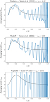 |
Fig. A.1 Outlying cases where the averaging kernel is unable to reproduce the target function. The |

Appendix B Assessment flags of the acoustic radius inversions
Table B.1 shows the assessment flags of the acoustic inversions carried out on our testing set. As mentioned in Sect. 4.1, the quality behaviour of a mean density inversion is similar to that of an acoustic radius inversion. We therefore invite the reader to refer to this section for the interpretation of the results.
Results of our quality assessment procedure applied for the acoustic radius inversions carried out on our testing set.
References
- Backus, G., & Gilbert, F. 1968, Geophys. J., 16, 169 [NASA ADS] [CrossRef] [Google Scholar]
- Backus, G., & Gilbert, F. 1970, Philos. Trans. R. Soc. London Ser. A, 266, 123 [NASA ADS] [CrossRef] [Google Scholar]
- Baglin, A., Auvergne, M., Barge, P., et al. 2009, IAU Symp., 253, 71 [Google Scholar]
- Ball, W. H., & Gizon, L. 2014, A&A, 568, A123 [NASA ADS] [CrossRef] [EDP Sciences] [Google Scholar]
- Ball, W. H., & Gizon, L. 2017, A&A, 600, A128 [NASA ADS] [CrossRef] [EDP Sciences] [Google Scholar]
- Basu, S., & Antia, H. M. 2008, Phys. Rep., 457, 217 [Google Scholar]
- Basu, S., & Christensen-Dalsgaard, J. 1997, A&A, 322, L5 [NASA ADS] [Google Scholar]
- Basu, S., Christensen-Dalsgaard, J., Perez Hernandez, F., & Thompson, M. J. 1996, MNRAS, 280, 651 [NASA ADS] [Google Scholar]
- Bellinger, E. P., Basu, S., Hekker, S., & Ball, W. H. 2017, ApJ, 851, 80 [NASA ADS] [CrossRef] [Google Scholar]
- Bellinger, E. P., Hekker, S., Angelou, G. C., Stokholm, A., & Basu, S. 2019, A&A, 622, A130 [NASA ADS] [CrossRef] [EDP Sciences] [Google Scholar]
- Bellinger, E. P., Basu, S., Hekker, S., Christensen-Dalsgaard, J., & Ball, W. H. 2021, ApJ, 915, 100 [NASA ADS] [CrossRef] [Google Scholar]
- Bétrisey, J., & Buldgen, G. 2022, A&A, 663, A92 [NASA ADS] [CrossRef] [EDP Sciences] [Google Scholar]
- Bétrisey, J., Pezzotti, C., Buldgen, G., et al. 2022, A&A, 659, A56 [NASA ADS] [CrossRef] [EDP Sciences] [Google Scholar]
- Bétrisey, J., Buldgen, G., Reese, D. R., et al. 2023a, A&A, 676, A10 [NASA ADS] [CrossRef] [EDP Sciences] [Google Scholar]
- Bétrisey, J., Eggenberger, P., Buldgen, G., Benomar, O., & Bazot, M. 2023b, A&A, 673, L11 [NASA ADS] [CrossRef] [EDP Sciences] [Google Scholar]
- Borucki, W. J., Koch, D., Basri, G., et al. 2010, Science, 327, 977 [Google Scholar]
- Broomhall, A. M., Chaplin, W. J., Elsworth, Y., & New, R. 2011, MNRAS, 413, 2978 [NASA ADS] [CrossRef] [Google Scholar]
- Buldgen, G., Reese, D. R., & Dupret, M. A. 2015a, A&A, 583, A62 [NASA ADS] [CrossRef] [EDP Sciences] [Google Scholar]
- Buldgen, G., Reese, D. R., Dupret, M. A., & Samadi, R. 2015b, A&A, 574, A42 [NASA ADS] [CrossRef] [EDP Sciences] [Google Scholar]
- Buldgen, G., Reese, D. R., & Dupret, M. A. 2016a, A&A, 585, A109 [NASA ADS] [CrossRef] [EDP Sciences] [Google Scholar]
- Buldgen, G., Salmon, S. J. A. J., Reese, D. R., & Dupret, M. A. 2016b, A&A, 596, A73 [NASA ADS] [CrossRef] [EDP Sciences] [Google Scholar]
- Buldgen, G., Reese, D., & Dupret, M.-A. 2017a, Euro. Phys. J. Conf., 160, 03005 [CrossRef] [EDP Sciences] [Google Scholar]
- Buldgen, G., Reese, D. R., & Dupret, M. A. 2017b, A&A, 598, A21 [NASA ADS] [CrossRef] [EDP Sciences] [Google Scholar]
- Buldgen, G., Reese, D. R., & Dupret, M. A. 2018, A&A, 609, A95 [NASA ADS] [CrossRef] [EDP Sciences] [Google Scholar]
- Buldgen, G., Farnir, M., Pezzotti, C., et al. 2019a, A&A, 630, A126 [EDP Sciences] [Google Scholar]
- Buldgen, G., Rendle, B., Sonoi, T., et al. 2019b, MNRAS, 482, 2305 [Google Scholar]
- Buldgen, G., Salmon, S., & Noels, A. 2019c, Front. Astron. Space Sci., 6, 42 [NASA ADS] [CrossRef] [Google Scholar]
- Buldgen, G., Bétrisey, J., Roxburgh, I. W., Vorontsov, S. V., & Reese, D. R. 2022a, Front. Astron. Space Sci., 9, 942373 [NASA ADS] [CrossRef] [Google Scholar]
- Buldgen, G., Farnir, M., Eggenberger, P., et al. 2022b, A&A, 661, A143 [NASA ADS] [CrossRef] [EDP Sciences] [Google Scholar]
- Chandrasekhar, S. 1964, ApJ, 139, 664 [Google Scholar]
- Chandrasekhar, S., & Lebovitz, N. R. 1964, ApJ, 140, 1517 [NASA ADS] [CrossRef] [Google Scholar]
- Christensen-Dalsgaard, J. 2021, Liv. Rev. Sol. Phys., 18, 2 [NASA ADS] [CrossRef] [Google Scholar]
- Christensen-Dalsgaard, J., Schou, J., & Thompson, M. J. 1990, MNRAS, 242, 353 [NASA ADS] [Google Scholar]
- Clement, M. J. 1964, ApJ, 140, 1045 [NASA ADS] [CrossRef] [Google Scholar]
- Cunha, M. S., Roxburgh, I. W., Aguirre Børsen-Koch, V., et al. 2021, MNRAS, 508, 5864 [NASA ADS] [CrossRef] [Google Scholar]
- de Meulenaer, P., Carrier, F., Miglio, A., et al. 2010, A&A, 523, A54 [NASA ADS] [CrossRef] [EDP Sciences] [Google Scholar]
- di Mauro, M. P. 2004, ESA SP, 559, 186 [Google Scholar]
- Dziembowski, W. A., Pamyatnykh, A. A., & Sienkiewicz, R. 1990, MNRAS, 244, 542 [NASA ADS] [Google Scholar]
- Elliott, J. R. 1996, MNRAS, 280, 1244 [NASA ADS] [CrossRef] [Google Scholar]
- Frandsen, S., Carrier, F., Aerts, C., et al. 2002, A&A, 394, L5 [NASA ADS] [CrossRef] [EDP Sciences] [Google Scholar]
- Furlan, E., Ciardi, D. R., Cochran, W. D., et al. 2018, ApJ, 861, 149 [Google Scholar]
- Gough, D. 1985, Sol. Phys., 100, 65 [NASA ADS] [CrossRef] [Google Scholar]
- Gough, D. O. 1993, in Astrophysical Fluid Dynamics - Les Houches 1987 (Cambridge: Cambridge University Press), 399 [Google Scholar]
- Gough, D. O., & Thompson, M. J. 1991, The inversion problem (Tucson: The University of Arizona Press), 519 [Google Scholar]
- Heckert, N., Filliben, J., Croarkin, C., et al. 2002, Handbook 151: NIST/SEMATECH e-Handbook of Statistical Methods (Gaithersburg: NIST) [Google Scholar]
- Howe, R., Chaplin, W. J., Basu, S., et al. 2020, MNRAS, 493, L49 [Google Scholar]
- Huber, D., Ireland, M. J., Bedding, T. R., et al. 2012, ApJ, 760, 32 [Google Scholar]
- Jørgensen, A. C. S., Montalbán, J., Miglio, A., et al. 2020, MNRAS, 495, 4965 [CrossRef] [Google Scholar]
- Jørgensen, A. C. S., Montalbán, J., Angelou, G. C., et al. 2021, MNRAS, 500, 4277 [Google Scholar]
- Kjeldsen, H., Bedding, T. R., Butler, R. P., et al. 2005, ApJ, 635, 1281 [NASA ADS] [CrossRef] [Google Scholar]
- Kjeldsen, H., Bedding, T. R., & Christensen-Dalsgaard, J. 2008, ApJ, 683, L175 [Google Scholar]
- Kosovichev, A. G. 1999, J. Comput. Appl. Math., 109, 1 [NASA ADS] [CrossRef] [Google Scholar]
- Kosovichev, A. G. 2011, in Lect. Notes Phys., eds. J.-P. Rozelot, & C. Neiner (Berlin Heidelberg: Springer), 832, 3 [NASA ADS] [CrossRef] [Google Scholar]
- Kosovichev, A. G., & Kitiashvili, I. N. 2020, IAU Symp., 354, 107 [NASA ADS] [Google Scholar]
- Lin, C.-H., & Däppen, W. 2005, ApJ, 623, 556 [NASA ADS] [CrossRef] [Google Scholar]
- Lund, M. N., Silva Aguirre, V., Davies, G. R., et al. 2017, ApJ, 835, 172 [Google Scholar]
- Lynden-Bell, D., & Ostriker, J. P. 1967, MNRAS, 136, 293 [Google Scholar]
- Metcalfe, T. S., Chaplin, W. J., Appourchaux, T., et al. 2012, ApJ, 748, L10 [Google Scholar]
- Miglio, A., & Montalbán, J. 2005, A&A, 441, 615 [NASA ADS] [CrossRef] [EDP Sciences] [Google Scholar]
- Nsamba, B., Campante, T. L., Monteiro, M. J. P. F. G., et al. 2018, MNRAS, 477, 5052 [NASA ADS] [CrossRef] [Google Scholar]
- Pearson, K. 1895, Proc. R. Soc. London, 58, 240 [NASA ADS] [CrossRef] [Google Scholar]
- Pijpers, F. P. 2006, Methods in Helio- and Asteroseismology (UK: Imperial College Press) [CrossRef] [Google Scholar]
- Pijpers, F. P., & Thompson, M. J. 1992, A&A, 262, L33 [NASA ADS] [Google Scholar]
- Pijpers, F. P., & Thompson, M. J. 1994, A&A, 281, 231 [NASA ADS] [Google Scholar]
- Pijpers, F. P., Teixeira, T. C., Garcia, P. J., et al. 2003, A&A, 406, L15 [NASA ADS] [CrossRef] [EDP Sciences] [Google Scholar]
- Prša, A., Harmanec, P., Torres, G., et al. 2016, AJ, 152, 41 [Google Scholar]
- Rabello-Soares, M. C., Basu, S., & Christensen-Dalsgaard, J. 1999, MNRAS, 309, 35 [NASA ADS] [CrossRef] [Google Scholar]
- Ramírez, I., Meléndez, J., & Asplund, M. 2009, A&A, 508, L17 [NASA ADS] [CrossRef] [EDP Sciences] [Google Scholar]
- Rauer, H., Catala, C., Aerts, C., et al. 2014, Exp. Astron., 38, 249 [Google Scholar]
- Reese, D. R., Marques, J. P., Goupil, M. J., Thompson, M. J., & Deheuvels, S. 2012, A&A, 539, A63 [NASA ADS] [CrossRef] [EDP Sciences] [Google Scholar]
- Ricker, G. R., Winn, J. N., Vanderspek, R., et al. 2015, J. Astron. Teles. Instrum. Syst., 1, 014003 [Google Scholar]
- Roxburgh, I. W. 2017, A&A, 604, A42 [NASA ADS] [CrossRef] [EDP Sciences] [Google Scholar]
- Salabert, D., García, R. A., & Turck-Chièze, S. 2015, A&A, 578, A137 [NASA ADS] [CrossRef] [EDP Sciences] [Google Scholar]
- Salmon, S. J. A. J., Van Grootel, V., Buldgen, G., Dupret, M. A., & Eggenberger, P. 2021, A&A, 646, A7 [NASA ADS] [CrossRef] [EDP Sciences] [Google Scholar]
- Santos, A. R. G., Campante, T. L., Chaplin, W. J., et al. 2018, ApJS, 237, 17 [NASA ADS] [CrossRef] [Google Scholar]
- Santos, A. R. G., Campante, T. L., Chaplin, W. J., et al. 2019a, ApJ, 883, 65 [CrossRef] [Google Scholar]
- Santos, A. R. G., García, R. A., Mathur, S., et al. 2019b, ApJS, 244, 21 [Google Scholar]
- Santos, A. R. G., Breton, S. N., Mathur, S., & García, R. A. 2021, ApJS, 255, 17 [NASA ADS] [CrossRef] [Google Scholar]
- Sekii, T. 1997, in Sounding Solar and Stellar Interiors, eds. J. Provost, & F.-X. Schmider (Cambridge: Cambridge University Press), 181 [Google Scholar]
- Shibahashi, H. 1979, PASJ, 31, 87 [NASA ADS] [Google Scholar]
- Sonoi, T., Samadi, R., Belkacem, K., et al. 2015, A&A, 583, A112 [NASA ADS] [CrossRef] [EDP Sciences] [Google Scholar]
- Spearman, C. 1904, Am. J. Psychol., 15, 72 [Google Scholar]
- Tassoul, M. 1980, ApJS, 43, 469 [Google Scholar]
- Teixeira, T. C., Christensen-Dalsgaard, J., Carrier, F., et al. 2003, Ap&SS, 284, 233 [NASA ADS] [CrossRef] [Google Scholar]
- Thomas, A. E. L., Chaplin, W. J., Basu, S., et al. 2021, MNRAS, 502, 5808 [NASA ADS] [CrossRef] [Google Scholar]
- Tikhonov, A. N. 1963, Sov. Math. Dokl., 4, 1035 [Google Scholar]
- White, T. R., Huber, D., Maestro, V., et al. 2013, MNRAS, 433, 1262 [Google Scholar]
All Tables
Results of our quality assessment procedure applied for the mean density inversions carried out on our testing set.
Results of our quality assessment procedure applied for the central entropy inversions carried out on our testing set.
Results of our quality assessment procedure applied for the acoustic radius inversions carried out on our testing set.
All Figures
|
Fig. 1 Averaging kernels of the solar model and variation of the target function for a selection of models from our testing set. Top panel: averaging kernels of the solar model by considering different surface effect prescriptions. Bottom panel: variation of the target function of a mean density inversion for a selection of models from our testing set. |
| In the text | |
|
Fig. 2 Diagnostic plots of the solar model and of the α Cen A model. From top to bottom: diagnostic plots of the solar model by neglecting the surface effects, using the Ball & Gizon (2014) surface effect prescription, and using a sixth-order polynomial for the surface effects; and diagnostic plots of α Cen A using the Ball & Gizon (2014) prescription. Left column: fit of the target function by the averaging kernel. Central column: inversion coefficients. Right column: lag plot of the inversion coefficients. The points in red are the values that were excluded. |
| In the text | |
|
Fig. 3 Quality assessment results of the inversion carried out on our testing set by considering different surface effect prescriptions. Left column: quality of the fit of the target function by the averaging kernel quantified by χt. Right column: spearman coefficient ℛt of the lag plot. Top line: results of the mean density inversions. Middle line: results of the acoustic radius inversions. Bottom line: results of the central entropy inversions. The vertical dashed black lines delimit the different regimes of the selection flags. |
| In the text | |
|
Fig. 4 Density differences between two reference models of target 2 from Bétrisey & Buldgen (2022). The reference model 'target2NuOv000' is within the linear regime, while the model 'target2R01Ov000' is outside of the linear regime. |
| In the text | |
|
Fig. A.1 Outlying cases where the averaging kernel is unable to reproduce the target function. The |
| In the text | |
Current usage metrics show cumulative count of Article Views (full-text article views including HTML views, PDF and ePub downloads, according to the available data) and Abstracts Views on Vision4Press platform.
Data correspond to usage on the plateform after 2015. The current usage metrics is available 48-96 hours after online publication and is updated daily on week days.
Initial download of the metrics may take a while.