| Issue |
A&A
Volume 677, September 2023
|
|
|---|---|---|
| Article Number | A125 | |
| Number of page(s) | 12 | |
| Section | Extragalactic astronomy | |
| DOI | https://doi.org/10.1051/0004-6361/202347294 | |
| Published online | 15 September 2023 | |
The contribution of faint Lyman-α emitters to extended Lyman-α halos constrained by MUSE clustering measurements
1
Leibniz-Institut für Astrophysik Potsdam (AIP), An der Sternwarte 16, 14482 Potsdam, Germany
e-mail: yherreroalonso@aip.de
2
Universidad Nacional Autónoma de México, Instituto de Astronomía (IA-UNAM-E), AP 106, Ensenada, 22860 BC, Mexico
3
Leiden Observatory, Leiden University, PO Box 9513 2300 RA Leiden, The Netherlands
Received:
27
June
2023
Accepted:
31
July
2023
Recent detections of extended Lyman-α halos around Lyα emitters (LAEs) have been reported on a regular basis, but their origin is still under investigation. Simulation studies predict that the outer regions of the extended halos contain a major contribution from the Lyα emission of faint, individually undetected LAEs. To address this matter from an observational angle, we used halo occupation distribution (HOD) modeling to reproduce the clustering of a spectroscopic sample of 1265 LAEs at 3 < z < 5 from the MUSE-Wide survey. We integrated the Lyα luminosity function to estimate the background surface brightness due to discrete faint LAEs. We then extended the HOD statistics inwards towards small separations and computed the factor by which the measured Lyα surface brightness is enhanced by undetected close physical neighbors. We considered various clustering scenarios for the undetected sources and compared the corresponding radial profiles. This enhancement factor from LAE clustering depends strongly on the spectral bandwidth Δv over which the Lyα emission is integrated and this value can amount to ≈20 − 40 for small values of Δv (around 200 − 400 km s−1) as achieved by recent studies utilizing integral-field spectrographic data. The resulting inferred Lyα surface brightness of faint LAEs ranges between (0.4 − 2)×1020 erg s−1 cm−2 arcsec−2, with a very slow radial decline outwards. Our results suggest that the outer regions of observed Lyα halos (R ≳ 50 pkpc) could indeed contain a strong component from external (but physically associated) LAEs, and may even be dominated by them. It is only for a relatively shallow faint-end slope of the Lyα luminosity function that this contribution from clustered LAEs would be rendered insignificant. We also confirm that the observed emission from the inner regions (R ≤ 20 − 30 pkpc) is too bright to be substantially affected by clustering. We compare our findings with predicted profiles from simulations and find good overall agreement. We outline possible future measurements to further constrain the impact of discrete undetected LAEs on observed extended Lyα halos.
Key words: galaxies: high-redshift / galaxies: evolution / galaxies: halos / large-scale structure of Universe / cosmology: observations
© The Authors 2023
 Open Access article, published by EDP Sciences, under the terms of the Creative Commons Attribution License (https://creativecommons.org/licenses/by/4.0), which permits unrestricted use, distribution, and reproduction in any medium, provided the original work is properly cited.
This article is published in open access under the Subscribe to Open model. Subscribe to A&A to support open access publication.
1. Introduction
The Lyα line is a paramount cosmological feature for probing early star-forming galaxies and commonly assists in the detection of high-redshift galaxies, namely, Lyα emitters (LAEs). The ionizing photons produced by their young stars ionize neutral hydrogen (H I) atoms in the neighbouring interstellar medium (ISM) and, after recombination, they have a probability of about 65% of being re-emitted as Lyα photons (Partridge & Peebles 1967). As a result of the complex radiative transfer that the Lyα emission undergoes, a fraction of photons escape the ISM by resonantly scattering with H I throughout the circumgalactic and intergalactic media (CGM, IGM). In combination with several other factors, this effect causes the emission to become diffuse, giving rise to so-called extended Lyα halos.
Statistically relevant detections of extended Lyα halos (LAHs) have employed narrowband imaging observations (Hayashino et al. 2004; Nilsson et al. 2009; Finkelstein et al. 2011), which restrained the detectable surface brightness (SB) level to ∼10−18 erg s−1 cm−2 arcsec−2. A significant step forward in terms of limiting SB is demonstrated in the studies of Steidel et al. (2011), Matsuda et al. (2012), Momose et al. (2014), Xue et al. (2017), who adopted the image-stacking approach and extended the SB threshold by an order of magnitude, SB ∼ 10−19 erg s−1 cm−2 arcsec−2. Recently, another major sensitivity improvement was made possible by the Multi-Unit Spectroscopic Explorer (MUSE) instrument at the ESO-VLT (Bacon et al. 2010), which evened out the limiting SB of individual object-by-object measurements to the limits obtained by the stacking of narrowband data. Wisotzki et al. (2016), Leclercq et al. (2017), Claeyssens et al. (2022), Kusakabe et al. (2022) reported the detection of ubiquitous extended LAHs at 3 < z < 6 and found that, on average, the LAHs detected by MUSE are a factor 4 − 20 more extended than their corresponding UV galaxy sizes, presenting median scale lengths of few physical kpc (pkpc). Combining the added depth of MUSE and the signal gain through stacking, Wisotzki et al. (2018) ascertained extended LAHs at much larger scales (≈60 pkpc at z = 3) than previous studies at similar redshifts (≈30 pkpc). Recent works with Hobby-Eberly Telescope Dark Energy Experiment (HETDEX; Gebhardt et al. 2021) LAEs at 1.9 < z < 3.5 and Subaru LAEs at z = 2.2 − 2.3 again roughly doubled the radii over which LAHs can be detected (160 pkpc and 200 pkpc, respectively; Niemeyer et al. 2022; Zhang et al. 2023).
Understanding the characteristics and, in particular, the nature of these extended LAHs provides information as to the spatial distribution and kinematic properties of the CGM (Zheng et al. 2011) as well as, more fundamentally, to the processes of formation and evolution of galaxies (Bahcall & Spitzer 1969). The main mechanisms that are believed to contribute to the existence of LAHs are (i) resonant scattering of Lyα photons produced in ionized H II regions of the ISM, (ii) “in situ” recombination, (iii) fluorescence by photons from the metagalactic UV background, and (iv) collisional excitation from cooling gas accreted onto galaxies, also denoted as “gravitational cooling”. Processes (i) and (ii) are consequences of local star formation through Lyman continuum radiation emitted from young and massive stars in star-forming galaxies: processes (iii) and (iv) are driven by external influences.
Comparisons between observational constraints and simulation studies have not yet delivered unique conclusions about the dominant origin of LAHs. Furthermore, while some simulation studies (e.g., Dijkstra & Kramer 2012; Gronke & Bird 2017) were able to fully explain the observed extended Lyα emission with the processes mentioned above, others (Shimizu & Umemura 2010; Lake et al. 2015; Mas-Ribas & Dijkstra 2016; Mas-Ribas et al. 2017; Mitchell et al. 2021; Byrohl et al. 2021) argued that in addition to these factors there is a significant contribution from Lyα emission originating in faint satellite galaxies. This emission would be significant only by its collective effects, as most of these “satellite LAEs” are too faint to be detected individually at the sensitivity of current observations. Lake et al. (2015) assessed that in their simulations the cooling of gas accreted onto galaxies as well as nebular radiation from satellites are the major contributors in the outer halo (R > 2 pkpc). Mitchell et al. (2021) found that scattering is the dominant mechanism in the inner regions of the SB profile (R < 7 pkpc, SB of few SB ∼ 10−19 erg s−1 cm−2), scattering and satellites contribute equally at intermediate scales (R ≈ 10 pkpc, SB ∼ 10−19 erg s−1 cm−2), and satellites dominate the large scales (R > 20 pkpc, SB ∼ 10−20 erg s−1 cm−2 arcsec−2). Similar conclusions were drawn in Byrohl et al. (2021), whereby the authors identified scattering as the major source of SB and held photons originating in dark matter halos (DMHs) in the vicinity of the central galaxy responsible for the flattening of the observed SB profiles at R > 100 pkpc.
The existence of faint sources around more massive and brighter galaxies is certainly predicted by the hierarchical cold dark matter (CDM) model of structure formation. Because this is closely related to non-linear clustering, Mas-Ribas et al. (2017) considered several clustering scenarios, coupled to the analytic formalism described in Mas-Ribas & Dijkstra (2016), to investigate the plausibility of faint sources generating LAHs. In line with the previously mentioned simulations, they found that faint LAEs are the major contributors to the Lyα SB profiles already at R > 4 pkpc. In contrast, Kakiichi & Dijkstra (2018) applied a model based on galaxy-Lyα forest clustering data to build Lyα SB profiles that could match a multitude of observed Lyα SB profiles even without considering the contribution from faint LAEs.
Despite the theoretical efforts to distinguish between the numerous contributions to the extended LAHs, observational tests and evidence for the “faint LAE” scenario are scant, mainly because of the extremely low SB of the Lyα emission at large distances from galaxies. Bacon et al. (2021) detected very extended Lyα emission around LAE overdensities in the MUSE extremely deep field (MXDF), reaching far beyond individual LAHs, but from comparing their data with the semi-analytic model GALICS (Garel et al. 2015) they concluded that much (and possibly all) of the apparently diffuse emission can be accounted for by the collective contribution of discrete faint LAEs surrounding more luminous (detected) ones.
A key step that is still missing is an assessment of the magnitude of this contribution based on observations, rather than on theoretical predictions. In this paper, we address this issue by employing LAE clustering statistics in combination with halo occupation distribution (HOD) models to obtain observational constraints on the contribution of the faint LAEs to the extended LAHs. We built on our previous study (Herrero Alonso et al. 2023, hereafter HA23), where we used the HOD framework to interpret the clustering of three MUSE LAE samples at 3 < z < 6. Each dataset had a different exposure time and thus covered a distinct range of Lyα luminosities within 40.15 < log(LLyα/[erg s−1]) < 43.35. We found a strong (8σ significance) clustering dependence on LLyα, where more luminous LAEs cluster more strongly and reside in more massive DMHs than faint LAEs.
The paper is structured as follows. In Sect. 2, we briefly describe the data used for this work. In Sect. 3, we summarize the clustering properties of our galaxy sample. We extrapolate the clustering features to estimate the contribution of undetected LAEs to the extended Lyα halos in Sect. 4, where we also compare our estimations to recent observational and simulated results. We give our conclusions in Sect. 5.
Throughout the paper, co-moving and physical distances are given in units of h−1 Mpc and pkpc, respectively, where h = H0/100 = 0.70. We use a ΛCDM cosmology and adopt ΩM = 0.3, ΩΛ = 0.7, and σ8 = 0.8 (Hinshaw et al. 2013). All uncertainties represent 1σ (68.3%) confidence intervals.
2. Data
This paper is based on the results from two different spectroscopic MUSE samples. We used a sample of LAEs from the MUSE-Wide survey for the clustering constraints and we employed the data from two MUSE deep fields for the comparison to observed Lyα halos (see Sect. 4.4).
2.1. The MUSE-Wide survey
The main input to the HOD model of Sect. 3 is based on the clustering constraints of a subset of the LAE MUSE-Wide survey (Herenz et al. 2017; Urrutia et al. 2019), which is similar to the LAE dataset used in Herrero Alonso et al. (2023). The sample is constructed from 100 fields, each spanning 1 arcmin2, observed with an exposure time of one hour, and covering regions of CANDELS/GOODS-S, CANDELS/COSMOS and the Hubble Ultra Deep Field (HUDF) parallel fields. The survey also incorporates shallow (1.6 h) subsets of MUSE-Deep data (Bacon et al. 2017, 2022) within the HUDF in the CANDELS/GOODS-S region. We refer to Urrutia et al. (2019) for further details on survey build-up, reduction, and flux calibration of the MUSE data cubes.
In contrast to the study in HA23, here we focus on LAEs with redshifts within 3 < z < 5 (and use the same redshift interval for the comparison to Lyα SB profile measurements in Sect. 4.4). Because Lyα peak redshifts are typically offset by up to several hundreds of km s−1 from systemic ones (e.g., Hashimoto et al. 2015; Muzahid et al. 2020; Schmidt et al. 2021), we corrected the Lyα redshifts following the relations given in Verhamme et al. (2018), which assure an accuracy of ≤100 km s−1 (Schmidt et al. 2021). We refer to Herrero Alonso et al. (2021, hereafter HA21), and references therein for further details on the LAE sample construction.
Our sample comprises a total of 1265 LAEs with Lyα luminosities in the range 40.84 < log(LLyα/[erg s−1]) < 43.30 and a median value of ⟨log(LLyα/[erg s−1])⟩ = 42.27. While the Lyα luminosity and redshift distributions of the sample are presented in Fig. 1, Figs. 1 and B.1 of HA23 show the spatial coverage of the LAE dataset. Taking into account the field-to-field overlaps, the actual surveyed area corresponds to 90.2 arcmin2 and extends ≈43 h−1 Mpc at the median redshift of the sample ⟨z⟩ = 3.8. This implies a LAE density of ≃2 × 10⁻³ h3 Mpc−3.
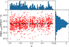 |
Fig. 1. Distribution in Lyα luminosity-redshift space of the 3 < z < 5 LAEs selected from the spectroscopic MUSE-Wide survey. The dashed line corresponds to the median log LLyα of the sample. The normalized redshift and log LLyα distributions are shown in the top and right panels, respectively. |
2.2. MUSE Deep fields
In Sect. 4.4, we compare our results to Lyα radial SB profiles, using the same data and measured in a similar way as by Wisotzki et al. (2018). The parent sample is a combination of LAEs detected by MUSE in the Hubble Deep Field South (Bacon et al. 2015) and in the Hubble Ultra-Deep Field (Bacon et al. 2017), as well as the definition of the final sample proceeds as in Wisotzki et al. (2018), with the exception that here we are only considering a single set of objects with redshifts of 3 < z < 5.
To further facilitate a comparison to the clustering predictions, we also modified the construction of the resulting Lyα SB profile as follows: instead of the individually optimized spectral extraction windows for each LAE used by Wisotzki et al. (2018), we adopted a fixed velocity bandwidth of 600 km s−1 centered on the peak of the Lyα emission of each galaxy. This bandwidth not only provides a good compromise between noise suppression and flux loss avoidance in the stacking approach, it also facilitates the redshift-space distortion modeling (described in Sect. 3). We denote the individually extracted Lyα images as “pseudo-narrowband” in order to distinguish then from genuine filter-based narrowband (NB) imaging data, which encompass much wider bandwidths of typically ≈12 000 − 25 000 km s−1. Unlike Wisotzki et al. (2018), we also skipped the artificial truncation of the used pseudo-NB data at a radius of 6′ (≈40 kpc), and we now used the mean instead of the median to stack the images, to make the resulting profiles as similar as possible to the clustering calculations in their construction logic.
3. Clustering framework
In HA23 we measured the clustering of three LAE samples, including a subset of the MUSE-Wide survey, with the K-estimator of Adelberger et al. (2005). The K-estimator measures the radial clustering along line of sight distance, Z, by counting galaxy pairs in redshift space at fixed transverse separations, R. The K-estimator is directly related to the average underlying correlation function (see Eq. (2) in HA21). We refer to Sect. 3.1 in HA21 for further details.
We then fitted the K-estimator measurements with HOD modeling performed at the median redshift of the galaxy pairs of the sample. The HOD model we used is a simplified version of the five parameter model by Zheng et al. (2007). Because of sample size limitations, the halo mass at which the satellite occupation becomes zero and the scatter in the central halo occupation lower mass cutoff were fixed to M0 = 0 and σlog M = 0, respectively. The three free parameters are then the minimum halo mass required to host a central galaxy, Mmin, the halo mass threshold to host (on average) one satellite galaxy, M1, and the high-mass power-law slope of the satellite galaxy mean occupation function, α (see Sect. 3.3 in HA23). Although we included redshift space distortions (RSDs) in the two-halo term using linear theory (Kaiser infall, Kaiser 1987; van den Bosch et al. 2013), we ignored the effect of RSDs in the one-halo term given its negligible effect at the scales there considered.
The most relevant finding of HA23 for this work is the strong clustering dependence on Lyα luminosity. Luminous (log(LLyα/[erg s−1]) ≈ 42.53) LAEs cluster significantly (8σ) more strongly and reside in ≈25 times more massive DMHs than less luminous (log(LLyα/[erg s−1]) ≈ 40.97) LAEs. Hence, any fainter dataset is assumed to be less strongly clustered than those considered here or in HA23.
In Appendix A, we demonstrate that the clustering strengths of the MUSE-Wide LAE subset considered in HA23 and our current sample are nearly identical. We convert the best-fit HOD model of the K-estimator found in HA23 to the traditional real-space two-point correlation function (2pcf) using Eq. (2) in HA21. In the left panel of Fig. 2 we represent the real-space 2pcf, ξ(r), where  , and where the contours show the expected circular symmetry. The model parameters correspond to a minimum DMH mass for central LAEs of log(Mmin/[h−1 M⊙]) = 10.7, a threshold DMH mass for satellite LAEs of log(M1/[h−1 M⊙]) = 12.4 and a power-law slope of the number of satellites α = 2.8. The corresponding satellite fraction, typical DMH mass, and virial radius are fsat ≈ 0.012,
 ![$ \log (M_{\mathrm{h}}/[h^{-1}\,{M}_\odot])=11.09^{+0.10}_{-0.09} $](/articles/aa/full_html/2023/09/aa47294-23/aa47294-23-eq2.gif) , and
, and  kpc, respectively (HA23).
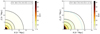 |
Fig. 2. Best-fit HOD modeled real- and redshift-space 2pcf. Left: real-space 2pcf, ξ(r), for the sample of MUSE-Wide LAEs at 3 < z < 5. Note: the circular symmetry of the color-coded contours. Right: redshift-space 2pcf, ξ(s). The dotted blue contours show the real-space 2pcf from the left panel. Note: the elongation of the 2pcf contours along the line-of-sight direction, Zs, at small scales (FoG effect) and the flattening at larger transverse separations, R, (Kaiser infall). The contour levels are indicated in the legend. |
Given the small bandwidths of the extracted pseudo-NB Lyα images from MUSE data (a few hundred km s−1 or few comoving Mpc), we then included RSDs in the one-halo term (the so-called Fingers of God effect, FoG), following Tinker (2007). We convolved the line of sight component of the real-space 2pcf with the probability distribution function of galaxy pairwise velocities, P(v). For each DMH mass, Mh, we assume a Gaussian distribution P(v, Mh) with velocity dispersion of central-satellite pairs determined by the streaming model namely,  , where Rvir is the virial radius. A Gaussian P(v, Mh) is supported by hydrodynamic simulations and observational analysis of rich SDSS clusters (see Tinker 2007 and references therein). We also included the extra contribution corresponding to the uncertainty in the Lyα-to-systemic redshift relation, σv, sys ∼ 100 km s−1. However, we ignore the contribution from satellite-satellite pairs given the negligible satellite fraction of the sample. The convolution kernel is then a superposition of weighted Gaussians with dispersion
  . We weight the Gaussians with the relative number of satellite galaxies, Ns, hosted by each DMH, which involves an integral over the halo mass function ϕ(Mh) dMh (see Eq. (5) in Tinker 2007) as follows
In the right panel of Fig. 2, we present the redshift-space 2pcf i.e.,  , where Zs is the line of sight comoving distance in redshift-space. The deviations from circular symmetry are clear. At large scales (s > 5 h−1 Mpc), the coherent gravitational infall of galaxies onto forming structures (Kaiser infall, Kaiser 1987; van den Bosch et al. 2013) flattens the ξ(s) contours. At small scales (Zs < 5 h−1 Mpc), the stretching of the ξ(s) contours for line of sight separations is caused by the peculiar velocities of galaxies when galaxy redshifts are used as proxies for distances. Because the distribution of LAEs at 3 < z < 5 is affected by the FoG effect only at Zs ≲ 5 h−1 Mpc (peculiar motions of < 500 km s−1) and is negligible at larger separations, we only include the FoG effect when considering velocity widths < 500 km s−1 (see Sect. 4.2).
4. Contribution of faint LAEs to extended Lyα halos
Taking advantage of the clustering constraints, we now seek to assess the contribution of undetected LAEs to the extended Lyα halos. Those objects are much fainter than those considered here or in HA23, and given the overall tendency of galaxies to cluster, they are expected to be found around our more luminous LAEs. Hence, some fraction of the measured extended Lyα flux must come from those undetected galaxies. While photons included in the central part of the Lyα halo are well distinguished from sky noise, the outskirts of the halo typically have such low SB values that they are close to the noise level. It is on these regions that we focus our attention.
The spatial distribution of these sources enhances the Lyα SB values measured within a given (pseudo-)NB width at any projected distance, R, from the observed LAE. This boost is quantified with the clustering enhancement factor, ζ(R). The contribution of these faint LAEs to the apparent Lyα SB profiles also depends on the number of undetected LAEs, which is obtained from the Lyα luminosity function (LF; ϕ(L)dL). The projected Lyα SB profile of undetected LAEs from a given pseudo-narrow band (NB) is:
where Ldet(z) is the detection limit for individual LAEs and Lmin is the adopted lower limit for integrating the LF.
We go on to discuss the two ingredients of Eq. (2) in turn, first the luminosity function and then the enhancement factor.
4.1. Lyα luminosity function
We quantify the number density of LAEs as a Schechter function (Schechter 1976):
where L⋆ denotes the characteristic luminosity, ϕ⋆ the normalization density, and αLF the faint-end slope of the LF.
The matter of greatest importance with respect to our current study is the value of αLF because it largely governs the luminosity density ratio of undetected to detected LAEs. While earlier determinations of the Lyα LF were not able to constrain this parameter very well, this is now improving because of deeper LAE samples, particularly those of different MUSE surveys (Drake et al. 2017; Herenz et al. 2019; de La Vieuville et al. 2019). The emerging trend is that the faint end of the LF is quite steep, with αLF approaching uncomfortably close to −2, which is the limiting value for which the luminosity density would diverge when integrating the LF to L = 0. Yet even with slightly less extreme slopes, the adopted lower integration limit has a significant impact on the resulting numbers. This probably indicates that the Schechter function approximation breaks down at very low luminosities. Here, we simply bypass this uncertainty by considering different lower integration limits, as discussed below.
We also assumed that αLF is constant within our current redshift range. While Drake et al. (2017) found a tentative indication for a steepening of the faint-end slope towards high z, most other studies concluded that the Lyα LF shows little or no significant evolution with redshift for 3 ≲ z ≲ 6 (Ouchi et al. 2008; Sobral et al. 2018; Konno et al. 2018; Herenz et al. 2019; de La Vieuville et al. 2019). As our baseline LF prescription, we adopted the best-fit parameters of Herenz et al. (2019), with log(ϕ⋆/[Mpc−3]) = −2.71, log(L⋆/[erg s−1]) = 42.6, and αLF = −1.84.
The upper integration limit in Eq. (2) depends on the details of the specific LAE survey under consideration. Since below we compare our calculations with the observed Lyα SB profile constructed from MUSE deep field data, we adopted a flux- and redshift-dependent selection function constructed to characterise this sample.
For the lower limit we use log(Lmin/[erg s−1]) = 38.5 as our baseline value, but we also consider higher and lower values. As an extreme lower limit, we adopted log(Lmin/[erg s−1]) ≈ 37, which could be generated by the H II region around a single O-type star with an absolute UV magnitude of MUV ≈ −6. More likely candidates for the smallest units that have to be considered are star clusters or dwarf galaxies with several tens or hundreds of such stars. We bracket the expected range by also adopting a “high” value of log(LLyα/[erg s−1]) = 40.
Since our comparison Lyα profile is a mean of LAEs in the redshift range 3 < z < 5, we have to average the luminosity density also over this redshift range. In addition to a straight unweighted average, we also calculated a weighted mean that takes the actual redshift distribution of the sample into account. However, these two numbers differ by only a few percent.
4.2. Clustering enhancement factor
The enhancement factor represents the boost in Lyα SB due to the spatial distribution of undetected LAEs around our more luminous LAEs. This is computed from the cross-correlation function (CCF) between detected and undetected LAEs, ξ(R, Z)CCF. We derived ζ(R) from the 2pcf definition (Peebles 1980) in Appendix B and give the outcome here:
![$$ \begin{aligned} \zeta (R)=\int _{-Z_{\mathrm{NB}}}^{+Z_{\mathrm{NB}}} [\xi (R,Z)_{\rm {CCF}}+1]\cdot \mathrm{d}Z/\Delta Z, \end{aligned} $$](/articles/aa/full_html/2023/09/aa47294-23/aa47294-23-eq10.gif)
where ΔZ = +ZNB − ( − ZNB). The radial comoving separations in redshift space, ZNB, that is, by including the RSD effect, over which the integral is performed correspond to typical half-widths at half maximum of the (pseudo-)NBs applied in the measurement of Lyα SB profiles (∼100 − 400 km s−1; see, for instance, Wisotzki et al. 2018). In particular, because of the narrowness of ZNB, it is imperative to model the RSD effects properly to estimate ξ(R, Z)CCF from the HOD models.
Figure 3 shows the variation of the enhancement factor for various velocity widths (full width at half maximum, FWHM) applied in stacking experiments of (pseudo-)NB images of LAEs. As discussed below, we initially assume that detected and undetected LAEs share the same clustering properties. We thus employ the best-fit HOD modeled 2pcf of the right panel of Fig. 2, which corresponds to our sample of 3 < z < 5 MUSE-Wide LAEs.
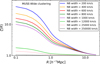 |
Fig. 3. Clustering enhancement factor as a function of comoving transverse separation between LAE pairs. Each color corresponds to a different (FWHM) pseudo-NB width. For reference, we include typical NB widths of 12 000 and 25 000 km s−1 (or 50 and 100 Å) and a broad-band filter width of 250 000 km s−1 (or 1000 Å). We assume that both resolved and undetected sources tend to cluster similarly to the MUSE-Wide LAE sample and include RSDs. |
While typical pseudo-NB widths of 200 − 800 km s−1 (or 0.5 − 4 Å) result in substantial enhancement factors of ≈10 − 40 at R = 0.1 h−1 Mpc, the effective SB values measured with common NB filters FWHM ≈ 50 − 100 Å or 12 000 − 25 000 km s−1 are enhanced by only ζ(R)≈1.5–2 and thus barely boosted by clustering. Unsurprisingly, measurements through broad-band filters with FWHM ≈ 1000 Å (250 000 km s−1) remain entirely unaffected (ζ(R)≈1). Thus, only for the narrow bandwidths achieved by IFU-based Lyα images is there a significant contribution of clustered LAEs to any underlying truly diffuse Lyα emission.
Unless explicitly specified, in the following we fix the bandwidth to ZNB = 3 h−1 Mpc (intermediate FWHM of Z = 6 h−1 Mpc or 600 km s−1: see Sect. 2), corresponding to a window spanning 2.5 Å in the rest frame around λLyα ≈ 1216 Å.
We also have to make assumptions about the clustering behaviour of the undetected sources to calculate the corresponding enhancement factor. Because the FoG effect is negligible at Z > 5 h−1 Mpc (see Fig. 2), we did not include RSDs in the HOD modeling. The modeling process is described below.
As a first step, we assumed that detected and undetected LAEs present the same clustering properties. We show the corresponding boost factor in red in Fig. 4 (same as the red curve in Fig. 3 but without including RSDs; see the negligible difference between the two curves). However, this is likely to be an overestimate: as demonstrated in HA23, the clustering strength depends significantly on Lyα luminosity (8σ in HA23) and, therefore, the even fainter undetected sources probably cluster less strongly than the MUSE-Wide LAEs. Since the enhancement factor depends directly on the clustering strength, this option only produces an upper limit on ζ(R).
 |
Fig. 4. As in Fig. 3 but for a fixed (FWHM) pseudo-NB width of 600 km s−1 and for different assumed clustering strengths for undetected sources, depending on their Lyα luminosity. The red and blue enhancement factors assume that undetected LAEs cluster similarly to MUSE-Wide and MXDF LAEs, respectively. The orange, gray, and green factors assume an extrapolated HOD 2pcf for LAEs with log(LLyα/[erg s−1]) ≈ 40.0, log(LLyα/[erg s−1]) ≈ 38.5, and log(LLyα/[erg s−1]) ≈ 37.0, respectively. In all cases, detected LAEs cluster similarly to what is seen for the MUSE-Wide sample. |
Next, we modified the assumptions and allowed the undetected sources to have a clustering strength similar to the fainter LAEs detected at 3 < z < 5 in the MXDF (HA23), which are approximately one order of magnitude less luminous than the MUSE-Wide sample. As shown in Appendix A for MUSE-Wide, the HOD model derived in HA23 for 3 < z < 6 is also able to describe the clustering of the current MXDF dataset. The resulting boost factor is shown in blue in Fig. 4. Although it is fainter than MUSE-Wide LAEs, the MXDF LAEs are still considerably more luminous than the hidden undetected ones. Hence, this boost factor is also an upper limit.
Finally, to obtain our best estimate of the actual enhancement factor of the undetected LAEs, we utilize the MUSE-Wide and MXDF HOD clustering probability contours of Sect. 4 of HA23 and extrapolate them to fainter luminosities. We first assumed that undetected LAEs have luminosities of log LLyα ≈ 1040 erg s−1 and obtained a HOD model with log(Mmin/[h−1 M⊙]) = 9.9, log(M1/Mmin) = 1.1 and α = 0.1. We plot the resulting boost factor in orange in Fig. 4. We followed the same procedure for the other two lower integration limits (the resulting HOD models have log(Mmin/[h−1 M⊙]) = 9.4, log(M1/Mmin) = 0.7, α = −1.6, and log(Mmin/[h−1 M⊙]) = 8.8, log(M1/Mmin) = 0.3, α = −3.3, respectively), plotting their enhancement factors in gray and green. While the three last enhancement factors are based on extrapolations thereby unstestable at present, we presume that these are probably closer to the truth than the one resulting from the assumption that faint LAEs cluster in the same way as much more luminous objects.
To build the Lyα SB profiles, we have to extrapolate the CCF models down to R = 0 kpc, since our clustering measurements do not reach the smallest scales of the Lyα SB profiles (R < 30 pkpc). We also convert the comoving radii to physical kpc.
4.3. Lyα surface brightness profile from undetected LAEs
In Fig. 5, we build the expected Lyα SB profile from undetected LAEs with log(Lmin/[erg s−1]) = 38.5 for a velocity width of the pseudo-NB of 600 km s−1. The colors show the clustering scenarios considered in Sect. 4.2. For comparison, we overplot the mean Lyα SB profile based on the stacking of LAEs in the MUSE Deep Fields (Sect. 2). We also indicate the typical virial radius of MUSE-Wide LAEs for guidance.
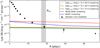 |
Fig. 5. Contribution to the Lyα SB profiles from clustered and undetected LAEs with log(Lmin/[erg s−1]) = 38.5. Differently colored lines correspond to a different assumption for the clustering of undetected LAEs. Detected galaxies are assumed to cluster like those in the MUSE-Wide sample. The data points correspond to the modified stacking experiment of individual LAEs of Wisotzki et al. (2018; see Sects. 2 and 4.4). The triangle denotes an upper limit. We employ a pseudo-NB width of 600 km s−1 and the Lyα LF of Herenz et al. (2019). The shaded gray region shows the typical virial radius of MUSE-Wide LAEs. |
Before comparing the observed profile with the expected contribution from clustered faint LAEs (see Sect. 4.4 below), we have to evaluate the uncertainties and dependencies of our calculations with respect to the assumed input parameters.
We start by considering the different adopted clustering scenarios. By design, the maximum contribution is reached for the MUSE-Wide clustering assumption (≈2.5 × 10⁻²⁰ cgs), whereas the lowest extrapolated HOD model delivers SB levels lower by one order of magnitude (≈4 × 10⁻²¹ cgs). Nevertheless, all versions of our estimates exceed the measurements at R > 60 kpc.
The impact of using different lower integration limits for the LF is evaluated in Fig. 6. Here we assume that the clustering of faint LAEs follows the extrapolated HOD model for log(Lmin/[erg s−1]) = 38.5 LAEs. The three curves show the variation in the SB contribution for various Lmin choices. As expected, the inclusion of fainter sources produces higher Lyα SB levels, although the difference is only a factor of ∼2 for the adopted range of Lmin.
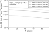 |
Fig. 6. Lyα SB variation for plausible luminosities of the undetected LAEs. We assume that undetected sources cluster like the extrapolated HOD model for log(Lmin/[erg s−1]) = 38.5. Resolved sources cluster like those in the MUSE-Wide sample and the pseudo-NB width is 600 km s−1. We use the Lyα LF from Herenz et al. (2019). |
In Fig. 7, we vary the value of the faint-end LF slope αLF in steps of Δα = ±0.1, recomputing the SB profiles each time. The changes are substantial and demonstrate that the biggest single uncertainty in this estimate is still the faint-end shape of the Lyα LF. We also explored modifying the other LF parameters ϕ* and L*, but these have a negligible effect on the predicted Lyα SB profiles.
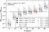 |
Fig. 7. SB ratio of the Lyα SB profile from undetected LAEs and the redone stacked profile from Wisotzki et al. (2018) at 3 < z < 5. The ratios at R = 90 pkpc are lower limits. Undetected LAEs are assumed to cluster like the extrapolated HOD model for Lmin = 1038.5 erg s−1 and resolved sources like those in the MUSE-Wide sample. The colors represent different minimum Lyα luminosities for the undetected sources. The symbols display various faint-end slopes of the Lyα LF. The dashed line shows a scenario in which the undetected LAEs alone fully explain the apparent Lyα SB profile. A pseudo-NB width of 600 km s−1 is assumed. |
4.4. Comparison with observed surface brightness profile
It is clear from Fig. 5 that at R ≲ 20 pkpc the stacked Lyα SB is much higher than the level expected from undetected LAEs, irrespective of the clustering scenario, whereas for radii of ≳50 pkpc, the observed SB level is always comparable to or lower than the contribution estimated from clustering. We note that even where the data points are formally below our calculations, for instance, R = 90 kpc, the combination of error bars in the data with systematic uncertainties in the clustering and luminosity function evaluation imply that these two are not in contradiction.
When interpreting Fig. 5, we have to keep in mind that the two upper (red and blue) curves are upper limits in the sense that for these curves, the clustering of the undetected LAEs is assumed to be as strong as for (different sets of) detected LAEs. Allowing for a weaker clustering of the undetected objects shifts the radius of approximate equality outwards to at least ≈40 pkpc.
Figure 7 shows the inferred SB ratios (clustering/observed) instead of measured or calculated SB levels. For the fiducial baseline faint-end LF slope of αLF = −1.84, the Lyα emission from undetected LAEs can account for all of the measured Lyα SB profile at R ≳ 50 pkpc, but only a fraction of 20% at R ∼ 30 pkpc. At these smaller distances to the central galaxy we presumably see genuine diffuse emission, powered by the above mentioned mechanisms.
These fractions (and the associated radii) are contingent on the uncertainties in the Lyα LF, especially its faint-end, which we here encapsulate by two parameters, the slope αLF, and the low-luminosity cutoff of Lmin. The effects of modifying any of these two are displayed in Fig. 7 by varying the symbols (αLF) and colors (Lmin). It is evident that varying Lmin has a much weaker effect than adopting a different LF slope. An only slightly shallower LF would reduce the expected SB contribution of faint LAEs drastically to ≈20 − 40% at R ∼ 50 pkpc, whereas a steeper slope would imply that extended Lyα emission could be dominated by discrete objects already from distances of 20 − 30 pkpc outwards. It is worth mentioning that if undetected LAEs cluster similarly to the extrapolated HOD models, the minimum luminosity choices of log(Lmin/[erg s−1]) = 37, 40 deliver indistinguishable SB ratios as those of Fig. 7. If undetected LAEs cluster like the LAEs in MUSE-Wide or MXDF, these ratios increase by (on average) ≈70% and ≈30%, respectively. In Appendix C, we show how the SB ratio varies for different pseudo-NB widths.
These are very rough estimates. A sharp cut of the Lyα LF below a certain Lyα luminosity is, of course, implausible. A more realistic shape would probably involve some smooth turnover towards fainter luminosities. Such subtleties are however beyond the scope of this paper. Clearly more work is needed to study the faint parts of the Lyα luminosity function and its possible (non-)evolution with redshift. Nevertheless, our findings strongly support a scenario in which discrete but individually undetected LAEs are an important component of observed Lyα halos at R ≳ 30 − 50 pkpc.
4.5. Comparison with the simulations
Our results are in good agreement with the fundamental prediction from a number of simulation or modeling studies positing that faint LAEs in the vicinity of Lyα halos contribute to the observed extended emission and beyond some radii, they may even dominate (e.g., Lake et al. 2015; Mas-Ribas & Dijkstra 2016; Mas-Ribas et al. 2017; Mitchell et al. 2021; Byrohl et al. 2021). Nevertheless, the models and also the predicted Lyα SB profiles due to “satellite” LAEs vary significantly between different studies. It is also worth mentioning that some of our undetected LAEs are, in principle, at the DMH center.
In the following we compare our Lyα SB profiles calculated from clustering with simulation studies that separate the satellite SB contribution from other powering mechanisms. We give the main differences below.
First, we consider the study of Lake et al. (2015, hereafter L15), where an adaptive mesh refinement hydrodynamical simulation of galaxy formation was used (Bryan & Norman 2000; Joung et al. 2009). These authors modeled most potential sources of Lyα photons and powering mechanisms namely, star formation from central and satellite galaxies, photon scattering, fluorescence from the UV background, supernova feedback (outflows), and gravitational cooling at zsimul = 3.1. The Lyα emission was modeled using the Monte Carlo radiative transfer code of Zheng & Miralda-Escudé (2002). The dark matter particle mass is 1.3 × 10⁷ M⊙, the simulation box size is 120 h−1 Mpc, and the spatial resolution ≈111 pc. Although the derived total Lyα SB profiles match those measured in Matsuda et al. (2012), Xue et al. (2017) found that the simulated profile that included star formation from satellites considerably overpredicted the measured SB curves. To extract the SB profile, they employed a projection depth of 224 pkpc to include all scattered photons around the LAEs.
Next, Mitchell et al. (2021, hereafter M21), employed an adaptive mesh refinement zoom-in cosmological radiation hydrodynamics simulation of a single galaxy using the RAMSES-RT code (Rosdahl et al. 2013; Rosdahl & Teyssier 2015). The stellar and DMH masses are M⋆ = 109.5 M⊙ and Mh = 1011.1 M⊙, respectively. These authors modeled the same Lyα powering mechanisms at 3 < z < 4 as L15. They also performed Monte Carlo radiative transfer to assess the Lyα emission, tracing the emergent radiation along several different lines of sight and at different cosmic times. The simulation box is a sphere of 150 kpc radius and achieved a spatial resolution of 14 pc, with a characteristic dark matter particle mass of 104 M⊙. The simulated total Lyα SB profile matched the one measured in Wisotzki et al. (2018), for which they used a projection depth of ±150 pkpc at zsimul = 3.5 around the LAE.
Finally, Byrohl et al. (2021, hereafter B21), utilized the outcome of the TNG50 (Nelson et al. 2019; Pillepich et al. 2019) from the IllustrisTNG simulations (Pillepich et al. 2018), coupled to their Lyα full radiative transfer code VOROILTIS. They modeled the same Lyα emission sources and powering mechanisms at 2 < z < 5 as L15 and M21 and further included a treatment for active galactic nuclei. TNG50 has a box size of 50 Mpc, attains a spatial resolution of ∼100 pc and a dark matter particle mass of 4.5 × 10⁵ M⊙. These authors were able to reproduce the Lyα SB profiles measured in Leclercq et al. (2017), for which they included all scattered photons from within ±100 pkpc along the line of sight at zsimul = 3 around the LAE.
Although most simulations deliver similar conclusions and their total Lyα SB profiles match a range of observations, the predicted contribution from satellites to the observed radial profiles at various scales varies significantly. We compare in Fig. 8 our clustering-based Lyα SB profiles (with log(Lmin/[erg s−1]) = 38.5, but considering all clustering scenarios) to simulated satellite radial profiles. For this purpose, we recalculate our enhancement factors and SB profiles in order to approximately match our selected pseudo-NB width (i.e., ZNB in Eq. (4)) to the projection depth applied in the simulations. We note that while the pseudo-NB width in observed spectral stacks cannot be narrower than the common linewidth, the typical bandwidths formally converted to real space depths are much greater than simulation boxes. To enable at least a rough comparison we used the simulated depths, which correspond to velocity intervals of ≈60 − 100 km s−1. We also multiplied the simulated profiles by (1 + zsimul)4/(1 + ⟨z⟩)4 to account for surface brightness dimming. The simulated contribution is due to the Lyα emission from satellites in L15 (dashed magenta) and M21 (dashed light blue), and to this plus a genuinely diffuse emission powered by these “other halos” in B21 (dashed light gray).
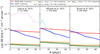 |
Fig. 8. Comparison of our Lyα SB profiles from undetected LAEs of log(Lmin/[erg s−1]) = 38.5 (solid lines) and the satellite radial profiles predicted from simulations (dashed lines). The different colors of the solid curves correspond to the different clustering assumptions for the undetected LAEs displayed in the legend. Resolved LAEs are assumed to cluster in the same way as those in the MUSE-Wide sample. We adjusted our pseudo-NB width of Eq. (4) to the projection depth of the simulations. Left panel: comparison to L15, whose applied projection depth is equivalent to a pseudo-NB width of 66 km s−1 at zsimul = 3.1. Middle panel: comparison to M21 with a pseudo-NB width of 94 km s−1 at zsimul = 3.5. Right panel: comparison to B21 with a pseudo-NB width of 56 km s−1 at zsimul = 3. |
The profile from L15 is clearly flatter than those from M21 and B21 and is in this respect similar to our clustering-based SB profiles. This also agrees with the generally observed trend that the radial profiles tend to flatten at larger radii (Matsuda et al. 2012; Momose et al. 2014; Wisotzki et al. 2018; Niemeyer et al. 2022). On the other hand, the SB level predicted by L15 is much higher than ours, already by an order of magnitude than our two upper limit scenarios. The SB levels predicted by M21 and B21 are in better agreement with our upper limit SB estimates, although still higher than our extrapolated “low clustering” scenarios. This may reflect the fact that simulated galaxies in L15 present higher stellar and DMH masses (M⋆ = 2.9 × 10¹⁰ M⊙ and Mh = 1011.5 M⊙) than those of MUSE LAEs or those considered in M21 and B21. At small scales, the M21 and B21 simulated radial profiles are slightly steeper than the high clustering scenario curves of MUSE-Wide and MXDF.
The differences between our clustering-based and the simulated SB profiles could be attributed to several factors. An overprediction of the simulated number of satellites would naturally lead to an overestimated contribution of discrete LAEs to the Lyα halos. This issue seems to be common to simulations and semi-analytical models, including the IllustrisTNG project and EAGLE simulations (e.g., Okamoto et al. 2010; Simha et al. 2012; Geha et al. 2017; Shuntov et al. 2022). In this context it is interesting to note that our upper limit clustering scenarios give results closer to the simulations than the extrapolations deemed to be more realistic.
Alternatively, there could also be a problem related to low number statistics, since the models by M21 and L15 are based on only one and nine galaxies, respectively. This is probably not an issue for B21, as they did not account for Lyα destruction by dust, which would otherwise lead to overestimated luminosities, and possibly influence the resulting LAH shapes as well. Finally, it is certainly possible that the differences may be partially driven by our assumptions. Our estimated fraction of undetected LAEs might be lower than the actual one, either because of a steeper luminosity function or because of a lower faint-end cutoff.
4.6. How to measure the faint LAE SB contribution
While it seems safe to state that a significant contribution of faint LAEs to the apparent Lyα SB profiles must be expected, at least in qualitative agreement between our empirical framework and the predictions by cosmological simulations, it would be very desirable to further constrain their contribution directly from observations. Here, we embark on a few (partly speculative) considerations of how that might be achieved in the future.
One avenue of investigation could be a comparison between the behaviour of individual and stacked Lyα SB maps at large scales. In principle, this should contain essential information about the faint LAE SB contribution: Stacking at random angles invariably contains some degree of azimuthal averaging which smears out the contributions of individual neighboring LAEs, while individual LAEs have neighbors only in certain directions. Using the deepest existing data, it might be possible to estimate the incidence of clear asymmetries or other external disturbances in individual Lyα halos and use this to constrain the frequency of marginally detectable close neighbours.
Another approach could be to compare the outcomes of different stacking methods, since these differ in terms of the sensitivity to asymmetries in the outskirts: a profile derived from a median-stack of Lyα images should show a different contribution from faint external LAEs than a profile obtained as the mean of several azimuthally averaged individual profiles.
What is also relevant is the bandwidth chosen to extract the LAE pseudo-NB images from the original IFU data, as this influences the contrast between the “background” contribution of unrelated and (with respect to the central galaxy) unclustered LAEs as well as the enhancement due to physical neighbor LAEs at similar redshifts. Varying this bandwidth will provide insights about the relative balance between these two.
Observations seem to show that on average, LAH profiles are remarkably self-similar over a wide range of Lyα luminosities. However, if at some radius the contribution from external LAEs prevails, then the self-similarity should break down around that radius, and profiles obtained at different luminosity levels should converge towards the same behaviour.
At fixed limiting sensitivity, the contribution of faint LAEs to the combined LAH profiles should also decrease rapidly with redshift, simply because of (1 + z)4 dimming together with a (roughly) unevolving luminosity function. While Leclercq et al. (2017) did not find any significant Lyα halo size evolution with redshift, their sizes clearly refer to the “inner” LAHs and leave the outer regions still unconstrained. A slightly stronger boundary condition is the similarity of stacked Lyα profiles at z ≈ 3.5, 4.5, and 5.5 in Wisotzki et al. (2018), which could suggest that at least at high redshifts there is indeed a genuinely diffuse component also in outer regions of LAHs. On the other hand, the same phenomenon could arise from a steepening Lyα LF, and/or an increasing clustering strength of LAEs towards higher redshifts, which would then counteract the cosmological dimming.
We can evaluate whether this scenario is actually realistic. We note that while in Ouchi et al. (2017), HA21, and HA23 no significant clustering dependence on redshift was found, Durkalec et al. (2014) and Khostovan et al. (2019) found a clear increase of clustering strength with cosmic time. To calculate the increase of clustering strength needed to counteract the SB dimming (i.e., (1 + z)−4) in redshift bins of Δz = 1, we would need a factor ≈1.25 increase in the large-scale bias factor, from b ≈ 2.65 for 3 < z < 4 to b ≈ 3.30 for 4 < z < 5 and b ≈ 4.15 for 5 < z < 6. These values are in broad agreement with the clustering growth found in Durkalec et al. (2014) and Khostovan et al. (2019).
Ultimately, building on these suggested analyses and experiments will require more and better data than currently available. Large LAE samples such as that from the Hobby-Eberly Telescope Dark Energy Experiment (HETDEX; Gebhardt et al. 2021) or future LAE integral field spectrographs such as BlueMUSE (Richard et al. 2019) may deliver the data quantity and quality to discern between genuinely diffuse Lyα emission in the circum- and intergalactic medium, on the one hand, and “fake diffuse” contributions from faint undetected LAEs, on the other hand.
5. Conclusions
In this paper, we turn the observed clustering properties of a sample of 1265 Lyα emitting galaxies (LAEs) at 3 < z < 5 from the MUSE-Wide survey into implications for the spatially extended Lyα emission in the circumgalactic medium (CGM) of LAEs. All sources have spectroscopic redshifts and their median Lyα luminosity is log(LLyα/[erg s−1]) ≈ 42.27.
We used halo occupation distribution (HOD) modeling to represent the clustering of our LAE set. Because the extended Lyα emission around LAEs is commonly measured using (pseudo-)narrow-band (NB) filters centered on the Lyα wavelength, we included redshift-space distortions both at large (Kaiser infall) and small (Finger of God effect) scales.
We then extrapolated the HOD statistics inwards towards smaller radii and combined them with assumptions about the Lyα emitter luminosity function (LF). We only considered the emission from undetected LAEs, which are less luminous than the ones in our current dataset. Together, these two ingredients are transformed into a (upper-limit) Lyα surface brightness (SB) profile, which belongs to individually undetected close neighbors that cluster like those in the MUSE-Wide sample. We derived a maximum SB values of SB ≈ 2.5 × 10⁻²⁰ erg s−1 cm−2 arcsec−2, assuming a luminosity of the undetected LAEs of log(LLyα/[erg s−1]) = 38.5.
We considered various alternative clustering scenarios for the undetected sources. We first assumed that these follow the same clustering properties as the LAEs in the MUSE-Extremely Deep Field (MXDF; one order of magnitude fainter than those in MUSE-Wide but still more luminous than undetected LAEs) and compute the corresponding (upper limit) radial profile (SB ≈ 2 × 10⁻²⁰ cgs). We then extrapolated the clustering properties of MUSE-Wide and MXDF LAEs down to log(LLyα/[erg s−1]) ≈ 37.0, 38.5, 40.0 and used the resulting HOD models to estimate the actual Lyα SB profiles from undetected LAEs. We obtained a maximum SB of SB ≈ 4 × 10⁻²¹ cgs.
We compared our log(LLyα/[erg s−1]) = 38.5 undetected Lyα SB profile to the LAE stacking experiment performed in Wisotzki et al. (2018) to address the question of whether undetected LAEs play a pivotal role in the formation of the extended Lyα halos. Assuming a simple Schechter LF with a reasonable intermediate faint-end slope (−1.94 ≤ αLF ≤ −1.84) and a lower limit for Lyα luminosities of the undetected LAEs (log(LLyα/[erg s−1]) ≈ 38.5), we find that the stellar irradiation from those undetected LAEs can dominate the excess surface brightness at large scales (R ≳ 50 pkpc). On the other hand, the Lyα SB profile at small scales (R ≲ 20 pkpc) cannot be explained by undetected sources and may be better explained by a genuinely diffuse origin. More luminous LAEs (log(LLyα/[erg s−1]) ≈ 40) reproduce at best 4%, 40%, and 100% of the extended emission at R = 15, 40, 65 pkpc, respectively.
We also compared our estimated Lyα SB profiles with simulation studies. Although we agree that faint LAEs dominate the SB of the Lyα halos at large scales, the shape of the radial profiles and the contribution to the total Lyα SB profiles differ. While the simulated faint LAE SB profiles generally decrease rapidly with distance, our derived radial profiles have shallow slopes, likely leading to the flattening at R ≳ 30 pkpc seen in observed Lyα SB profiles Overall, most simulated profiles, together with our estimations, infer a faint LAE contribution of the same order of magnitude.
Although these faint LAEs are likely the most significant source of luminosity for the outer parts of observed Lyα halos, beyond the scales probed by most observations of single objects (R > 50 pkpc), the actual point at which this contribution starts to become important depends crucially on the shape of the Lyα luminosity function, in particular, its faint end. We also suggest a few experiments to directly constrain the faint LAE SB contribution from observations.
Acknowledgments
The authors give thanks to the staff at ESO for extensive support during the visitor-mode campaigns at Paranal Observatory. We thank the eScience group at AIP for help with the functionality of the MUSE-Wide data release webpage. T.M. thanks for financial support by CONACyT Grant Científica Básica #252531 and by UNAM-DGAPA (PASPA, PAPIIT IN111319 and IN114423). L.W. and J.P. by the Deutsche Forschungsgemeinschaft through grant Wi 1369/31-1. The data were obtained with the European Southern Observatory Very Large Telescope, Paranal, Chile, under Large Program 1101.A-0127. This research made use of Astropy, a community-developed core Python package for Astronomy (Astropy Collaboration 2013). We also thank the referee for an useful and constructive report.
References
- Adelberger, K. L., Steidel, C. C., Pettini, M., et al. 2005, ApJ, 619, 697 [NASA ADS] [CrossRef] [Google Scholar]
- Astropy Collaboration (Adelberger, K. L., et al.) 2013, A&A, 558, A33 [NASA ADS] [CrossRef] [EDP Sciences] [Google Scholar]
- Bacon, R., Accardo, M., Adjali, L., et al. 2010, SPIE, 7735, 131 [Google Scholar]
- Bacon, R., Brinchmann, J., Richard, J., et al. 2015, A&A, 575, A75 [NASA ADS] [CrossRef] [EDP Sciences] [Google Scholar]
- Bacon, R., Conseil, D., Mary, D., et al. 2017, A&A, 608, A1 [NASA ADS] [CrossRef] [EDP Sciences] [Google Scholar]
- Bacon, R., Mary, D., Garel, T., et al. 2021, A&A, 647, A107 [NASA ADS] [CrossRef] [EDP Sciences] [Google Scholar]
- Bacon, R., Brinchmann, J., Conseil, S., et al. 2022, A&A, 670, A4 [Google Scholar]
- Bahcall, J. N., & Spitzer, L., Jr 1969, ApJ, 156, L63 [NASA ADS] [CrossRef] [Google Scholar]
- Bryan, G. L., & Norman, M. L. 2000, IMA, 117, 165 [NASA ADS] [Google Scholar]
- Byrohl, C., Nelson, D., Behrens, C., et al. 2021, MNRAS, 506, 5129 [NASA ADS] [CrossRef] [Google Scholar]
- Claeyssens, A., Richard, J., Blaizot, J., et al. 2022, A&A, 666, A78 [NASA ADS] [CrossRef] [EDP Sciences] [Google Scholar]
- de La Vieuville, G., Bina, D., Pello, R., et al. 2019, A&A, 628, A3 [NASA ADS] [CrossRef] [EDP Sciences] [Google Scholar]
- Dijkstra, M., & Kramer, R. 2012, MNRAS, 424, 1672 [NASA ADS] [CrossRef] [Google Scholar]
- Drake, A. B., Garel, T., Wisotzki, L., et al. 2017, A&A, 608, A6 [NASA ADS] [CrossRef] [EDP Sciences] [Google Scholar]
- Durkalec, A., Le Fèvre, O., Pollo, A., et al. 2014, A&A, 583, A128 [Google Scholar]
- Finkelstein, S. L., Cohen, S. H., Windhorst, R. A., et al. 2011, ApJ, 735, 5 [NASA ADS] [CrossRef] [Google Scholar]
- Garel, T., Blaizot, J., Guiderdoni, B., et al. 2015, MNRAS, 450, 1279 [Google Scholar]
- Gebhardt, K., Cooper, E. M., Ciardullo, R., et al. 2021, ApJ, 923, 217 [NASA ADS] [CrossRef] [Google Scholar]
- Geha, M., Wechsler, R. H., Mao, Y., et al. 2017, ApJ, 847, 4 [NASA ADS] [CrossRef] [Google Scholar]
- Gronke, M., & Bird, S. 2017, ApJ, 835, 207 [NASA ADS] [CrossRef] [Google Scholar]
- Hashimoto, T., Verhamme, A., Ouchi, M., et al. 2015, ApJ, 812, 157 [Google Scholar]
- Hayashino, T., Matsuda, Y., Tamura, H., et al. 2004, AJ, 128, 2073 [Google Scholar]
- Herenz, E. C., Urrutia, T., Wisotzki, L., et al. 2017, A&A, 606, A12 [NASA ADS] [CrossRef] [EDP Sciences] [Google Scholar]
- Herenz, E. C., Wisotzki, L., Saust, R., et al. 2019, A&A, 621, A107 [NASA ADS] [CrossRef] [EDP Sciences] [Google Scholar]
- Herrero Alonso, Y., Krumpe, M., Wisotzki, L., et al. 2021, A&A, 653, A136 [NASA ADS] [CrossRef] [EDP Sciences] [Google Scholar]
- Herrero Alonso, Y., Miyaji, T., Wisotzki, L., et al. 2023, A&A, 671, A5 [NASA ADS] [CrossRef] [EDP Sciences] [Google Scholar]
- Hinshaw, G., Larson, D., Komatsu, E., et al. 2013, ApJS, 208, 19 [Google Scholar]
- Joung, M. R., Cen, R., & Bryan, G. L. 2009, ApJ, 692, L1 [NASA ADS] [CrossRef] [Google Scholar]
- Kaiser, N. 1987, MNRAS, 227, 1 [Google Scholar]
- Kakiichi, K., & Dijkstra, M. 2018, MNRAS, 4, 5140 [NASA ADS] [Google Scholar]
- Kennicutt, R. C., Jr. 1998, ApJ, 498, 541 [Google Scholar]
- Khostovan, A. A., Sobral, D., Mobasher, B., et al. 2019, MNRAS, 489, 555 [Google Scholar]
- Konno, A., Ouchi, M., Shibuya, T., et al. 2018, PASJ, 70, S16 [Google Scholar]
- Kusakabe, H., Verhamme, A., Blaizot, J., et al. 2022, A&A, 660, A44 [NASA ADS] [CrossRef] [EDP Sciences] [Google Scholar]
- Lake, E., Zheng, Z., Cen, R., et al. 2015, ApJ, 806, 46 [NASA ADS] [CrossRef] [Google Scholar]
- Leclercq, F., Bacon, R., Wisotzki, L., et al. 2017, A&A, 608, A8 [NASA ADS] [CrossRef] [EDP Sciences] [Google Scholar]
- Mas-Ribas, L., & Dijkstra, M. 2016, ApJ, 822, 84 [Google Scholar]
- Mas-Ribas, L., Dijkstra, M., Hennawi, J. F., et al. 2017, ApJ, 841, 19 [Google Scholar]
- Matsuda, Y., Yamada, T., Hayashino, T., et al. 2012, MNRAS, 425, 878 [NASA ADS] [CrossRef] [Google Scholar]
- Mitchell, P., Blaizot, J., Cadiou, C., & Dubois, Y. 2021, MNRAS, 501, 5757 [Google Scholar]
- Momose, R., Ouchi, M., Nakajima, K., et al. 2014, MNRAS, 442, 110 [NASA ADS] [CrossRef] [Google Scholar]
- Momose, R., Ouchi, M., Nakajima, K., et al. 2016, MNRAS, 457, 2318 [NASA ADS] [CrossRef] [Google Scholar]
- Muzahid, S., Schaye, J., Marino, R. A., et al. 2020, MNRAS, 496, 1013 [Google Scholar]
- Nelson, D., Pillepich, A., Springel, V., et al. 2019, MNRAS, 490, 3234 [Google Scholar]
- Niemeyer, M. L., Komatsu, E., Byrohl, C., et al. 2022, ApJ, 929, 90 [NASA ADS] [CrossRef] [Google Scholar]
- Nilsson, K. K., Tapken, C., Müller, P., et al. 2009, A&A, 498, 13 [NASA ADS] [CrossRef] [EDP Sciences] [Google Scholar]
- Okamoto, T., Frenk, C. S., Jenkins, A., et al. 2010, MNRAS, 406, 208 [NASA ADS] [CrossRef] [Google Scholar]
- Ouchi, M., Shimasaku, K., Akiyama, M., et al. 2008, ApJS, 176, 301 [Google Scholar]
- Ouchi, M., Harikane, Y., Shibuya, T., et al. 2017, PASJ, 70, S13 [NASA ADS] [Google Scholar]
- Partridge, R. B., & Peebles, P. J. E. 1967, ApJ, 147, 868 [Google Scholar]
- Peebles, P. J. E. 1980, Large-Scale Structure of the Universe (Princeton: Princeton University Press), 196, 435 [Google Scholar]
- Pillepich, A., Springel, V., Nelson, D., et al. 2018, MNRAS, 475, 648 [NASA ADS] [CrossRef] [Google Scholar]
- Pillepich, A., Nelson, D., Springel, V., et al. 2019, MNRAS, 490, 3196 [Google Scholar]
- Richard, J., Bacon, R., Blaizot, J., et al. 2019, ArXiv e-prints [arXiv:1906.01657] [Google Scholar]
- Rosdahl, J., & Teyssier, R. 2015, MNRAS, 449, 4380 [Google Scholar]
- Rosdahl, J., Blaizot, J., Aubert, D., et al. 2013, MNRAS, 436, 2188 [NASA ADS] [CrossRef] [Google Scholar]
- Schechter, P. 1976, ApJ, 203, 297 [Google Scholar]
- Schmidt, B. K., Kerutt, J., Wisotzki, L., et al. 2021, A&A, 654, A80 [NASA ADS] [CrossRef] [EDP Sciences] [Google Scholar]
- Shimizu, I., & Umemura, M. 2010, MNRAS, 406, 913 [NASA ADS] [Google Scholar]
- Shuntov, M., McCracken, H. J., Gavazzi, R., et al. 2022, A&A, 664, A61 [NASA ADS] [CrossRef] [EDP Sciences] [Google Scholar]
- Simha, V., Weinber, D. H., Davé, R., et al. 2012, MNRAS, 423, 3458 [NASA ADS] [CrossRef] [Google Scholar]
- Sobral, D., Santos, S., Matthee, J., et al. 2018, MNRAS, 476, 4725 [Google Scholar]
- Steidel, C. C., Bogosavljevic, M., Shapley, A. E., et al. 2011, ApJ, 736, 160 [NASA ADS] [CrossRef] [Google Scholar]
- Tinker, J. L. 2007, MNRAS, 374, 477 [NASA ADS] [CrossRef] [Google Scholar]
- Urrutia, T., Wisotzki, L., Kerutt, J., et al. 2019, A&A, 624, A141 [NASA ADS] [CrossRef] [EDP Sciences] [Google Scholar]
- van den Bosch, F. C., More, S., Cacciato, M., et al. 2013, MNRAS, 430, 725 [NASA ADS] [CrossRef] [Google Scholar]
- Verhamme, A., Garel, T., Ventou, E., et al. 2018, MNRAS, 478, 60 [Google Scholar]
- Wisotzki, L., Bacon, R., Blaizot, J., et al. 2016, A&A, 587, A98 [NASA ADS] [CrossRef] [EDP Sciences] [Google Scholar]
- Wisotzki, L., Bacon, R., Brinchmann, J., et al. 2018, Nature, 562, 229 [Google Scholar]
- Xue, R., Lee, K. S., Dey, A., et al. 2017, ApJ, 837, 172 [NASA ADS] [CrossRef] [Google Scholar]
- Zhang, H., Cai, Z., Liang, Y., et al. 2023, ArXiv e-prints [arXiv:2301.07358] [Google Scholar]
- Zheng, Z., & Miralda-Escudé, J. 2002, ApJ, 578, 33 [NASA ADS] [CrossRef] [Google Scholar]
- Zheng, Z., Coil, A., & Zehavi, I. 2007, ApJ, 667, 760 [NASA ADS] [CrossRef] [Google Scholar]
- Zheng, Z., Cen, R., Trac, H., & Miralda-Escudé, J. 2011, ApJ, 726, 38 [NASA ADS] [CrossRef] [Google Scholar]
Appendix A: Clustering comparison from LAE subsets of the MUSE-Wide survey
In this work, we utilized the clustering constraints derived in HA23 for a subset of 1030 MUSE-Wide LAEs at 3 < z < 6 to estimate the contribution of undetected LAEs to the apparent Lyα halos observed at 3 < z < 5. To be consistent with the Lyα halo measurements, we focused on a subsample of 1265 LAEs at 3 < z < 5 from the MUSE-Wide survey. In the following, we demonstrate that the LAEs in these two datasets have nearly identical clustering strengths.
In Fig. A.1, we represent in blue the K-estimator measurements obtained in HA23 for the 3 < z < 6 LAE subsample and in red the corresponding measurement for the 3 < z < 5 LAE subset of this work. The clustering strengths are in excellent agreement. The clustering uncertainties for the former sample are (on average) 2% larger than for the latter dataset. The best-fit HOD model and, thus, the large-scale bias factor and typical DMH masses are indistinguishable.
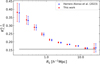 |
Fig. A.1. Clustering strength as measured by the K-estimator (Adelberger et al. 2005) for the LAE dataset considered in HA23 at 3 < z < 6 (blue) and that of the LAE sample at 3 < z < 5 used in this work (red). The black baseline represents the expected value for an unclustered sample. The error bars are Poissonian. The red measurements have been shifted along the x-axis for visual purposes. |
Appendix B: Clustering enhancement factor derivation
The surface brightness (SB) at cosmological distances is defined as
![$$ \begin{aligned} \mathrm{SB} =\int _{Z}\epsilon (Z)\frac{[D_{\rm {A}}(z)(1+z)]^2}{4\pi D_{\rm {L}}(z)^2}\mathrm{d}Z\approx \frac{\epsilon \Delta Z}{4\pi (1+z)^2}, \end{aligned} $$](/articles/aa/full_html/2023/09/aa47294-23/aa47294-23-eq11.gif)
where ϵ(Z) is the comoving volume emissivity as a function of radial comoving separation, Z, and DL, DA = DL/(1 + z)2 are the luminosity and angular size distances at redshift, z, respectively. The radial comoving separation Z corresponds to the (pseudo-)NB width employed to stack LAE images in the measurement of Lyα SB profiles. This definition considers the shape and expansion history of the universe and assumes that objects are randomly distributed.
To account for the clustering of galaxies, we include the excess probability dP of finding a galaxy, i, in a volume element dV at a separation  from another galaxy, j, that is, the two-point correlation function (ξ(R); Peebles 1980)
![$$ \begin{aligned} \mathrm{d}P=n\cdot [1+\xi (R)]\cdot \mathrm{d}V \propto [1+\xi (R)]\cdot \frac{\mathrm{d}Z}{\mathrm{d}z}\mathrm{d}z, \end{aligned} $$](/articles/aa/full_html/2023/09/aa47294-23/aa47294-23-eq13.gif)
where n is the mean number density of the galaxy sample and Rij is the transverse separation between the galaxy pair. The two-point correlation function of interest is, in fact, a cross-correlation function between detected and undetected LAEs. This is because Lyα SB profiles represent SB as function of distance from the central LAE outwards, not as function of observed LAE−observed LAE separation. Hence, the SB that accounts for galaxy clustering is:
![$$ \begin{aligned} \mathrm{SB}&=\int _{Z}\frac{\epsilon (Z)}{4\pi (1+z)^2}\cdot [1+\xi (R)]\cdot \frac{\mathrm{d}Z}{\mathrm{d}z}\mathrm{d}z\approx \nonumber \\&\qquad \qquad \frac{\epsilon }{4\pi (1+z)^2}\int _{Z}[1+\xi (R)]\cdot \mathrm{d}Z. \end{aligned} $$](/articles/aa/full_html/2023/09/aa47294-23/aa47294-23-eq14.gif)
We derive the clustering enhancement factor ζ(R) from the comparison between Eqs. B.1 and B.3 as:
Appendix C: Effect of the velocity bandwidth on the faint LAE contribution to the extended LAHs
To compute the faint LAE SB profiles (colored lines in Fig. 5) and to modify the stacking analysis of Wisotzki et al. (2018) (data points in Fig. 5), we adopted a fixed velocity bandwidth of 600 km s−1. The selected pseudo-NB width influences the Lyα SB values of the stacked radial profile, the background Lyα SB level due to discrete faint LAEs, and the clustering enhancement factor (Eq. 4). The general trend is that, for broader velocity widths, the stacked SB profile notably rises in the outer regions (R > 20 pkpc), the background SB slightly increases, and the clustering enhancement factor significantly declines (see Fig. 3). The interplay between these three factors is thus reflected in the SB ratio of Fig. 7.
In Fig. C.1, we recompute the ratio between the faint LAE SB profile and the stacked one for a pseudo-NB width of 400 km s−1 (left panel) and 800 km s−1 (right panel). For broader bandwidths, the SB ratios decrease because the corresponding decline of the clustering enhancement factor exceeds the smaller rises in the stacked radial profile and the background SB level. While a broadening of the pseudo-NB width from 400 km s−1 to 600 km s−1 causes a maximum 40% drop of the SB ratios, an increase from 600 km s−1 to 800 km s−1 further decreases the SB ratios in at most 20%. We note that for a velocity offset of 600 km s−1 or 800 km s−1, the stacked Lyα SB value at R = 90 pkpc is an upper limit (see e.g., Fig. 5). For 400 km s−1, on the other hand, there is no detection.
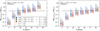 |
Fig. C.1. SB ratio of the Lyα SB profile from undetected LAEs and the modified stacked profile from Wisotzki et al. (2018). Left: Same as Fig. 7 but for a pseudo-NB width of 400 km s−1. Right: Same for a pseudo-NB width of 800 km s−1. |
All Figures
|
Fig. 1. Distribution in Lyα luminosity-redshift space of the 3 < z < 5 LAEs selected from the spectroscopic MUSE-Wide survey. The dashed line corresponds to the median log LLyα of the sample. The normalized redshift and log LLyα distributions are shown in the top and right panels, respectively. |
| In the text | |
|
Fig. 2. Best-fit HOD modeled real- and redshift-space 2pcf. Left: real-space 2pcf, ξ(r), for the sample of MUSE-Wide LAEs at 3 < z < 5. Note: the circular symmetry of the color-coded contours. Right: redshift-space 2pcf, ξ(s). The dotted blue contours show the real-space 2pcf from the left panel. Note: the elongation of the 2pcf contours along the line-of-sight direction, Zs, at small scales (FoG effect) and the flattening at larger transverse separations, R, (Kaiser infall). The contour levels are indicated in the legend. |
| In the text | |
|
Fig. 3. Clustering enhancement factor as a function of comoving transverse separation between LAE pairs. Each color corresponds to a different (FWHM) pseudo-NB width. For reference, we include typical NB widths of 12 000 and 25 000 km s−1 (or 50 and 100 Å) and a broad-band filter width of 250 000 km s−1 (or 1000 Å). We assume that both resolved and undetected sources tend to cluster similarly to the MUSE-Wide LAE sample and include RSDs. |
| In the text | |
|
Fig. 4. As in Fig. 3 but for a fixed (FWHM) pseudo-NB width of 600 km s−1 and for different assumed clustering strengths for undetected sources, depending on their Lyα luminosity. The red and blue enhancement factors assume that undetected LAEs cluster similarly to MUSE-Wide and MXDF LAEs, respectively. The orange, gray, and green factors assume an extrapolated HOD 2pcf for LAEs with log(LLyα/[erg s−1]) ≈ 40.0, log(LLyα/[erg s−1]) ≈ 38.5, and log(LLyα/[erg s−1]) ≈ 37.0, respectively. In all cases, detected LAEs cluster similarly to what is seen for the MUSE-Wide sample. |
| In the text | |
|
Fig. 5. Contribution to the Lyα SB profiles from clustered and undetected LAEs with log(Lmin/[erg s−1]) = 38.5. Differently colored lines correspond to a different assumption for the clustering of undetected LAEs. Detected galaxies are assumed to cluster like those in the MUSE-Wide sample. The data points correspond to the modified stacking experiment of individual LAEs of Wisotzki et al. (2018; see Sects. 2 and 4.4). The triangle denotes an upper limit. We employ a pseudo-NB width of 600 km s−1 and the Lyα LF of Herenz et al. (2019). The shaded gray region shows the typical virial radius of MUSE-Wide LAEs. |
| In the text | |
|
Fig. 6. Lyα SB variation for plausible luminosities of the undetected LAEs. We assume that undetected sources cluster like the extrapolated HOD model for log(Lmin/[erg s−1]) = 38.5. Resolved sources cluster like those in the MUSE-Wide sample and the pseudo-NB width is 600 km s−1. We use the Lyα LF from Herenz et al. (2019). |
| In the text | |
|
Fig. 7. SB ratio of the Lyα SB profile from undetected LAEs and the redone stacked profile from Wisotzki et al. (2018) at 3 < z < 5. The ratios at R = 90 pkpc are lower limits. Undetected LAEs are assumed to cluster like the extrapolated HOD model for Lmin = 1038.5 erg s−1 and resolved sources like those in the MUSE-Wide sample. The colors represent different minimum Lyα luminosities for the undetected sources. The symbols display various faint-end slopes of the Lyα LF. The dashed line shows a scenario in which the undetected LAEs alone fully explain the apparent Lyα SB profile. A pseudo-NB width of 600 km s−1 is assumed. |
| In the text | |
|
Fig. 8. Comparison of our Lyα SB profiles from undetected LAEs of log(Lmin/[erg s−1]) = 38.5 (solid lines) and the satellite radial profiles predicted from simulations (dashed lines). The different colors of the solid curves correspond to the different clustering assumptions for the undetected LAEs displayed in the legend. Resolved LAEs are assumed to cluster in the same way as those in the MUSE-Wide sample. We adjusted our pseudo-NB width of Eq. (4) to the projection depth of the simulations. Left panel: comparison to L15, whose applied projection depth is equivalent to a pseudo-NB width of 66 km s−1 at zsimul = 3.1. Middle panel: comparison to M21 with a pseudo-NB width of 94 km s−1 at zsimul = 3.5. Right panel: comparison to B21 with a pseudo-NB width of 56 km s−1 at zsimul = 3. |
| In the text | |
|
Fig. A.1. Clustering strength as measured by the K-estimator (Adelberger et al. 2005) for the LAE dataset considered in HA23 at 3 < z < 6 (blue) and that of the LAE sample at 3 < z < 5 used in this work (red). The black baseline represents the expected value for an unclustered sample. The error bars are Poissonian. The red measurements have been shifted along the x-axis for visual purposes. |
| In the text | |
|
Fig. C.1. SB ratio of the Lyα SB profile from undetected LAEs and the modified stacked profile from Wisotzki et al. (2018). Left: Same as Fig. 7 but for a pseudo-NB width of 400 km s−1. Right: Same for a pseudo-NB width of 800 km s−1. |
| In the text | |
Current usage metrics show cumulative count of Article Views (full-text article views including HTML views, PDF and ePub downloads, according to the available data) and Abstracts Views on Vision4Press platform.
Data correspond to usage on the plateform after 2015. The current usage metrics is available 48-96 hours after online publication and is updated daily on week days.
Initial download of the metrics may take a while.