| Issue |
A&A
Volume 676, August 2023
|
|
|---|---|---|
| Article Number | A97 | |
| Number of page(s) | 10 | |
| Section | Planets and planetary systems | |
| DOI | https://doi.org/10.1051/0004-6361/202346667 | |
| Published online | 14 August 2023 | |
KMT-2022-BLG-0475Lb and KMT-2022-BLG-1480Lb: Microlensing ice giants detected via the non-caustic-crossing channel
1
Department of Physics, Chungbuk National University,
Cheongju
28644, Republic of Korea
e-mail: cheongho@astroph.chungbuk.ac.kr
2
Korea Astronomy and Space Science Institute,
Daejon
34055, Republic of Korea
3
Institute of Natural and Mathematical Science, Massey University,
Auckland
0745, New Zealand
4
Center for Astrophysics, Harvard & Smithsonian,
60 Garden St.,
Cambridge, MA
02138, USA
5
Department of Astronomy, Tsinghua University,
Beijing
100084, PR China
6
University of Canterbury, Department of Physics and Astronomy,
Private Bag 4800,
Christchurch
8020, New Zealand
7
Max-Planck-Institute for Astronomy,
Königstuhl 17,
69117
Heidelberg, Germany
8
Department of Astronomy, Ohio State University,
140 W. 18th Ave.,
Columbus, OH
43210, USA
9
Korea University of Science and Technology, Korea, (UST),
217 Gajeong-ro, Yuseong-gu,
Daejeon,
34113, Republic of Korea
10
Department of Particle Physics and Astrophysics, Weizmann Institute of Science,
Rehovot
76100, Israel
11
School of Space Research, Kyung Hee University,
Yongin, Kyeonggi
17104, Republic of Korea
12
Institute for Space-Earth Environmental Research, Nagoya University,
Nagoya
464-8601, Japan
13
Code 667, NASA Goddard Space Flight Center,
Greenbelt, MD
20771, USA
14
Department of Astronomy, University of Maryland,
College Park, MD
20742, USA
15
Komaba Institute for Science, The University of Tokyo,
3-8-1 Komaba, Meguro,
Tokyo
153-8902, Japan
16
Instituto de Astrofísica de Canarias,
Vía Láctea s/n,
38205
La Laguna, Tenerife, Spain
17
Department of Earth and Space Science, Graduate School of Science, Osaka University,
Toyonaka, Osaka
560-0043, Japan
18
Department of Physics, The Catholic University of America,
Washington, DC
20064, USA
19
Department of Astronomy, Graduate School of Science, The University of Tokyo,
7-3-1 Hongo, Bunkyo-ku,
Tokyo
113-0033, Japan
20
Sorbonne Université, CNRS, UMR 7095, Institut d’Astrophysique de Paris,
98 bis bd Arago,
75014
Paris, France
21
Department of Physics, University of Auckland,
Private Bag 92019,
Auckland, New Zealand
22
University of Canterbury Mt. John Observatory,
PO Box 56,
Lake Tekapo
8770, New Zealand
Received:
17
April
2023
Accepted:
30
June
2023
Aims. We investigate the microlensing data collected in the 2022 season from high-cadence microlensing surveys in order to find weak signals produced by planetary companions to lenses.
Methods. From these searches, we find that two lensing events, KMT-2022-BLG-0475 and KMT-2022-BLG-1480, exhibit weak short-term anomalies. From a detailed modeling of the lensing light curves, we determine that the anomalies are produced by planetary companions with a mass ratio to the primary of q ~ 1.8 × 10⁻⁴ for KMT-2022-BLG-0475L and q ~ 4.3 × 10⁻⁴ for KMT-2022-BLG-1480L.
Results. We estimate that the host and planet masses and the projected planet-host separation are (Mh/M⊙, Mp/MU, a⊥/au) = (0.43−0.23+0.35, 1.73−0.92+1.42, 2.03−0.38+0.25) for KMT-2022-BLG-0475L and (0.18−0.09+0.16, 1.82−0.92+1.60, 1.22−0.14+0.15) for KMT-2022-BLG-1480L, where MU denotes the mass of Uranus. The two planetary systems have some characteristics in common: the primaries of the lenses are early-mid M dwarfs that lie in the Galactic bulge, and the companions are ice giants that lie beyond the snow lines of the planetary systems.
Key words: planets and satellites: detection / gravitational lensing: micro
© The Authors 2023
 Open Access article, published by EDP Sciences, under the terms of the Creative Commons Attribution License (https://creativecommons.org/licenses/by/4.0), which permits unrestricted use, distribution, and reproduction in any medium, provided the original work is properly cited.
This article is published in open access under the Subscribe to Open model. Subscribe to A&A to support open access publication.
1 Introduction
The microlensing signal of a planet usually appears as a short-term anomaly on the smooth and symmetric lensing light curve generated by the host of the planet (Mao & Paczyński 1991; Gould & Loeb 1992). The signal arises when a source approaches the perturbation region formed around the caustic induced by the planet. Caustics represent the positions on the source plane at which the lensing magnification of a point source is infinite, and thus source crossings over the caustic result in strong signals with characteristic spike features.
The region of planetary deviations extends beyond caustics, and planetary signals can be produced without the caustic crossing of a source. Planetary signals produced via the non-caustic-crossing channel are weaker than those generated by caustic crossings, and the strength of the signal diminishes as the separation of the source from the caustic increases. Furthermore, these signals do not exhibit characteristic features such as the spikes produced by caustic crossings. Due to the combination of these weak and featureless characteristics, the planetary signals generated via the non-caustic channel are difficult to notice. If such signals are missed despite meeting the detection criterion, statistical studies based on the incomplete planet sample would lead to erroneous results on the demographics of planets. To prevent this, the Korea Microlensing Telescope Network (KMTNet; Kim et al. 2016) group regularly conducts a systematic inspection of the data collected by survey experiments, searching for weak planetary signals, and has reported on the detected planets in a series of papers (Zang et al. 2021a,b, 2022, 2023; Hwang et al. 2022; Wang et al. 2022; Gould et al. 2022; Jung et al. 2022, 2023; Han et al. 2022a,b,c,d,e, 2023a; Shin et al. 2023).
In this work, we present analyses of the two microlensing events, KMT-2022-BLG-0475 and KMT-2022-BLG-1480, for which weak short-term anomalies were found from the systematic investigation of the data collected from high-cadence microlensing surveys conducted in the 2022 season. We investigate the nature of the anomalies by carrying out detailed analyses of the light curves.
The organization of the paper is as follows. In Sect. 2, we describe the observations and data used in the analyses. In Sect. 3, we begin by explaining the parameters used in modeling the lensing light curves, and we then detail the analyses conducted for the individual events, KMT-2022-BLG-0475 (Sect. 3.1) and KMT-2022-BLG-1480 (Sect. 3.2). In Sect. 4, we explain the procedure for constraining the source stars and estimating the angular Einstein radii of the events. In Sect. 5, we explain the procedure of the Bayesian analyses conducted to determine the physical lens parameters, and we present the estimated parameters. We summarize our results and conclude in Sect. 6.
2 Observations and data
We inspected the microlensing data of the KMTNet survey collected from observations conducted in the 2022 season. The total number of KMTNet lensing events detected in the season is 2803. For the individual events, we first fitted light curves with a single-lens single-source (1L1S) model and then visually inspected residuals from the model. From this inspection, we found that the lensing events KMT-2022-BLG-0475 and KMT-2022-BLG-1480 exhibited weak short-term anomalies. We then cross-checked whether there were additional data from the surveys conducted by other microlensing observation groups. We find that both events were additionally observed by the Microlensing Observations in Astrophysics (MOA; Bond et al. 2011) group, who referred to them as MOA-2022-BLG-185 and MOA-2022-BLG-383, respectively. For KMT-2022-BLG-1480, there were extra data acquired from the survey observations conducted by the Microlensing Astronomy Probe (MAP) collaboration during the period from 2021 August to 2022 September, whose primary purpose was to verify short-term planetary signals found by the KMTNet survey. In the analyses of the events, we used the combined data from the three survey experiments1.
The observations of the events were carried out using the telescopes that are operated by the individual survey groups. The three identical telescopes used by the KMTNet group have a 1.6 m aperture equipped with a camera yielding 4 deg2 field of view, and they are distributed in the three continents of the Southern Hemisphere for the continuous coverage of lensing events. The sites of the individual KMTNet telescopes are the Cerro Tololo Interamerican Observatory in Chile (KMTC), the South African Astronomical Observatory in South Africa (KMTS), and the Siding Spring Observatory in Australia (KMTA). The MOA group utilizes the 1.8 m telescope at the Mt. John Observatory in New Zealand, and the camera mounted on the telescope has a 1.2 deg2 field of view. The MAP collaboration uses the 3.6 m Canada-France-Hawaii Telescope (CFHT) in Hawaii.
Observations by the KMTNet, MOA, and MAP groups were done mainly in the I, customized MOA-R, and SDSS-i bands, respectively. A fraction of images taken by the KMTNet and MOA surveys were acquired in the V band for the measurement of the source colors of the events. Reduction of data and photometry of source stars were done using the pipelines of the individual survey groups. For the data used in the analyses, we readjusted the error bars estimated from the automated pipelines so that the error bars are consistent with the scatter of data and the χ2 per degree of freedom (dof) for each data set becomes unity, following the method described in Yee et al. (2012).
3 Light curve analyses
The analyses of the lensing events were carried out by searching for lensing solutions specified by the sets of lensing parameters that best describe the observed light curves. The lensing parameters vary depending on the interpretation of an event. It is known that a short-term anomaly can be produced by two channels, in which the first is a binary-lens single-source (2L1S) channel with a low-mass companion to the lens, and the other is a single-lens binary-source (1L2S) channel with a faint companion to the source (Gaudi 1998).
The basic lensing parameters used in common for the 2L1S and 1L2S models are (t0, u0, tE, ρ). The first two parameters represent the time of the closest source approach to the lens and the lens-source separation (impact parameter) scaled to the angular Einstein radius θΕ at t0, respectively. The third parameter denotes the event timescale, which is defined as the time for the source to transit θΕ. The last parameter is the normalized source radius, which is defined as the ratio of the angular source radius θ* to θΕ. The normalized source radius is needed in modeling to describe the deformation of a lensing light curve caused by finite-source effects (Bennett & Rhie 1996).
In addition to the basic parameters, the 2L1S and 1L2S models require additional parameters for the description of the extra lens and source components. The extra parameters for the 2L1S model are (s, q, α), where the first two parameters denote the projected separation scaled to θΕ and the mass ratio between the lens components M1 and M2, and the last parameter denotes the source trajectory angle defined as the angle between the direction of the lens-source relative proper motion μ and the M1–M2 binary axis. The extra parameters for the 1L2S model include (t0,2, u0,2,ρ2, qF), which refer to the closest approach time, impact parameter, the normalized radius of the source companion S2, and the flux ratio between the source companion and primary (S1), respectively. A summary of the lensing parameters that need to be included under various interpretations of the lens-system configuration is provided in Table 2 of Han et al. (2023b).
For the individual events, we checked whether higher-order effects improve the fits by conducting additional modeling. The considered higher-order effects are the microlens-parallax effect (Gould 1992) and the lens-orbital effects (Albrow et al. 2000), which are caused by the orbital motion of Earth and lens, respectively. For the consideration of the microlens-lens parallax effects, we included two extra parameters (πE,N, πE,E), which denote the north and east components of the microlens-parallax vector
 (1)
(1)
respectively. Here, πrel = πL – πS = au(i/DL – 1/DS) denotes the relative lens-source parallax, while DL and DS denote the distances to the lens and source, respectively. The lens-orbital effects were incorporated into the modeling by including two extra parameters (ds/dt, dα/dt), which represent the annual change rates of the binary-lens separation and the source trajectory angle, respectively.
We searched for the solutions of the lensing parameters as follows. For the 2L1S modeling, we found the binary-lens parameters s and q using a grid approach with multiple seed values of α, and the other parameters were found using a downhill approach based on the Markov chain Monte Carlo logic. For the local solutions identified from the Δχ2 map on the s–q parameter plane, we then refined the individual solutions by allowing all parameters to vary. We adopted the grid approach to search for the binary parameters because it was known that the change of the lensing magnification is discontinuous due to the formation of caustics, and this makes it difficult to find a solution using a downhill approach with initial parameters (s, q) lying away from the solution. In contrast, the magnification of a 1L2S event smoothly changes with the variation of the lensing parameters, and thus we searched for the 1L2S parameters using a downhill approach with initial values set by considering the magnitude and location of the anomaly features. In the following subsections, we describe the detailed procedure of modeling and present results found from the analyses of the individual events.
3.1 KMT-2022-BLG-0475
The source of the lensing event KMT-2022-BLG-0475 lies at the equatorial coordinates (RA, Dec)J2000 = (18:05:20.56, −27:02:15.61), which correspond to the Galactic coordinates (l, b) = (3°.835, −2°.804). The KMTNet group first discovered the event on 2022 April 19, which corresponds to the abridged heliocentric Julian date HJD′ = HJD − 2450000 = 9688, when the source was brighter than the baseline magnitude Ibase = 18.78 by ΔΙ ~ 0.6 mag. Five days after the KMTNet discovery, the event was independently found by the MOA group, who designated the event as MOA-2022-BLG-185. Hereafter we use the KMTNet event notation following the convention of using the event ID reference of the first discovery survey. The event was in the overlapping region of the two KMTNet prime fields BLG03 and BLG43, toward which observations were conducted with a 0.5 h cadence for each field and 0.25 h in combination. The MOA observations were done with a similar cadence.
Figure 1 shows the light curve of KMT-2022-BLG-0475 constructed from the combination of the KMTNet and MOA data. The anomaly occurred at around tanom = 9698.4, which was ~0.85 day before time of the peak. The zoom-in view of the region around the anomaly is shown the upper panel of Fig. 1. The anomaly lasted for about 0.5 day, and the beginning part was covered by the MOA data while the second half of the anomaly was covered by the KMTS data. There is a gap between the MOA and KMTS data during 9698.30 ≤ HJD′ ≤ 9698.42, and this gap corresponds to the night time at the KMTA site, which was clouded out except for the very beginning of the evening.
Figure 2 shows the best-fit 2L1S and 1L2S models in the region around the anomaly. From the 2L1S modeling, we identified a pair of 2L1S solutions resulting from the close-wide degeneracy. In Table 1, we present the lensing parameters of the two 2L1S and the 1L2S solutions together with the χ2 values of the fits and dofs. It was found that the severity of the degeneracy between the close and wide 2L1S solutions is moderate, with the close solution being preferred over the wide solution by Δχ2 = 8.4. For the best-fit solution, that is, the close 2L1S solution, we also list the flux values of the source fs and blend fb, where the flux values are approximately scaled by the relation Ι = 18–2.5 log f.
We find that the anomaly in the lensing light curve of KMT-2022-BLG-0475 is best explained by a planetary 2L1S model. The planet parameters are (s, q)close ~ (0.94, 1.76 × 10⁻⁴) for the close solution and (s, q)wide ~ (1.14, 1.77 × 10⁻⁴) for the wide solution. The estimated planet-to-host mass ratio is an order of magnitude smaller than the ratio between Jupiter and the Sun, q ~ 10−3, indicating that the planet has a mass that is substantially smaller than that of a typical gas giant. Although the 1L2S model approximately describes the anomaly, it leaves residuals of 0.03 mag level in the beginning and ending parts of the anomaly, resulting in a poorer fit than the 2L1S model by Δχ2 = 27.3. It was found that the microlens-parallax parameters could not be measured because of the short timescale, tE ~ 16.8 days, of the event.
In the upper and lower panels of Fig. 3, we present the lens-system configurations of the close and wide 2L1S solutions, respectively. In each panel, the inset shows the whole view of the lens system, and the main panel shows the enlarged view around the central caustic. A planetary companion induces two sets of caustics, with the “central” caustic indicating the one lying close to the primary lens, while the other caustic, lying away from the primary, is referred to as the as the “planetary” caustic. The configuration shows that the anomaly was produced by the passage of the source through the deviation region formed in front of the protruding cusp of the central caustic. We found that finite-source effects were detected despite the fact that the source did not cross the caustic. In order to show the deformation of the anomaly pattern by finite-source effects, we plot the light curve and residual from the point-source model that has the same lensing parameters as those of the finite-source model except for ρ, in Fig. 2.
Planet separations of a pair of degenerate solutions resulting from a close-wide degeneracy are known to follow the relation  . For the close and wide solutions of KMT-2022-BLG-0475, this value is
  , which deviates from unity with a fractional discrepancy,
  . We find that the relation between the two planet separations is better described by the Hwang et al. (2022) relation,
 (2)
(2)
which was introduced to explain the relation between the planet separations sin and sout of the two solutions that are subject to the inner-outer degeneracy (Gaudi & Gould 1997). Here  is the time of the anomaly, and the sign in the left and right sides of Eq. (2) is “+” for a major image perturbation and “-” for a minor-image perturbation. The terms “inner” and “outer” refer to the cases in which the source passes the inner and outer sides of the planetary caustic, respectively. In the case of KMT-2022-BLG-0475 (and major-image perturbations in general), the close and wide solutions correspond to the outer and inner solutions, respectively. From the measured planet separations of sin = swide = 1.135 and sout = sclose = 0.940, we find that
 (3)
(3)
From the lensing parameters (t0, tanom, tE, u0) =(9699.25, 9698.40, 16.8, 0.035), we find that τ = (tanom – t0)/tE = 0.050,

Then, the fraction deviation of the s† values estimated from Eqs. (3) and (4) is Δs†/s† = 0.5%, which is 6.4 times smaller than the 3.2% fractional discrepancy of the  relation. Although the
  relation is approximately valid in the case of KMT-2022-BLG-0475, the deviation from the relation can be substantial, especially when the planetary separation is very close to unity, and thus the relation in Eq. (2) helps identify correct degenerate solutions.
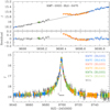 |
Fig. 1 Light curve of KMT-2022-BLG-0475. The lower panel shows the whole view, and the upper panel shows the enlarged view of the region around the anomaly. The arrow in the lower panel indicates the approximate time of the anomaly, tanom. The curve drawn over the data points is the model curve of the 1L1S solution. The KMTC data set is used for reference, to align the other data sets. |
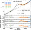 |
Fig. 2 Zoomed-in view around the anomaly in the lensing light curve of KMT-2022-BLG-0475. The lower three panels show the residuals from the finite-source close 2L1S model, the point-source close 2L1S model, and the 1L2S model. |
Model parameters for KMT-2022-BLG-0475.
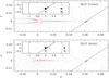 |
Fig. 3 Lens-system configurations of the close (upper panel) and wide (lower panel) 2L1S solutions of KMT-2022-BLG-0475. In each panel, the red cuspy figures are caustics and the line with an arrow represents the source trajectory. The whole view of the lens system is shown in the inset, in which the small filled dots indicate the positions of the lens components and the solid circle represents the Einstein ring. The gray curves surrounding the caustic represent equi-magnification contours. |
3.2 KMT-2022-BLG-1480
The lensing event KMT-2022-BLG-1480 occurred on a source lying at (RA, Dec)J2000 = (17:58:54.96, −29:28:23.99), which correspond to (l, b) = (1°.015, −2°.771). The event was first found by the KMTNet group on 2022 July 11 (HJD′ = 9771), when the source was brighter than the baseline magnitude, Ibase = 18.11, by ΔΙ ~ 0.65 mag. The source was in the KMTNet prime field BLG02, toward which observations were conducted with a 0.5 h cadence. This field overlaps with the BLG42 field in most region, but the source was in the offset region that was not covered by the BLG42 field. The event was also observed by the MOA and MAP survey groups, who observed event with a 0.2 hr cadence and a 0.5–1.0 day cadence, respectively.
In Fig. 4, we present the light curve of KMT-2022-BLG-1480. We found that a weak anomaly occurred about 3 days after the peak centered at tanom ~ 9793.2. The anomaly is characterized by a negative deviation in most part of the anomaly and a slight positive deviation in the beginning part centered at HJD′ ~ 9792.2. The anomaly, which lasted about 2.7 days, was covered by multiple data sets from KMTS, KMTA, and CFHT. The sky at the KMTC site was clouded out for two consecutive nights from July 30 to August 1 (9791 ≤ HJD′ ≤ 9793), and thus the anomaly was not covered by the KMTC data.
In Table 2, we present the best-fit lensing parameters of the 2L1S solution. We did not conduct 1L2S modeling because a negative deviation cannot be explained with a 1L2S interpretation. We found a pair of 2L1S solutions, in which one solution has binary parameters (s, q) ~ (0.83,4.9 × 10−4) and the other solution has parameters (s, q) ~ (1.03,4.7 × 10−4). Similar to the case of KMT-2022-BLG-0475L, the estimated mass ratio of order 10−4 is much smaller than the Jupiter/Sun mass ratio. As we discuss below, the similarity between the model curves of the two 2L1S solutions is caused by the inner-outer degeneracy, and thus we refer to the solutions as “inner” and “outer” solutions, respectively. From the comparison of the inner and outer solutions obtained under the assumption of a rectilinear relative lens-source motion, it was found that the outer model yields a substantially better fit than the fit of the inner model by Δχ2 = 63.9, indicating that the degeneracy was resolved. In Fig. 5, we present the model curves of the two solutions in the region around the anomaly. From the comparison of the models, it is found that the fit of the outer solution is better than the inner solution in the region around HJD′ ~ 9792, at which the anomaly exhibits slight positive deviations from the 1L1S model.
Figure 6 shows the lens-system configurations of the inner and outer 2L1S solutions. Although the fit is worse, we present the configuration of the inner solution in order to find the origin of the fit difference between the two solutions. The configuration shows that the outer solution results in a resonant caustic, in which the central and planetary caustics merge and form a single caustic, while the central and planetary caustics are detached in the case of the inner solution. According to the interpretations of both solutions, the source passed the back-end side of central caustic without caustic crossings. The configuration of the outer solution results in strong cusps lying on the back-end side, and this caustic feature explains the slight positive deviation appearing in the beginning part of the anomaly around HJD′ ~ 9792. 2. Similar to the case of KMT-2022-BLG-0475, finite-source effects were detected although the source did not cross the caustic. We plot the point-source model in Fig. 5 for the comparison with the finite-source model.
We find that the relation in Eq. (2) is also applicable to the two local solutions of KMT-2022-BLG-1480. With (sin, sout) ~ (0.82, 1.03), the fractional deviation of the value  from unity is
  . On the other hand, the fractional difference between
  and
and ![${s^\dag } = {{\left[ {{{\left( {u_{{\rm{anom}}}^2 + 4} \right)}^{{1 \mathord{\left/ {\vphantom {1 2}} \right. \kern-\nulldelimiterspace} 2}}} - {u_{{\rm{anom}}}}} \right]} \mathord{\left/ {\vphantom {{\left[ {{{\left( {u_{{\rm{anom}}}^2 + 4} \right)}^{{1 \mathord{\left/ {\vphantom {1 2}} \right. \kern-\nulldelimiterspace} 2}}} - {u_{{\rm{anom}}}}} \right]} {2 = 0.934\,{\rm{is}}\,{{{\rm{\Delta }}{s^\dag }} \mathord{\left/ {\vphantom {{{\rm{\Delta }}{s^\dag }} {{s^\dag } = 1.6\% }}} \right. \kern-\nulldelimiterspace} {{s^\dag } = 1.6\% }}}}} \right. \kern-\nulldelimiterspace} {2 = 0.934\,{\rm{is}}\,{{{\rm{\Delta }}{s^\dag }} \mathord{\left/ {\vphantom {{{\rm{\Delta }}{s^\dag }} {{s^\dag } = 1.6\% }}} \right. \kern-\nulldelimiterspace} {{s^\dag } = 1.6\% }}}} $](/articles/aa/full_html/2023/08/aa46667-23/aa46667-23-eq20.png) , which is 5 times smaller than that of the
, which is 5 times smaller than that of the  relation. This also indicates that the two local solutions result from the inner-outer degeneracy rather than the close–wide degeneracy. We also checked the Hwang et al. (2022) relation between the planet-to-host mass ratio and the lensing parameters for the “dip-type” anomalies,
 (5)
(5)
where Δtdip ~ 1.9 day is the duration of the dip in the anomaly. With the lensing parameters (tE, u0, s, α) = (26, 0.069, 1.03, 59°), we found that the mass ratio analytically estimated from Eq. (5) is q ~ 5.9 × 10⁻⁴, which is close to the value 4.6 × 10⁻⁴ found from the modeling.
We check whether the microlens-parallax vector πE = (πE,N, πE,E) can be measured by conducting extra modeling considering higher-order effects. We find that the inclusion of the higher-order effects improves the fit by Δχ2 = 6.9 with respect to the model obtained under the rectilinear lens-source motion (standard model). In Table 2, we list the lensing parameters of the pair of higher-order models with u0 > 0 and u0 < 0, which result from the mirror symmetry of the source trajectory with respect to the binary-lens axis (Skowron et al. 2011). The Δχ2 maps of the models on the (πE,E, πE,N) parameter plane obtained from the higher-order modeling are shown in Fig. 7. It is found that the maps of the solutions results in a similar pattern of a classical one-dimensional parallax ellipse, in which the east component πE,E is well constrained and the north component πE,N has a fairly big uncertainty. Gould et al. (1994) pointed out that the constraints of the one-dimensional parallax on the physical lens parameters are significant, and Han et al. (2016) indicated that the parallax constraint should be incorporated in the Bayesian analysis to estimate the physical lens parameters. We describe the detailed procedure of imposing the parallax constraint in the second paragraph of Sect. 5. While the parallax parameters (πE,N, πE,E) are constrained from the overall pattern of the light curve, the orbital parameters (ds/dt, dα/dt) are constrained from the anomaly induced by the lens companion. For KMT-2022-BLG-1480, the orbital parameters are poorly constrained because the duration of the planet-induced anomaly is very short.
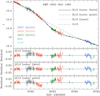 |
Fig. 5 Enlarged view around the anomaly in the lensing light curve of KMT-2022-BLG-1480. The lower three panels show the residuals form the inner 2L1S, the finite-source outer 2L1s, and point-source outer 2L1s models. |
Model parameters for KMT-2022-BLG-1480.
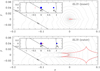 |
Fig. 6 Lens-system configurations for the inner and outer 2L1S solutions of KMT-2022-BLG-1480. Notations are same as those in Fig. 3. |
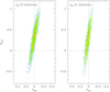 |
Fig. 7 Maps of Δχ2 on the (πΕ,E, πE,N) parameter plane for the higherorder u0 > 0 and u0 < 0 solutions of KMT-2022-BLG-1480. Points with ≤1σ are shown in red, ≤2σ in yellow, ≤3σ in green, ≤4σ in cyan, and ≤5σ in blue. |
Source properties, Einstein radii, and lens-source proper motions.
4 Source stars and angular Einstein radii
In this section, we constrain the source stars of the events to estimate the angular Einstein radii. Despite the non-caustic-crossing nature of the planetary signals, finite-source effects were detected for both events, and thus the normalized source radii were measured. With the measured value of ρ, we estimated the angular Einstein radius using the relation
 (6)
(6)
where the angular radius of the source was deduced from the reddening- and extinction-corrected (de-reddened) color and magnitude.
The left and right panels of Fig. 8 show the source locations in the instrumental color-magnitude diagrams (CMDs) of stars lying around the source stars of KMT-2022-BLG-0475 and KMT-2022-BLG-1480, respectively. For each event, the instrumental source color and magnitude, (V − I, I)S, were determined by estimating the flux values of the source fs and blend fb from the linear fit to the relation Fobs = A(t)fs + fb, where the lensing magnification is obtained from the model. We are able to constrain the blend for KMT-2022-BLG-1480 and mark its location on the CMD, but the blend flux of KMT-2022-BLG-0475 resulted in a slightly negative value, making it difficult to constrain the blend position. By applying the method of Yoo et al. (2004), we then estimated the de-reddened source color and magnitude, (V − I, I)0,S, using the centroid of the red giant clump (RGC), for which its de-reddened color and magnitude (V − I, I)0,RGC were known (Bensby et al. 2013; Nataf et al. 2013), as a reference, that is,
![${\left( {V - I,I} \right)_{0,{\rm{S}}}} = \left( {V - I,I} \right){ & _{{\rm{0,RGC}}}} + \left[ {{{\left( {V - I,I} \right)}_{\rm{S}}} - {{\left( {V - I,I} \right)}_{{\rm{RGC}}}}} \right].$](/articles/aa/full_html/2023/08/aa46667-23/aa46667-23-eq24.png) (7)
(7)
Here, (V − I, I)RGC denotes the instrumental color and magnitude of the RGC centroid, and thus the last term in the bracket represents the offset of the source from the RGC centroid in the CMD.
In Table 3, we summarize the values of (V − I, I)S, (V − I, I)RGC, (V − I, I)0,RGC, and (V − I, I)0,S for the individual events. From the estimated de-reddened colors and magnitudes, it was found that the source star of KMT-2022-BLG-0475 is an early K-type turnoff star, and that of KMT-2022-BLG-1480 is a late G-type subgiant. We estimated the angular source radius by first converting the measured V − I color into V − K color using the Bessell & Brett (1988) color-color relation, and then deducing θ* from the Kervella et al. (2004) relation between (V - K, V) and θ*. With the measured source radius, we then estimated the angular Einstein radius using the relation in Eq. (6) and the relative lens-source proper motion using the relation μ = θE/tE. The estimated θE and μ values of the individual events are listed in Table 3. We note that the uncertainties of the source colors and magnitudes presented in Table 3 are the values estimated from the model fitting, and those of θ* and θE are estimated by adding an additional 7% error to consider the uncertain de-reddened RGC color of Bensby et al. (2013) and the uncertain position of the RGC centroid (Gould 2014).
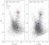 |
Fig. 8 Source locations of the lensing events KMT-2022-BLG-0475 (left panel) and KMT-2022-BLG-1480 (right panel) with respect to the positions of the centroids’ RGC in the instrumental CMDs of stars lying around the source stars of the individual events. For KMT-2022-BLG-1480, the position of the blend is also marked. |
5 Physical lens parameters
We determined the physical parameters of the planetary systems using the lensing observables of the individual events. For KMT-2022-BLG-0475, the measured observables are tE, and θΕ, which are respectively related to the mass and distance to the planetary system by
 (8)
(8)
where κ = 4G/(c2au) = 8.14 mas/M⊙. For KMT-2022-BLG-1480, we additionally measured the observable πΕ, with which the physical parameters can be uniquely determined by
 (9)
(9)
We estimated the physical parameters by conducting Bayesian analyses because the observable πΕ was not measured for KMT-2022-BLG-0475, and the uncertainty of the north component of the parallax vector, πΕ,Ν, was fairly big although the east component πΕ,Ε was relatively well constrained.
The Bayesian analysis was done by first generating artificial lensing events from a Monte Carlo simulation, in which a Galactic model was used to assign the locations of the lens and source and their relative proper motion, and a mass-function model was used to assign the lens mass. We adopted the Jung et al. (2021) Galactic model and the Jung et al. (2018) mass function. With the assigned values of (M, DL, DS,μ), we computed the lensing observables (tE,i, θΕ,i;,πΕ,i) of each simulated event using the relations in Eqs. (1) and (8). Under the assumption that the physical parameters are independently and identically distributed, we then constructed the Bayesian posteriors of M and DL by imposing a weight  . Here the
  value for each event was computed as
![$\chi _i^2 = {\left[ {{{{t_{{\rm{E,}}i}} - {t_{\rm{E}}}} \over {\sigma \left( {{t_{\rm{E}}}} \right)}}} \right]^2} + {\left[ {{{{\theta _{{\rm{E,}}i}} - {\theta _{\rm{E}}}} \over {\sigma \left( {{\theta _{\rm{E}}}} \right)}}} \right]^2} + \sum\limits_{j = 1}^2 {\sum\limits_{k = 1}^2 {{b_{\,j,k}}\left( {{\pi _{{\rm{E,}}j,i}} - {\pi _{{\rm{E,}}i}}} \right)\left( {{\pi _{{\rm{E,}}k,i}} - {\pi _{{\rm{E,}}i}}} \right),} } $](/articles/aa/full_html/2023/08/aa46667-23/aa46667-23-eq29.png) (10)
(10)
where (tE, θΕ, πΕ) represent the observed values of the lensing observables, [σ(tE), σ(θΕ)] denote the measurement uncertainties of tE and θΕ, respectively, denotes the inverse covariance matrix of πΕ, and (πE,1, πE,2)i = (πΕ,Ν, πΕ,Ε)i denote the north and east components of the microlens-parallax vector of each simulated event, respectively. We note that the last term in Eq. (10) was not included for KMT-2022-BLG-0475, for which the microlens-parallax was not measured.
In the case of the event KMT-2022-BLG-1480, for which the blending flux was measured, we additionally imposed the blending constraint that was given by the fact that the lens could not be brighter than the blend. In order to impose the blending constraint, we computed the lens magnitude as
 (11)
(11)
where MI,L represents the absolute I-band magnitude of a star corresponding to the lens mass, and AI,L represents the I-band extinction to the lens. For the computation of AI,L, we modeled the extinction to the lens as
![${A_{I{\rm{,L}}}} = {A_{I{\rm{,tot}}}}\,\left[ {1 - \exp \,\left( { - {{\left| z \right|} \over {{h_{z{\rm{,dust}}}}}}} \right)} \right],$](/articles/aa/full_html/2023/08/aa46667-23/aa46667-23-eq31.png) (12)
(12)
where AI,tot = 1.53 is the total I-band extinction toward the field, hz,dust = 100 pc is the vertical scale height of dust, z = DL sin b + z0, b is the Galactic latitude, and z0 = 15 pc is vertical position of the Sun above the Galactic plane (Siegert 2019). It turned out that the blending constraint had little effect on the posteriors because the other constraints, that is, those from (tE, θΕ, πΕ), already predicted that the planet host are remote faint stars whose flux contribution to the blended flux is negligible.
Figures 9 and 10 show the Bayesian posteriors of the lens mass and distances to the lens and source for KMT-2022-BLG-0475 and KMT-2022-BLG-1480, respectively. In Table 4, we summarize the estimated parameters of the host mass, Mh, planet mass, Mp, distance to the planetary system, projected separation between the planet and host, a⊥ = sθEDL, and the snow-line distances estimated as asnow ~ 2.7(M/M⊙) (Kennedy & Kenyon 2008). Here, we estimated the representative values and uncertainties of the individual physical parameters as the median values and the 16% and 84% range of the Bayesian posteriors, respectively.
We find that the two planetary systems KMT-2022-BLG-0475L and KMT-2022-BLG-1480L are similar to each other in various aspects. According to the estimated physical lens parameters, the masses of KMT-2022-BLG-0475Lb and KMT-2022-BLG-1480Lb are ~1.7 and ~1.8 times the mass of Uranus in our solar system. The planets are separated in projection from their hosts by ~2.0 au and ~1.2 au, respectively. The masses of planet hosts are ~0.43 M⊙ and ~0.18 M⊙, which correspond to the masses of early and mid-M dwarfs, respectively. Considering that the estimated separations are projected values and the snow-line distances of the planetary systems are asnow ~ 1.2 au for KMT-2022-BLG-0475Land ~0.5 au for KMT-2022-BLG-1480L, the planets of both systems are ice giants lying well beyond the snow lines of the systems. The planetary systems lie at distances of ~6.6 kpc and ~7.8 kpc from the Sun. The planetary systems are likely to be in the bulge, with a probability of 70% for KMT-2022-BLG-0475L and 83% for KMT-2022-BLG-1480L.
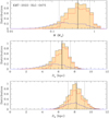 |
Fig. 9 Bayesian posteriors of the lens mass and distances to the lens and source for the lens system KMT-2022-BLG-0475L. In each panel, the solid vertical line represents the median value, and the two dotted vertical lines indicate the uncertainty range of the posterior distribution. The blue and red curves represent the contributions by the disk and bulge lens populations, respectively. |
Physical lens parameters.
6 Summary and conclusion
We analyzed the light curves of the microlensing events KMT-2022-BLG-0475 and KMT-2022-BLG-1480, for which weak short-term anomalies were found as part of a systematic investigation of the 2022 season data collected by high-cadence microlensing surveys. We tested various models that could produce the observed anomalies and found that they were generated by planetary companions to the lenses with a planet-to-host mass ratio q ~ 1.8 × 10⁻⁴ for KMT-2022-BLG-0475L and q ~ 4.3 × 10⁻⁴ for KMT-2022-BLG-1480L. From the physical parameters estimated from the Bayesian analyses using the observables of the events, we find that the planets KMT-2022-BLG-0475Lb and KMT-2022-BLG-1480Lb have masses ~1.7 and ~1.8 times the mass of Uranus, respectively, and they lie well beyond the snow lines of their hosts, which are early- and mid-M dwarfs, indicating that the planets are ice giants.
Surveys that use transit and radical velocity methods have difficulties detecting ice giants around M dwarf stars, not only because of the long orbital period of the planet but also because of the faintness of the host stars. The number of detected low-mass planets increases with the increasing observational cadence of microlensing surveys, as shown in the histogram of detected microlensing planets as a function of the planet-to-host mass ratio presented in Fig. 1 of Han et al. (2022c). High-cadence lensing surveys, which can complement transit and radical velocity surveys, will play an important role in the construction of a more complete planet sample and thus help us better understand the demographics of extrasolar planets.
The two events are also similar in that they have p measurements (and therefore also θE measurements) despite the fact that the source does not cross any caustics. Zhu et al. (2014) predicted that about half of KMT planets would not have caustic crossings, and Jung et al. (2023) confirmed this for a statistical sample of 58 planetary events detected during the 2018–2019 period. However, Gould (2022) shows that about one-third of non-caustic-crossing events nevertheless yield θE measurements.
Measurements of θE are important, not only because they improve the Bayesian estimates (see Sect. 5), but also because they allow accurate predictions of when high-resolution adaptive-optics (AO) imaging will be able to resolve the lens separately from the source, which will then yield mass measurements of both the host and the planet (Gould 2022). For KMT-2022-BLG-0475, with proper motion μ = 6.9 mas yr−1, the separation in 2030 (approximate first AO light on 30 m class telescopes) will be Δθ ~ 55 mas, which should be adequate to resolve the lens and source. Resolving the lens of this event would also be important for confirming the planetary interpretation of the event because it is difficult to completely rule out the 1L2S interpretation. By contrast, for KMT-2022-BLG-1480, with μ = 1.9 mas yr−1, the separation will be only Δθ ~ 15 mas, which almost certainly means that AO observations should be delayed for many additional years. In particular, if the Bayesian mass and distance estimates are approximately correct, then the expected contrast ratio between the source and lens is ΔΚ ~ 7 mag, which will likely require separations of at least four full widths at half maximum (i.e., 55 mas), even on the 39 m European Extremely Large Telescope. Hence, the contrast between the two planets presented in this paper underlines the importance of θE measurements.
Acknowledgements
Work by C.H. was supported by the grants of National Research Foundation of Korea (2019R1A2C2085965). This research has made use of the KMTNet system operated by the Korea Astronomy and Space Science Institute (KASI) at three host sites of CTIO in Chile, SAAO in South Africa, and SSO in Australia. Data transfer from the host site to KASI was supported by the Korea Research Environment Open NETwork (KREONET). This research was supported by the Korea Astronomy and Space Science Institute under the R&D program (Project No. 2023-1-832-03) supervised by the Ministry of Science and ICT. The MOA project is supported by JSPS KAKENHI Grant Number JSPS24253004, JSPS26247023, JSPS23340064, JSPS15H00781, JP16H06287, and JP17H02871. J.C.Y., I.G.S., and S.J.C. acknowledge support from NSF Grant No. AST-2108414. Y.S. acknowledges support from BSF Grant No. 2020740. This research uses data obtained through the Telescope Access Program (TAP), which has been funded by the TAP member institutes. W. Zang, H.Y., S.M., and W. Zhu acknowledge support by the National Science Foundation of China (Grant No. 12133005). W. Zang acknowledges the support from the Harvard-Smithsonian Center for Astrophysics through the CfA Fellowship. C.R. was supported by the Research fellowship of the Alexander von Humboldt Foundation.
References
- Albrow, M. D., Beaulieu, J.-P., Caldwell, J. A. R., et al. 2000, ApJ, 534, 894 [NASA ADS] [CrossRef] [Google Scholar]
- Bennett, D. P., & Rhie, S. H. 1996, ApJ, 472, 660 [NASA ADS] [CrossRef] [Google Scholar]
- Bensby, T., Yee, J. C., Feltzing, S. et al. 2013, A & A, 549, A147 [NASA ADS] [CrossRef] [EDP Sciences] [Google Scholar]
- Bessell, M. S., & Brett, J. M. 1988, PASP, 100, 1134 [Google Scholar]
- Bond, I. A., Abe, F., Dodd, R. J., et al. 2001, MNRAS, 327, 868 [Google Scholar]
- Gaudi, B. S., & Gould, A. 1997, ApJ, 486, 85 [Google Scholar]
- Gaudi, B. S., 1998, ApJ, 506, 533 [Google Scholar]
- Gould, A. 1992, ApJ, 392, 442 [Google Scholar]
- Gould, A. 2014, J. Korean Astron. Soc., 47, 153 [NASA ADS] [CrossRef] [Google Scholar]
- Gould, A. 2022, arXiv e-prints [arXiv:2209.12501] [Google Scholar]
- Gould, A., & Loeb, A. 1992, ApJ, 396, 104 [Google Scholar]
- Gould, A., Miralda-Escudé, J., & Bahcall, J. N. 1994, ApJ, 423, L105 [NASA ADS] [CrossRef] [Google Scholar]
- Gould, A., Han, C., Weicheng, Z., et al. 2022, A & A, 664, A13 [NASA ADS] [CrossRef] [EDP Sciences] [Google Scholar]
- Griest, K., & Safizadeh, N. 1998, ApJ, 500, 37 [Google Scholar]
- Han, C., Udalski, A., Gould, A., et al. 2016, ApJ, 828, 53 [NASA ADS] [CrossRef] [Google Scholar]
- Han, C., Gould, A., Albrow, M. D., et al. 2022a, A & A, 658, A62 [NASA ADS] [CrossRef] [EDP Sciences] [Google Scholar]
- Han, C., Bond, I. A., Yee, J., et al. 2022b, A & A, 658, A94 [NASA ADS] [CrossRef] [EDP Sciences] [Google Scholar]
- Han, C., Kim, D., Gould, A., et al. 2022c, A & A, 664, A33 [NASA ADS] [CrossRef] [EDP Sciences] [Google Scholar]
- Han, C., Kim, D., Yang, H., et al. 2022d, A & A, 664, A114 [NASA ADS] [CrossRef] [EDP Sciences] [Google Scholar]
- Han, C., Lee, C.-U., Gould, A., et al. 2022e, A & A, 666, A132 [NASA ADS] [CrossRef] [EDP Sciences] [Google Scholar]
- Han, C., Gould, A., Jung, Y. K., et al. 2023a, A & A, 674, A89 [NASA ADS] [CrossRef] [EDP Sciences] [Google Scholar]
- Han, C., Udalski, A., Jung, Y. K., et al. 2023b, A & A, 670, A172 [NASA ADS] [CrossRef] [EDP Sciences] [Google Scholar]
- Hwang, K.-H., Zang, W., Gould, A., et al. 2022, AJ, 163, 43 [NASA ADS] [CrossRef] [Google Scholar]
- Jung, Y. K., Udalski, A., Gould, A., et al. 2018, AJ, 155, 219 [Google Scholar]
- Jung, Y. K., Han, C., Udalski, A., et al. 2021, AJ, 161, 293 [NASA ADS] [CrossRef] [Google Scholar]
- Jung, Y. K., Zang, W., Han, C., et al. 2022, AJ, 164, 262 [NASA ADS] [CrossRef] [Google Scholar]
- Jung, Y. K., Zang, W., Wang, H., et al. 2023, AJ, 165, 226 [NASA ADS] [CrossRef] [Google Scholar]
- Kennedy, G. M., & Kenyon, S. J. 2008, ApJ, 673, 502 [Google Scholar]
- Kervella, P., Thévenin, F., Di Folco, E., & Ségransan, D. 2004, A & A, 426, 29 [Google Scholar]
- Kim, S.-L., Lee, C.-U., Park, B.-G., et al. 2016, JKAS, 49, 37 [Google Scholar]
- Kruszyńska, K., Wyrzykowski, Ł., Rybicki, K. A., et al. 2022, A & A, 662, A59 [CrossRef] [EDP Sciences] [Google Scholar]
- Luberto, J., Martin, E. C., McGill, P., Leauthaud, A., Skemer, A. J., & Lu, J. R. 2022, AJ, 164, 253 [NASA ADS] [CrossRef] [Google Scholar]
- Medford, M. S., Abrams, N. S., Lu, J. R., Nugent, P., & Lam, C. Y. 2023, ApJ, 947, 24 [Google Scholar]
- Mao, S., & Paczyński, B. 1991, ApJ, 374, 37 [Google Scholar]
- Nataf, D. M., Gould, A., Fouqué, P. et al. 2013, ApJ, 769, 88 [Google Scholar]
- Rodriguez, A. C., Mróz, P., Kulkarni, S. R., et al. 2022, ApJ, 927, 150 [Google Scholar]
- Sahu, K. C., Anderson, J., Casertano, S., et al. 2022, ApJ, 933, 83 [Google Scholar]
- Shin, I.-G., Yee, J., Zang, W., et al. 2023, AAS, submitted [arXiv:2303.16881] [Google Scholar]
- Siegert, T. 2019, A & A, 632, A1 [Google Scholar]
- Skowron, J., Udalski, A., Gould, A., et al. 2011, ApJ, 738, 87 [Google Scholar]
- Tonry, J. L., Denneau, L., Heinze, A. N., et al. 2018, PASP, 130, 064505 [Google Scholar]
- Udalski, A., Kubiak, M., Szymański, M., et al. 1994, Acta Astron., 44, 317 [Google Scholar]
- Wang, H., Zang, W., Zhu, W., et al. 2022, MNRAS, 510, 1778 [Google Scholar]
- Yee, J. C., Shvartzvald, Y., Gal-Yam, A., et al. 2012, ApJ, 755, 102 [Google Scholar]
- Yoo, J., DePoy, D.L., Gal-Yam, A. et al. 2004, ApJ, 603, 139 [NASA ADS] [CrossRef] [Google Scholar]
- Zang, W., Han, C., Kondo, I., et al. 2021a, RA & A, 21, 239 [Google Scholar]
- Zang, W., Hwang, K.-H., Udalski, A., et al. 2021b, AJ, 162, 163 [NASA ADS] [CrossRef] [Google Scholar]
- Zang, W., Yang, H., Han, C., et al. 2022, MNRAS, 515, 928 [NASA ADS] [CrossRef] [Google Scholar]
- Zang, W., Jung, Y.K., Yang, H., et al. 2023, AJ, 165, 103 [CrossRef] [Google Scholar]
- Zhu, W., Penny, M., Mao, S., Gould, A., & Gendron, R. 2014, ApJ, 788, 73 [Google Scholar]
The Optical Gravitational Microlensing Experiment (OGLE: Udalski et al. 1994) is another major microlensing survey, although the two events analyzed in this work were not detected by the survey because the OGLE telescope was not operational in the first half of the 2022 season. Besides these surveys dedicated to the microlensing program, lensing events are detected from other surveys such as the Zwicky Transient Facility (ZTF) survey (Rodriguez et al. 2022; Medford et al. 2023) and the Asteroid Terrestrial-impact Last Alert System (ATLAS) survey (Tonry et al. 2018), or observed using space-based instrument such as the Gaia survey (Kruszyńska et al. 2022; Luberto et al. 2022) and Hubble Space Telescope (Sahu et al. 2022).
All Tables
All Figures
|
Fig. 1 Light curve of KMT-2022-BLG-0475. The lower panel shows the whole view, and the upper panel shows the enlarged view of the region around the anomaly. The arrow in the lower panel indicates the approximate time of the anomaly, tanom. The curve drawn over the data points is the model curve of the 1L1S solution. The KMTC data set is used for reference, to align the other data sets. |
| In the text | |
|
Fig. 2 Zoomed-in view around the anomaly in the lensing light curve of KMT-2022-BLG-0475. The lower three panels show the residuals from the finite-source close 2L1S model, the point-source close 2L1S model, and the 1L2S model. |
| In the text | |
|
Fig. 3 Lens-system configurations of the close (upper panel) and wide (lower panel) 2L1S solutions of KMT-2022-BLG-0475. In each panel, the red cuspy figures are caustics and the line with an arrow represents the source trajectory. The whole view of the lens system is shown in the inset, in which the small filled dots indicate the positions of the lens components and the solid circle represents the Einstein ring. The gray curves surrounding the caustic represent equi-magnification contours. |
| In the text | |
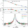 |
Fig. 4 Light curve of the lensing event KMT-2022-BLG-1480. Notations are same as those in Fig. 1. |
| In the text | |
|
Fig. 5 Enlarged view around the anomaly in the lensing light curve of KMT-2022-BLG-1480. The lower three panels show the residuals form the inner 2L1S, the finite-source outer 2L1s, and point-source outer 2L1s models. |
| In the text | |
|
Fig. 6 Lens-system configurations for the inner and outer 2L1S solutions of KMT-2022-BLG-1480. Notations are same as those in Fig. 3. |
| In the text | |
|
Fig. 7 Maps of Δχ2 on the (πΕ,E, πE,N) parameter plane for the higherorder u0 > 0 and u0 < 0 solutions of KMT-2022-BLG-1480. Points with ≤1σ are shown in red, ≤2σ in yellow, ≤3σ in green, ≤4σ in cyan, and ≤5σ in blue. |
| In the text | |
|
Fig. 8 Source locations of the lensing events KMT-2022-BLG-0475 (left panel) and KMT-2022-BLG-1480 (right panel) with respect to the positions of the centroids’ RGC in the instrumental CMDs of stars lying around the source stars of the individual events. For KMT-2022-BLG-1480, the position of the blend is also marked. |
| In the text | |
|
Fig. 9 Bayesian posteriors of the lens mass and distances to the lens and source for the lens system KMT-2022-BLG-0475L. In each panel, the solid vertical line represents the median value, and the two dotted vertical lines indicate the uncertainty range of the posterior distribution. The blue and red curves represent the contributions by the disk and bulge lens populations, respectively. |
| In the text | |
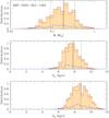 |
Fig. 10 Bayesian posteriors of KMT-2022-BLG-1480. Notations are same as those in Fig. 9. |
| In the text | |
Current usage metrics show cumulative count of Article Views (full-text article views including HTML views, PDF and ePub downloads, according to the available data) and Abstracts Views on Vision4Press platform.
Data correspond to usage on the plateform after 2015. The current usage metrics is available 48-96 hours after online publication and is updated daily on week days.
Initial download of the metrics may take a while.