| Issue |
A&A
Volume 673, May 2023
|
|
|---|---|---|
| Article Number | A163 | |
| Number of page(s) | 18 | |
| Section | The Sun and the Heliosphere | |
| DOI | https://doi.org/10.1051/0004-6361/202245701 | |
| Published online | 24 May 2023 | |
Photospheric signatures of retraction and reconnection in realistic magnetohydrodynamic simulations
1
Leibniz-Institut für Sonnenphysik (KIS), Schöneckstr. 6, 79104 Freiburg, Germany
2
Racah Institute of Physics, The Hebrew University of Jerusalem, Jerusalem, 91904
Israel
e-mail: This email address is being protected from spambots. You need JavaScript enabled to view it.
Received:
16
December
2022
Accepted:
9
March
2023
Abstract
Context. Magnetic flux emergence and cancelling in the quiet Sun is a frequently observed phenomenon. The two possible physical flux-removal mechanisms involved in this cancelling process are retraction and reconnection.
Aims. We seek to find distinct observational signatures characterising retraction and reconnection.
Methods. We carried out three-dimensional non-grey radiative magnetohydrodynamic (MHD) simulations of convection near the solar surface and the solar photosphere using the STAGGER code, and employing different initial conditions: (1) mixed-polarity simulations with alternating horizontal stripes of opposite vertical magnetic field and separated by a zero field stripe, and (2) flux emergence simulations with continuous injection of magnetic flux from the lower boundary. These initial conditions are meant to represent two different situations in the solar photosphere, namely magnetic flux cancelling in the absence or presence of magnetic flux emergence, respectively.
Results. We analyse the observational signatures of magnetic flux-removal processes for flux emergence as well as for mixed-polarity MHD simulations. In the flux emergence simulation, we are able to identify ubiquitous reconnection events anywhere from the solar surface to the upper photosphere. For a few of those reconnection events, we can identify supersonic upflow velocities in the upper photosphere as well as strong temperature enhancements. We also see strong electric currents very close to the locations where reconnection takes place, as well as supersonic horizontal velocities leading to sideways plasma compression. In the mixed-polarity simulations, we only detect observational signatures of magnetic field retraction related to large downflow velocities that appear in between regions where opposing horizontal velocities converge. These horizontal velocities are often supersonic, leading to heating due to shock dissipation. We do not see clear signatures of magnetic reconnection in these mixed-polarity simulations.
Conclusions. We suggest that, in the emerging flux regions of the quiet Sun, the main flux-removal process is reconnection, while in regions without flux emergence, retraction is the dominant flux-removal process.
Key words: magnetic reconnection / Sun: photosphere / Sun: magnetic fields
© The Authors 2023
 Open Access article, published by EDP Sciences, under the terms of the Creative Commons Attribution License (https://creativecommons.org/licenses/by/4.0), which permits unrestricted use, distribution, and reproduction in any medium, provided the original work is properly cited.
This article is published in open access under the Subscribe to Open model. This email address is being protected from spambots. You need JavaScript enabled to view it. to support open access publication.
1. Introduction
The magnetic flux that emerges in new active regions throughout a sunspot cycle has largely disappeared from the solar surface at the cycle minimum, with the remaining magnetic flux having travelled towards the poles (see Fig. 17 in Hathaway 2015). Howard & Labonte (1981) observed flux-emerging regions of this kind and concluded that newly erupted flux disappears from view in about 10 days. In the standard picture developed by Zwaan (1987, Fig. 2), the magnetic flux removal from the solar surface happens due to either magnetic reconnection –above or below the photosphere– or retraction. In this simple schematic describing reconnection, two initially vertical magnetic field lines of opposite polarity get close enough to each other to reconfigure their magnetic field, forming Ω-loops pulling down below the photosphere and U-loops propagating upwards in the higher atmosphere after reconnection. Following this scenario, strong plasma flows are expected. Furthermore, a measurable amount of temperature increase was detected by Cameron et al. (2011) in realistic 3D magnetohydrodynamic (MHD) near-surface simulations for reconnection. However, the observational signatures depend on the magnetic field geometry and will appear different for magnetic field configurations deviating from the aforementioned example.
The other mechanism for magnetic flux removal in the description provided by Zwaan is retraction. This describes the process where initially connected magnetic field lines can be pulled down below the surface, either through advection by plasma flows, or through the help of the radially inward-pointing magnetic curvature force, which can pull an Ω-loop down if the footpoints of those opposite-polarity magnetic fields are close enough to each other so that the curvature radius becomes small and the downwards pulling force strong. For magnetic flux that has already been at the solar surface for a long time, this mechanism is supposed to be at play, because the flux has had time to reconnect to the preexisting field, and is set up in a potential configuration. The observational signatures expected in the case of retraction are strong vertical downflows and horizontal inflows, but no strong upflows. Furthermore, a temperature increase can be expected from the compression of the material attached to the magnetic field lines that are pulled downwards, as has been shown in 3D MHD near-surface simulations by Thaler & Spruit (2017).
However, in reality, the situation is more complicated than described in the simplistic picture above. As high-resolution images of the quiet Sun reveal, even in the quiet Sun, magnetic flux emergence and flux cancelling are ubiquitous (Borrero et al. 2010; Solanki et al. 2010). This means that the magnetic field geometry and time evolution at the flux-removal sites might be complex and often unresolved in observations because of the lack of spacial or temporal resolution as well as the lack of multi-height observations. The lower solar atmosphere (i.e. photosphere) is usually described by ideal MHD, where reconnection does not occur. However, in localised regions, non-ideal effects can play a role, and the current density can be sufficiently high for reconnection to occur when opposite-polarity fields are close to each other and form current sheets (Pontin & Priest 2022). Whether magnetic reconnection can be detected or not will depend on the amount of energy released per unit mass. Priest et al. (2018) suggested that photospheric flux cancelling due to reconnection, which is sometimes referred to as nanoflares, might be driving magnetic reconnection at the base of the chromosphere and therefore be responsible for chromospheric heating (further elaborated in Priest & Syntelis 2021).
As described above, in observations, the two flux-removal processes, retraction and reconnection, can often not be disentangled from each other. However, it would be very useful to investigate whether or not their signatures can be distinguished from one another if data availability is not an issue, as in realistic MHD simulations. To this end, here we compare the observational signatures of reconnection and retraction events in the quiet Sun in order to characterise their unique features. It is hoped that these characterisations will help observers to identify such events in the future. This paper is organised as follows. In Sect. 2 we describe the numerical code and boundary conditions employed to simulate the two aforementioned flux-removal processes. In Sect. 3 we statistically analyse the physical parameters (magnetic field, velocity, temperature, and so forth) of the performed simulations. Section 4 presents a detailed study of individual cases of retraction and reconnection. Finally, we summarise our findings in Sect. 5.
2. Calculations
2.1. Numerical methods
The numerical simulations were realised with the 3D MHD code STAGGER (Galsgaard & Nordlund 1996). This code solves the time-dependent MHD equations by a sixth-order finite difference scheme using fifth-order interpolations for the spatial derivatives, while the time evolution is calculated using a third-order Runge-Kutta scheme. For every time step, the radiative-transfer equation is solved at every grid point assuming local thermal equilibrium. This is done using a Feautrier-like scheme along the rays with two μ angles plus the vertical and four ϕ angles horizontally, which adds up to nine angles in total. To incorporate the wavelength dependence of the absorption coefficient, the Planck function is sorted into four opacity bins. The equation-of-state table is calculated using a standard program for ionisation equilibria and absorption coefficients (Gustafsson 1973) and using opacity distribution functions identical to those used by Gustafsson et al. (1975), which are described in more detail in Nordlund (1982), Nordlund & Stein (1990), Stein & Nordlund (1998). For a more detailed description of the STAGGER code, see Beeck et al. (2012).
In this work, simulation runs were performed with periodic horizontal boundaries. At the top and bottom we have open transmitting boundaries. Convection is mostly driven by radiative cooling at the solar surface leading to an average convectively unstable temperature stratification according to the Schwarzschild criterion, as described in great detail in Nordlund et al. (2009). The main role of the lower boundary of the convection zone (in our case the lower boundary of the box), is to provide heat, which we note is not the main driver of convection on local scales (details in the same review.) Therefore, the effective surface temperature resulting from the model is controlled by setting the density and temperature of the inflowing gas through the lower boundary to a constant value, which determines the gases entropy value at this location. In addition, the magnetic field at the lower boundary is set to a constant value (in any field direction) for the inflowing material, while at the top boundary a potential field extrapolation is applied.
In all simulation runs, the size of the domain is 12 × 12 × 3.3 Mm3 in the (x, y, z) directions, respectively. The direction of the solar gravity acceleration is the z-axis. z = 0 is defined as the average location where the Rosseland-opacity τR = 1 is located. Below this point (i.e. towards the convection zone), we define z > 0, whereas above it (i.e. towards the photosphere), z < 0. With this definition vz < 0 and vz > 0 indicate upflows and downflows, respectively. The grid sizes are: Δx = Δy = 25 km. Here, Δz varies from approximately 33 km in the convection zone to 7 km around the τR = 1 layer. The total number of grid points in the simulation domain is 480 × 480 × 220. The physical properties of a typical hydrodynamical snapshot are depicted in Figs. A.1 and A.2.
2.2. Setup
2.2.1. Mixed-polarity field simulations: retraction setup
The setup designed to test the physical process of magnetic field retraction is the following: on top of a hydrodynamically relaxed snapshot, we impose four 3 Mm-wide stripes along the x-direction with Bz > 0, Bz = 0, Bz < 0, and Bz = 0. Initially, the stripes fill the entire domain along the y- and z-directions.
Our mixed-polarity magnetic field setup was inspired by Cameron et al. (2011). A similar setup was later applied in Thaler & Spruit (2017). The former authors interpreted the flux cancellation at the boundaries between the opposite-polarity fields as being dominantly caused by reconnection processes. Using a similar setup, Thaler & Spruit (2017) interpreted the strong flux-cancelling signatures at the border of the two polarities during the first few minutes of simulation run time as a signature of magnetic-field retraction. In the current paper, the choice to have an additional field free stripe in between the regions of opposite-polarity vertical magnetic fields was made to avoid any initial flux-cancelling behaviour at the border between the two polarities, which is difficult to interpret.
The mixed-polarity simulation was run twice, once for an initial vertical field of ‖Bz,init‖ = 1000 G and a second time with an initial vertical magnetic field of ‖Bz,init‖ = 200 G. The former run evolved for 100 min, whereas the latter evolved for 118 min. The temporal resolution of our output data was 10 s for all runs. This high output cadence represents an attempt to detect the observational signatures of reconnection, which are very transient if they happen close to the upper boundary. This is to be compared with the 30 s output cadence in Cameron et al. (2011).
2.2.2. Single-polarity field simulations: Comparison setup
To make sure that any characteristic features –such as enhanced vertical or horizontal flows– are due to magnetic flux cancelling and not simply the presence of magnetic fields even in the absence of flux removal, we carried out a comparison setup. The comparison setup appears identical to the mixed-polarity simulation run (Sect. 2.2.1), with the important difference that we are not superimposing vertical magnetic fields of alternating polarity on a hydrodynamical snapshot, but magnetic fields of only one polarity (Bz,init > 0 always). Otherwise the setup is identical to the mixed-polarity setup in terms of the stripe configuration, initial field strengths (1000 G and 200 G), and the time length of the simulations. However, the presence of only one magnetic-field polarity ensures that no magnetic flux-removal processes can take place.
2.2.3. Flux emergence simulations: Reconnection setup
The setup used to test the physical process of reconnection is such that, at the deepest 160 km in the vertical direction of the simulation box, a horizontal magnetic field with a strength of Bh = 1 kG (Bx = 500, By = 866 G) was superimposed to the hydrodynamically relaxed snapshot. In addition, we set the horizontal magnetic field strength of the inflowing material at the lower boundary to 1 kG with the same Bx and By values. This simulation was run for 165 min with a temporal resolution of 10 s.
3. Results
3.1. Temporal evolution of magnetic flux/energy
In Fig. 1 we see the time evolution of the magnetic energy in the mixed-polarity simulations divided by the magnetic energy of the same run at t = 0 s. Within the first 40 min, the magnetic energy is amplified because of convective motions in the ‖Bz,init‖ = 200 G setup (blue). However, in the ‖Bz,init = 1000‖ G setup (green), convective motions are suppressed because the initial magnetic field strength is above the equipartition value, and consequently the magnetic energy grows only during the first 500 s.
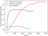 |
Fig. 1. Natural logarithm of magnetic energy integrated over the whole simulation box and normalised to the initial magnetic energy value for each simulation. The mixed-polarity simulation with ‖Bz,init‖ = 200 G is shown in blue, whereas green shows ‖Bz,init‖ = 1000 G. The flux emergence simulation is depicted in red. |
Figure 1 also shows that the timescale of the magnetic-flux-removal process strongly depends on the initial magnetic-field strength. This can be explained by the fact that the main flux-removal process in the mixed-polarity setup is retraction assisted by radially inward-pointing magnetic-tension forces, which increase with the square of the magnetic-field strength. As the mixed-polarity simulation setup had the 3 Mm-wide stripes with Bz = 0 in between the two polarities, the initially vertical magnetic field of 200 G and 1000 G, respectively, first forms magnetic bright points that then slowly approach each other due to advection by granular motions, thereby starting the retraction process.
3.2. Observational signatures of retraction and reconnection at τR = 1 and τR = 2 × 10⁻³
Figures 2 and 3 show the time evolution of the ‖Bz,init‖ = 1000 G mixed-polarity run (Sect. 2.2.1) at τR = 1 and τR = 2 × 10⁻³ layers, respectively. From the top panel of Fig. 2, we see that at t = 10 min the vertical magnetic field of the two polarities still mostly resembles the initial stripe-like structure. The difference is that at many locations, it has gathered in kilogauss magnetic structures instead of a homogeneous vertical field.
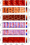 |
Fig. 2. Temporal evolution of the physical parameters at τR = 1 in the ‖Bz,init‖ = 1000 G mixed-polarity setup (Sect. 2.2.1). From top to bottom: Bz, |

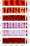 |
Fig. 3. Same as Fig. 2 but at τR = 2 × 10⁻³ (i.e. higher up in the photosphere and closer to the upper boundary). |
In the second panel from the top, we can clearly identify enhanced horizontal fields, Bh, between the opposite Bz (first panel) polarities for the first 20 min of the simulation run. This is expected, as the potential field boundary condition ensures that field lines of opposite Bz are connected horizontally above the photosphere from the beginning of the simulation run. In these regions of enhanced horizontal fields, strong vertical downflows (vz > 0) develop. This is demonstrated in the panels on the fifth row of Figs. 2 and 3. These downflows are surrounded by strong converging inflows along the x-direction, vx (fourth row). The regions of strong downflows correspond to a temperature enhancement at τR = 2 × 10⁻³ (sixth row in Fig. 3). The third panel, which shows the time evolution of the absolute value of the total magnetic field, clearly indicates flux removal, which is most clearly visible at t = 60 min at the x = 4 Mm stripe where the strong downflows and inflows have occurred at t = 10 min.
These results are in agreement with the retraction picture of flux cancelling, where field lines are already initially connected with each other and they are removed from the surface without any signatures of reconnection. A similar behaviour can be found for the mixed-polarity simulation run with weaker field, ‖Bz,init‖ = 200 G, but on longer timescales (see Figs. B.1 and B.2).
Figures 4 and 5 show similar plots to Figs. 2 and 3 but illustrate the time evolution of the flux-emergence simulation (Sect. 2.2.3). The magnetic field evolution in both figures (panels 1–3) shows that it takes time for the magnetic field to reach the surface, which means that at 20 min there is no magnetic flux at the surface yet, while at 70 min it has gathered in the intergranular lanes, and after 120 min enough flux has accumulated to form magnetic bright points.
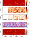 |
Fig. 4. Temporal evolution of the physical parameters at τR = 1 in the flux-emergence setup (Sect. 2.2.3). From top to bottom: Bz, |

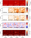 |
Fig. 5. Same as Fig. 4 but at τR = 2 × 10⁻³ (i.e. higher up in the photosphere and closer to the upper boundary). |
At τR = 1 (Fig. 4), the pattern of vertical velocity (fourth row) and temperature (fifth row) closely resembles that of regular granulation: hot upflows and cool downflows with superimposed bright points at those locations where the magnetic field concentrates. At τR = 2 × 10⁻³ (Fig. 5), the pattern is that of reversed granulation: cool upflows and hot downflows. The small square box in the third column in these two plots shows the location of a reconnection event first noticed as a spatially large upflow with vz ≈ −12 km s−1 in the upper photosphere lying on top of what appears as a granule at τR = 1. This particular event is studied in detail in Sect. 4.2. Figure 6 depicts the time evolution of the absolute value of the magnetic field within the aforementioned box, and shows that although overall the magnetic field grows over time in the flux emergence simulation, locally it can still decrease as in this example.
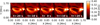 |
Fig. 6. Temporal evolution of the absolute value of the magnetic field |Btot| for the flux-cancelling event described in Sect. 2.2.3 in the flux-emergence setup at τR = 2 × 10⁻³. |
3.3. Statistical properties of reconnection and retraction simulations
In Figs. 7 and 8, we show a comparison of the statistical properties of the single-polarity simulation runs (Sect. 2.2.2), the mixed-polarity setups (Sect. 2.2.1) with different initial field strengths (‖Bz,init‖ = 200,1000 G), and the flux-emergence simulation (Sect. 2.2.3). We compute the histograms for the mixed-polarity and single-polarity simulations by taking 10 s cadence snapshots, starting 10 min after the beginning of the simulation until the end of it. The flux emergence histograms are produced in the same way, but this time the starting point is 100 min after the beginning of the simulation, as it takes time for the magnetic flux to rise and accumulate at the surface (see uppermost panels of Figs. 4 and 5).
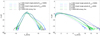 |
Fig. 7. Probability distributions of the vertical velocity vz (left panel) and the horizontal velocity |
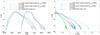 |
Fig. 8. Probability distributions of the temperature (left panel) and the horizontal magnetic field Bh (right panel). Results for the mixed-polarity and single-polarity runs (Sect. 2.2.3) with ‖Bz,init‖ = 1000 G are shown in solid cyan and dashed cyan for τR = 1 and solid blue and dashed blue for τR = 2 × 10⁻³, respectively, whereas results for the run with ‖Bz,init‖ = 200 G are indicated in solid emerald green and dashed emerald green for τR = 1 and solid green and dashed green for τR = 2 × 10⁻³, respectively. The flux-emergence simulation results are shown in black for τR = 1 (solid) and τR = 2 × 10⁻³ (dashed). |
In this section, we would like to answer two main questions. The first is whether the physical signatures of the retraction process can be distinguished from those in the reconnection process given data availability at high spatial resolution and high temporal cadence. The second question we want to address is whether or not the physical signatures of retraction in the mixed-polarity simulations can be uniquely identified and whether or not they are absent in the comparison simulations (single-polarity simulations) where no flux-removal process takes place. The retraction signatures we expect to see are uniquely strong downflows and horizontal inflows as well as a temperature enhancement similar to the one found by Thaler & Spruit (2017).
The reconnection signatures we expect to see in our simulation runs are different from the picture described by Zwaan (1987) and summarised in Sect. 1: we do not necessarily encounter the simplistic picture of two vertical magnetic field lines of opposite polarity that meet and reconnect. In the flux-emergence simulations, we do have a horizontal flux sheet injected from the lower boundary, which is then advected by the granular motions towards the surface and gathers in the intergranular lanes. Because of the advection process, the magnetic fields get amplified, tweaked, and twisted in the intergranules, whereby opposite polarities often come into close proximity. At the boundaries of the different magnetic field polarities, we expect current sheets to form, which ultimately lead to reconnection if the current density is high enough. The magnetic energy released due to reconnection leads to heating of the surrounding plasma, therefore we do expect a temperature increase to happen where reconnection takes place. However, the details depend not only on the current density but also on the density of the surrounding plasma. During reconnection events, diverging, possibly supersonic velocities can be detected, with their specific direction depending on the geometry of the magnetic field configuration.
Figure 7 reveals that the vertical velocity distribution of the flux-emergence simulation at τR = 2 × 10⁻³ (dashed black) has uniquely high upflow (vz < 0) velocities, reaching supersonic values of 8 − 12 km s−1. At τR = 1, supersonic upflow velocities of 8 − 10 km s−1 can be detected for the flux-emergence simulations (solid black lines on the left panel of Fig. 7). For the mixed-polarity simulations, the highest upflow velocities detected are 10 km s−1, and are reached at τR = 1 for both simulation setups (solid cyan: ‖Bz,init‖ = 1000 G; solid emerald green: ‖Bz,init‖ = 200 G); these values are almost identical to the single-polarity runs at the same optical depth (as shown in dashed cyan and dashed emerald green respectively). At τR = 2 × 10⁻³, the 10 km s−1 velocities are only reached in the mixed-polarity run with ‖Bz,init‖ = 200 G (solid green).
In both setups (i.e. mixed-polarity run with ‖Bz,init‖ = 1000 G, ‖Bz,init‖ = 200 G and the flux-emergence run), supersonic downflow (vz > 0) velocities appear. We find that the mixed-polarity simulations with ‖Bz,init‖ = 1000 G (solid cyan for τR = 1 and solid blue for τR = 2 × 10⁻³) show much higher peak values for the downflow velocity (up to 17 km s−1 at all τR-levels) compared to the single-polarity run (up to 11 km s−1; dashed cyan and dashed blue). The mixed-polarity simulations with an initial field strength of 200 G (left panel Fig. 7) exhibit enhanced downflow velocities (up to 14 km s−1) compared to the corresponding single-polarity run (up to 12 km s−1) only at τR = 2 × 10⁻³ (solid green vs. dashed green), while at τR = 1, the two runs look very similar (solid emerald green vs. dashed emerald green). We interpret the enhanced downflow velocities in the mixed-polarity simulations over the corresponding single-polarity simulation as retraction signatures. This addresses the second question that was originally posed.
The right panel of Fig. 7 reveals the presence of supersonic horizontal velocities in all setups, even though the single-polarity runs have smaller values than the mixed-polarity and flux emergence simulations. The solid blue line indicates that, for ‖Bz,init‖ = 1000 G, the peak horizontal velocities reach up to 15 km s−1 at τ = 2 × 10⁻³ compared to 11 km s−1 at the same optical depth in the single-polarity run (dashed blue line). The peak horizontal velocities go hand in hand with the peak horizontal field strength values, as depicted in the right panel of Fig. 8. Here, we see horizontal field strengths of about 50% higher in the mixed-polarity run with ‖Bz,init‖ = 1000 G (solid cyan) compared to the single-polarity run (dashed cyan) at τr = 1, while at τr = 2 × 10⁻³ (solid blue vs. dashed blue) they only differ by around 30%. Meanwhile, for ‖Bz,init‖ = 200 G, the single-polarity and mixed-polarity runs are almost identical in the horizontal velocities and are very similar in the horizontal fields (solid and dashed emerald green lines (τR = 1) and solid and dashed green lines (τR = 2 × 10⁻³) in the right panel of Fig. 8).
In the left panel of Fig. 8, the temperature distribution for the different setups is shown. We note that the temperature enhancement of the mixed-polarity setups (solid cyan, blue, emerald green and green) over the single-polarity setups (dashed cyan, blue, emerald green and green) is largest at τR = 2 × 10⁻³ for ‖Bz,init‖ = 1000 G (solid blue line vs. dashed blue line), with the former featuring maximum temperatures of about 8000 K, while the maximum temperatures at τR = 2 × 10⁻³ in the single-polarity run (Sect. 2.2.2) are up to 7000 K. The temperature distributions for the mixed-polarity run with ‖Bz,init‖ = 200 G (right panel in Fig. 8, solid emerald green) do not exhibit any significant difference with respect to their single-polarity counterpart (dashed emerald green).
These temperature enhancements are a consequence of the retraction process, and can be attributed to the dissipated energy due to the converging flows, as further described in Sect. 4.1 (see also Fig. 10). Furthermore, the cooler temperatures of the Bz,init = 1000 G single-polarity simulation (dashed cyan for τR = 1 and dashed blue for τR = 2 × 10⁻³) in the left panel of Fig. 8 compared to the Bz,init = 200 G single-polarity simulation (dashed emerald green for τR = 1 and dashed green for τR = 2 × 10⁻³) are a consequence of the enhanced suppression of convection with stronger vertical magnetic field, which leads to less heat transport to the surface layers. The fact that the flux emergence simulation at τR = 1 possesses higher temperatures (> 8000 K) than the mixed or single-polarity runs could be attributed to either the absence of strong large-scale vertical magnetic fields or to ohmic and compressional heating in reconnection events occurring in the deep photosphere. An example of such an event in the upper photosphere is discussed in Sect. 4.2.
In summary, we find uniquely high downflow velocities and temperature enhancements in the mixed-polarity setups (Sect. 2.2.1), which are absent in the control setup (Sect. 2.2.2) and can be attributed to the retraction process. Furthermore, we find distinct, highly supersonic vertical upflow velocities in the flux-emergence simulations (Sect. 2.2.3), which we attribute to magnetic reconnection processes in the upper photosphere.
4. Event analysis
In Sect. 3.2, we focus on the statistical analysis and description of the simulation results in the mixed-polarity field (Sect. 2.2.1), single-polarity field (Sect. 2.2.2), and the flux emergence setup (Sect. 2.2.3). In this section, we describe two particular events in detail, where magnetic field retraction and reconnection occurs.
4.1. Retraction event
As an example of retraction of magnetic field lines we select the region around (x, y)≈(6.1, 3.9) Mm at time t = t0 = 20 min from the 1000 G mixed-polarity simulation. Figure 9 shows the temporal evolution of this event in steps of 20 s. The vx component of the velocity (fifth row) shows that, at z = z2 = −0.60 Mm, the left side of this region (x < 6.1 Mm) moves towards the right (vx > 0), whereas the right side of the region (x > 6.1 Mm) moves towards the left (vx < 0). In the region where the flows meet, there are very strong downflows (vz > 0; fourth row). The strength of such downflows (vz ≥ 8 km−1) is larger than the typical downflows associated with convective velocities (Cheung et al. 2007). The vertical component of the magnetic field Bz at z = z2 (first row) shows the presence of opposite-polarity magnetic fields on either side of the region where the opposing vx flows converge (e.g. at x ≈ 6.1 Mm). The white arrows on the first row represent the horizontal magnetic field (Bx, By) at z1, and indicate that both polarities are connected horizontally, forming an arch of Ω-loops aligned along the y direction. From these results, we can readily conclude that the footpoints of the Ω-loop are coming closer together, whereas the apex of the loops are moving down into deeper layers of the atmosphere (i.e. retracting). Very similar patterns of vz and vx (fourth and fifth rows in Fig. 9) are seen at different heights all the way down to z ≈ −0.30 Mm (see also Fig. 10).
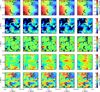 |
Fig. 9. Temporal evolution of a retraction event seen in the retraction simulations. From top to bottom: vertical component of the magnetic field Bz at z2 = −0.60 Mm, temperature at z2, divergence of the velocity ∇ ⋅ v at z2, vertical component of the velocity vz at z2 (vz < 0 are upflows), and the vx component of the velocity at z = z2. The arrows in the first row show the horizontal magnetic field (Bx, By) on the z = z2 plane. The length of the arrows are proportional to |


The second row in Fig. 9 shows the temperature at z = z2 = −0.60 Mm at different times during the evolution of this retraction event. Regions where T(z2) > 5250 K are indicated by white or black contours in the different rows. On the fourth row, vz(z2), the white contours show that enhanced temperatures usually appear close to the downflowing regions in between the sides with opposite-polarity vertical magnetic fields. However, not all downflows present large temperatures. In addition, the black contours in the fifth row, vx(z2), indicate that the regions of enhanced temperature usually appear at the edges of the converging flows along the x-axis. From here we can surmise that the temperature enhancement is due to the plasma being compressed sideways and possibly along the vertical direction as well. This is confirmed in the third row, where we present the values of ∇ ⋅ v at z2 (see also Moll et al. 2012). Here, we can see that large temperatures (black contours) correlate almost perfectly with regions where ∇ ⋅ v < 0. It is therefore possible to state that the terms of the energy equation responsible for the increased temperatures are: −Pg∇ ⋅ v + ν(2)(∇ ⋅ v)2 (Galsgaard & Nordlund 1996). The first of these two terms refers to heating due to mechanical compression or expansion, whereas the second one models the so-called viscous heating Qvisc, with ν(2) being the viscosity coefficient. We can see that in regions where ∇ ⋅ v > 0, both terms compete against each other, whereas in regions where ∇ ⋅ v < 0, both terms contribute to heating. This is the reason why the third row in Fig. 9 shows a much better correlation between regions of enhanced temperature and ∇ ⋅ v < 0.
In order to investigate this further, in Fig. 10 we display the temperature fluctuation with respect to the box average at the same height (left panel), the ratio between vx and the local sound speed cs, the ratio between vz and the local sound speed cs, and ∇ · v, all on the (x, z) plane along the horizontal slice shown in the first column of Fig. 9. The temperature fluctuation (leftmost panel) is positive or negative in regions where the temperature is higher or lower, respectively, than the average temperature at the same height over the entire box. Regions where the temperature fluctuation is greater than 1000 Kelvin are enclosed by the white solid contour in all four panels. This figure shows that the increase in the temperature for z < −0.250 Mm is fueled by a double shock on the horizontal direction (second panel): either side of the white contours, the Mach number (restricted to vx) is higher than one, where in the middle region it drops to very low values. In addition, the values of the density and gas pressure are about 50%–70% larger in the region within the white contours than in the regions outside. This is in agreement with the Rankine-Hugoniot relations, although for this case it would be more adequate to include the effects of the magnetic field (Ferriz-Mas & Moreno-Insertis 1987). As far as the vertical velocities are concerned, we see that slightly above the continuum (black solid lane) at around x ≈ 7 Mm the Mach number restricted to vz (third panel in Fig. 10) is also above 1. This also produces a shock front that heats the atmosphere, but because of the larger densities at this depth, the temperature enhancement is comparatively smaller. The fourth panel clearly indicates that the temperature enhancements above 1000 Kelvin (white contours) closely follow those regions where ∇ · v < 0. This further demonstrates that, as described above, viscous heating through shock dissipation is responsible for the observed temperature enhancements.
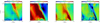 |
Fig. 10. Overview of some physical parameters on the (x, z)-plane along the horizontal cut depicted by the horizontal line at y ≈ 5.3 Mm in the first row of Fig. 9. From left to right: temperature fluctuation with respect to the box-averaged T(z), ratio between vx and the local sound speed cs, ratio between vz and the local sound speed cs, and divergence of the velocity ∇ · v. White contours enclose regions where the temperature fluctuation is greater than 1000 K. The black solid line indicates the location where τR = 1. The horizontal black dashed line is located at z = z2 = −0.60 Mm and therefore corresponds to the height of the plane depicted in Fig. 9. Arrows indicate the velocity field in the (x, z)-plane. |
The description above qualitatively fits the findings by Bellot Rubio (2009), where large horizontal flows were observed and ascribed to the formation of shock fronts. However, a detailed comparison can only be made by calculating synthetic Stokes profiles from the simulations presented here.
It is worth mentioning that in this entire region, we see no sign of magnetic reconnection anywhere, including close to the upper boundary z ≈ −0.60 Mm, even though we used a temporal cadence of 10 s so as to be able to capture fast transient U-loops moving upwards in the atmosphere. In the mixed-polarity simulations, we are also missing the strong vertical upflows that are present in the flux emergence simulations (see Fig. 7; left panel). This is, at first glance, at odds with the results of Cameron et al. (2011), where reconnection events were found in simulations with a similar initial setup. However, after closer inspection, this difference is to be expected, because in our mixed-polarity simulations, the magnetic field lines are supposed to be initially connected when using a potential field upper boundary. To prevent any unwanted transient behaviour before the magnetic field configuration at the top becomes potential (as we start from a purely vertical magnetic-field configuration), we introduced the neutral magnetic stripe in between, so that by the time the opposite polarities meet, the upper boundary field configuration has reached a potential field configuration. For this reason, our setup cannot be directly compared to that of Cameron et al. (2011).
4.2. Reconnection event
Around time t = t0 = 120 min, at location (x, y)≈(3.35,7.35) Mm in the flux-emergence simulation (Sect. 2.2.3), a very conspicuous case of magnetic reconnection takes place close to the upper boundary of the simulation box. The location of this event is highlighted by a white squared box in Figs. 4 and 5. The evolution of the physical parameters during this event (from t0 − 20 s until t0 + 20 s) is shown in Figs. 11 and 12. The first of these two figures shows the physical parameters on the solar surface (x, y) at a height of z2 = −0.60 Mm above τR = 1. The Bx and By components of the magnetic field are also displayed at an additional height of z1 = −0.57 Mm, which is slightly below z2. The second of the aforementioned figures shows the physical parameters on the (x, z) plane for a fixed y = 8.1 Mm. This slice is shown as a white horizontal line on the uppermost panel of Fig. 11. The event starts when the apex of an Ω-loop with Bx < 0 (fourth row in Fig. 12) that lies above a granular cell reaches a region very close to the upper boundary of the box where Bx > 0. This can be seen in the fourth row in Fig. 12 or by comparing the fourth and fifth rows in Fig. 11. Furthermore, by comparing the third (vz(z2)) and fourth (Bx(z1)) rows in Fig. 11, we notice that the loop extends over the entire granular cell in both directions, closely resembling a flux sheet (as seen from above). The magnetic sheet features two footpoints of opposite Bz polarities on either side of the granular cell (fifth row in Fig. 12). The first signs of heating are seen at t = t0 − 10 s at around (x, y)≈(4.1, 8.1) Mm (top panels in Fig. 11) where the temperature suddenly increases by up to 1000–2000 Kelvin at the centre of the granular cell (see third row in this figure). This happens at a location that is closer to the Bz > 0-footpoint of the loop than to the Bz < 0-footpoint. Twenty seconds later, at t = t0 + 10, and (x, y)≈(4.7, 8.1) Mm, the region above the Bz < 0-footpoint also shows signs of heating. After t > t0, we notice an excellent correlation between temperature at z = z2 = −0.60 Mm (first row in Fig. 11) and the square of the horizontal component of the electric currents  (second row). The correlation can also be highlighted by the white and black contours in Fig. 11, which correspond to those regions where T(z2) > 4750 K and
 ![Mathematical equation: $ \log[j_\perp^2(z_2)] > -2.0 $](/articles/aa/full_html/2023/05/aa45701-22/aa45701-22-eq7.gif) (with j⊥ given in A m−2), respectively. This correlation is very suggestive of magnetic reconnection. Closer inspection of j⊥ indicates that jx > jy, although the latter is still significant. During the event, jz (not shown) is about 1–2 orders of magnitude smaller than the horizontal components of the electric current density within the white and black contours. The dominant contributions to jx and jy are, respectively, ∂By/∂z and ∂Bx/∂z, indicating that reconnection occurs due to horizontal fields changing their orientation along the vertical, which finally leads to reconnection. This can be further understood when looking at the orientation of the horizontal magnetic field at z = z1 over time, as indicated by white arrows in Fig. 11 (fourth to seventh rows). If we focus on the central point of (x, y) = (4.1, 8.1) Mm at t0 − 20 s, the magnetic field at z = z2 (fifth and seventh rows) is mostly oriented along the 12 o’clock direction, while at t0 − 10 s it has changed its orientation to 10 o’clock because of the rise from underneath of a flux-sheet orientated along the x-direction. At the same coordinates, a temperature enhancement and a large upflow (vz(z2)) on the third row are located; these develop further over time.
(with j⊥ given in A m−2), respectively. This correlation is very suggestive of magnetic reconnection. Closer inspection of j⊥ indicates that jx > jy, although the latter is still significant. During the event, jz (not shown) is about 1–2 orders of magnitude smaller than the horizontal components of the electric current density within the white and black contours. The dominant contributions to jx and jy are, respectively, ∂By/∂z and ∂Bx/∂z, indicating that reconnection occurs due to horizontal fields changing their orientation along the vertical, which finally leads to reconnection. This can be further understood when looking at the orientation of the horizontal magnetic field at z = z1 over time, as indicated by white arrows in Fig. 11 (fourth to seventh rows). If we focus on the central point of (x, y) = (4.1, 8.1) Mm at t0 − 20 s, the magnetic field at z = z2 (fifth and seventh rows) is mostly oriented along the 12 o’clock direction, while at t0 − 10 s it has changed its orientation to 10 o’clock because of the rise from underneath of a flux-sheet orientated along the x-direction. At the same coordinates, a temperature enhancement and a large upflow (vz(z2)) on the third row are located; these develop further over time.
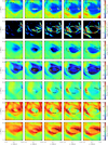 |
Fig. 11. Temporal evolution of the physical parameters during a reconnection event seen in the flux-emergence simulations. Values are given on the solar surface (x, y) at two different heights: z1 = −0.57 Mm and z2 = −0.60 Mm, with z2 being closer to the upper boundary of the simulation box. The location of the reconnection event is indicated by the squared box in Figs. 4 and 5. From top to bottom: T(x, y, z2), logarithm of the square of the horizontal component of the electric current |


![Mathematical equation: $ \log[j^2_\perp(z_2)] > -2.0 $](/articles/aa/full_html/2023/05/aa45701-22/aa45701-22-eq10.gif)
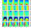 |
Fig. 12. Temporal evolution of the physical parameters on the (x, z) plane for the slice indicated by the white line (y = y1) in the upper panels of Fig. 11. From top to bottom: temperature difference with respect to the box average at each height, vx(x, y1, z), vz(x, y1, z), Bx(x, y1, z), Bz(x, y1, z). The arrow field represents the direction of the velocity in the second and third rows and the magnetic field in the fourth and fifth rows, on the (x, z) plane. The length of the arrows is proportional to |


Examples of emergence of flux-sheet-like structures on granular cells have been found before in both simulations (Moreno-Insertis et al. 2018) and observations (Fischer et al. 2019). Moreover, observationally it was already established that the rise of such flux sheets or Ω-loops might be linked to magnetic reconnection and supersonic upflows in the upper photosphere (Borrero et al. 2010, 2013). Interestingly, the topology of the magnetic field during the reconnection event in these simulations is rather different from other commonly observed events where opposite Bz polarities meet horizontally (Yang et al. 2009).
It is worth mentioning that, from an observational point of view, the magnetic field is normally inferred in iso-surfaces of optical depth (e.g. τR = 10−4). Had we calculated electric currents from those, we would have inferred very different values of j. This happens because the increased temperature and gas pressure at the reconnection region leads to a very large opacity in those layers and therefore to a very warped optical-depth isosurface. This would give the false impression that the most important terms contributing to the electric currents are ∂Bx/∂y and ∂By/∂x. Therefore, it is very important that the inference of the electric currents is done by calculating spatial derivatives in the Cartesian domain. From an observational point of view, this is now possible thanks to newly developed Stokes inversion techniques (Pastor Yabar et al. 2019, 2021).
Within the region enclosed by the white contours (at all five time steps in Fig. 11), we find that the average angle between B and j is 67°, with a standard deviation of 17°. In this same region, the average plasma-β = 2.9 with a standard deviation of 2.1. These values are in qualitative agreement with two-dimensional models where reconnection occurring at locations characterised by β > 1 are also characterised by j ⊥ B (see Sect. 1.11 in Spruit 2013). The fact that the magnetic field and electric current density are not entirely perpendicular is an effect of having an additional component of the magnetic field that can be constant across the current sheet (see Sect. 5.8 of Jackson 1975).
The temporal evolution of the Bx(x, z) (fourth row in Fig. 12) clearly indicates that the Ω-loop or flux sheet is rising in time. This is further demonstrated by the upflowing velocities (vz(x, z) < 0 on the third row of Fig. 12) and by the fact that the arms of the loop are moving away from each other at all photospheric heights (see vx(x, z) on the second row). The situation described here is exactly the opposite to the case of loop retraction, where the footpoints move towards each other at all heights and a downflow is present in between (see Sect. 4.1 and Fig. 10). Figure 12 shows that, at the time and place where the first clear signs of heating appear, t = t0 − 10 and (x, z)≈(4.1, −0.60) Mm, a large surge in the upflow velocity of up to 12–15 km s−1 develops (see third row). These large upflows fade quickly afterwards even though heating still continues (compare first and third rows in Fig. 11). Large upflows and heating in the upper photosphere caused by reconnection are ubiquitous in the flux-emergence simulation (Sect. 2.2.3) as seen by the large tail of vz < −10 km s−1 in Fig. 7, as well as in the long tail of T > 7000 K in Fig. 8 (dashed black lines for τR = 2 × 10⁻³).
Although it is clear that this event is caused by magnetic reconnection, we still need to determine the physical mechanism responsible for the heating that ensues. At first glace (second row in Fig. 11), the spatial correlation between enhanced temperatures and electric currents might lead us to conclude that the heating is being caused by the dissipation of electric currents (i.e. Joule heating). In order to investigate this further, we turn our attention to Fig. 13, where we display a close-up view of the physical parameters in the upper atmosphere (z ∈ [ − 0.46, −0.60] Mm) as a function of time. Above z = −0.60 Mm, the currents quickly drop to zero because of the potential upper boundary condition. As can be seen on the second row, the Joule heating term, Qjoule = j2/σ, is largest close to the upper boundary. More specifically, it is largest at t0 − 10 s, where the first signatures of heating appear close to the loop apex at (x, z)≈(4.1, −0.6) Mm. At this location, the plasma is expanding upwards and therefore the expansion/compression term contributes to cooling (third row; −Pg∇ ⋅ v < 0). However, the cooling due to expansion is an order of magnitude lower than the heating produced by current dissipation. As time progresses, Qjoule decreases, although it remains significant at the loop apex. In spite of this, no further signatures of heating are seen at the apex. This is possibly due to the large upflow velocities of vz < −10 km s−1 combined with the time step of 10 s between snapshots: any further heating at the loop apex is quickly advected upwards and outside of the upper boundary. This suggests that in order to fully capture reconnection events, an even higher cadence might be needed for the output data (Sect. 2.2.1).
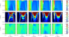 |
Fig. 13. Similar to Fig. 12 but focusing only on the upper atmosphere: z ∈ [ − 0.46, −0.60] Mm and showing (from top to bottom) the temperature difference with respect to the box average at each height, Joule heating Qjoule, and heating and cooling due to compression or expansion −Pg∇ ⋅ v, respectively. |
Interestingly, for t > t0, we see enhanced temperatures on the arms of the loops that move away from each other (regions of large positive or negative vx; second row in Fig. 12) as the magnetic loop opens up and the field lines become more vertical. In these regions, the terms Qjoule = j2/σ decreases with respect to its values at the loop apex. At the same time, the term −Pg∇ ⋅ v becomes more positive, indicating that the horizontal compression of the plasma also contributes to the heating in the arms of the loop, at least partially. Indeed, the Joule heating term still dominates over the compression term. However, we have to keep in mind that for reasons of numerical stability, at least locally, unrealistically high hyperdiffusivity values are applied in the STAGGER code. As a consequence, in the present simulations, the electrical conductivity σ is artificially lower compared to the real Sun, leading to an enhanced contribution from Joule heating. Therefore, it remains unclear as to whether on the real Sun, the main contribution to photospheric heating during reconnection events comes from Joule heating or from compression. For this reason, it would be interesting to repeat these experiments with different values of magnetic diffusivity, but this lies beyond the scope of the present work. We also note that the sideways flows on either side of the apex of the loop turn down along its arms towards the footpoints at (x, z)≈(3.5, 0.0) Mm and (x, z)≈(4.8, 0.0) Mm (third row). Consequently, the downflows surrounding the granule become stronger and wider as time passes (not shown here).
Overall, this entire reconnection event lasts for less than a minute. This is much shorter than similar events seen in other simulations (Cameron et al. 2011; Danilovic 2017) where reconnection occurs on timescales of several minutes. However, the duration of the event is related to the amount of available magnetic flux and the magnetic field configuration, which are not the same in the different simulations.
5. Summary and conclusions
In this paper, we address the question of whether or not it is possible to distinguish between the photospheric signatures of the two main magnetic-flux-removal processes present in the quiet Sun: retraction and reconnection. To this end, we employed 3D MHD non-grey radiative simulations performed with the STAGGER code with two types of initial magnetic field configurations: (a) mixed-polarity simulations with a potential magnetic field at the upper boundary (Sect. 2.2.1) where we theoretically expect the retraction process to be dominant; and (b) magnetic flux emergence simulations (Sect. 2.2.3), where we expect reconnection to occur. Our expectations are confirmed by a detailed statistical analysis of the simulation results as well as an in-depth study of two particular retraction and reconnection events: whereas (a) is dominated by the retraction of Ω-loops back below the surface (Fig. 10); (b) is mostly characterised by reconnection events (i.e. nanoflare-like) leading to temperature enhancements in the vicinity of current sheets due to Ohmic heating, as well as diverging velocities leading to compressional heating (Fig. 12).
In the case of retraction, as Fig. 7 (solid blue and solid cyan) shows, for the ‖Bz,init‖ = 1000 G mixed-polarity simulation, we do see pronounced downflow velocities at the flux-removal sites (below the apexes of the loops), along with enhanced horizontal converging inflows between the loop footpoints. We also observe increased temperatures due to shock dissipation, as the converging inflows surpass Mach one and suddenly drop below Mach one when they collide with each other at the centre of the retracting loop (see Fig. 10). Retraction signatures are more pronounced for the stronger initial field of ‖Bz,init‖ = 1000 G than with ‖Bz,init‖ = 200 G (compare to Figs. B.1 and B.2). This is further supported by the histograms in Figs. 7 and 8, which show the statistical properties of the mixed-polarity runs compared to the single-polarity reference runs (Sect. 2.2.1). These histograms also demonstrate that the mixed-polarity field simulations show supersonic vertical downflows but no comparable upflows. Overall, the results from the retraction setup simulations are in agreement with the results of Thaler & Spruit (2017).
In the case of flux emergence, we see enhanced temperatures in the upper photospheric layers (black dashed on the left panel in Fig. 8) at locations where large electric currents are also present (Fig. 11). This is highly suggestive of reconnection taking place as the apexes of rising Ω-loops reach the upper photosphere where they meet a magnetic field of opposite horizontal polarity (i.e. Bx < 0 and Bx > 0; Fig. 12). At the time and place where reconnection occurs, we also detect supersonic upflow velocities mostly in the upper photospheric layers (see black dashed lines in the left panel of Fig. 7). These simulations also feature large horizontal velocities (black dashed lines in the right panel of the same figure) that compress the plasma sideways, thereby heating it. As in the retraction setup, these large horizontal velocities are due to retraction of magnetic field lines. However, unlike the retraction setup, where these horizontal velocities are converging, in the flux-emergence setup they are diverging because they are caused by the sideways retraction of magnetic field lines that occurs after reconnection.
Acknowledgments
A huge thanks for the very helpful discussions with and comments from Prof. H. Spruit which lead to a substantial improvement of our understanding and the paper. This work has made use of NASA/ADS abstract service.
References
- Beeck, B., Collet, R., Steffen, M., et al. 2012, A&A, 539, A121 [NASA ADS] [CrossRef] [EDP Sciences] [Google Scholar]
- Bellot Rubio, L. R. 2009, ApJ, 700, 284 [NASA ADS] [CrossRef] [Google Scholar]
- Borrero, J. M., Martínez-Pillet, V., Schlichenmaier, R., et al. 2010, ApJ, 723, L144 [NASA ADS] [CrossRef] [Google Scholar]
- Borrero, J. M., Martínez Pillet, V., Schmidt, W., et al. 2013, ApJ, 768, 69 [Google Scholar]
- Cameron, R., Vögler, A., & Schüssler, M. 2011, A&A, 533, A86 [NASA ADS] [CrossRef] [EDP Sciences] [Google Scholar]
- Cheung, M. C. M., Schüssler, M., & Moreno-Insertis, F. 2007, A&A, 461, 1163 [NASA ADS] [CrossRef] [EDP Sciences] [Google Scholar]
- Danilovic, S. 2017, A&A, 601, A122 [NASA ADS] [CrossRef] [EDP Sciences] [Google Scholar]
- Ferriz-Mas, A., & Moreno-Insertis, F. 1987, A&A, 179, 268 [NASA ADS] [Google Scholar]
- Fischer, C. E., Borrero, J. M., Bello González, N., & Kaithakkal, A. J. 2019, A&A, 622, L12 [NASA ADS] [CrossRef] [EDP Sciences] [Google Scholar]
- Galsgaard, K., & Nordlund, Å. 1996, J. Geophys. Res., 101, 13445 [NASA ADS] [CrossRef] [Google Scholar]
- Gustafsson, B. 1973, Uppsala Astron. Obs. Ann., 5 [Google Scholar]
- Gustafsson, B., Bell, R. A., Eriksson, K., & Nordlund, A. 1975, A&A, 500, 67 [NASA ADS] [Google Scholar]
- Hathaway, D. H. 2015, Liv. Rev. Sol. Phys., 12, 4 [Google Scholar]
- Howard, R., & Labonte, B. J. 1981, Sol. Phys., 74, 131 [NASA ADS] [CrossRef] [Google Scholar]
- Jackson, J. D. 1975, Classical Electrodynamics (New York: Wiley) [Google Scholar]
- Moll, R., Cameron, R. H., & Schüssler, M. 2012, A&A, 541, A68 [NASA ADS] [CrossRef] [EDP Sciences] [Google Scholar]
- Moreno-Insertis, F., Martinez-Sykora, J., Hansteen, V. H., & Muñoz, D. 2018, ApJ, 859, L26 [Google Scholar]
- Nordlund, A. 1982, A&A, 107, 1 [Google Scholar]
- Nordlund, Å., & Stein, R. F. 1990, Comput. Phys. Commun., 59, 119 [NASA ADS] [CrossRef] [Google Scholar]
- Nordlund, Å., Stein, R. F., & Asplund, M. 2009, Liv. Rev. Sol. Phys., 6, 2 [Google Scholar]
- Pastor Yabar, A., Borrero, J. M., & Ruiz Cobo, B. 2019, A&A, 629, A24 [NASA ADS] [CrossRef] [EDP Sciences] [Google Scholar]
- Pastor Yabar, A., Borrero, J. M., Quintero Noda, C., & Ruiz Cobo, B. 2021, A&A, 656, L20 [NASA ADS] [CrossRef] [EDP Sciences] [Google Scholar]
- Pontin, D. I., & Priest, E. R. 2022, Liv. Rev. Sol. Phys., 19, 1 [NASA ADS] [CrossRef] [Google Scholar]
- Priest, E. R., & Syntelis, P. 2021, A&A, 647, A31 [EDP Sciences] [Google Scholar]
- Priest, E. R., Chitta, L. P., & Syntelis, P. 2018, ApJ, 862, L24 [Google Scholar]
- Solanki, S. K., Barthol, P., Danilovic, S., et al. 2010, ApJ, 723, L127 [NASA ADS] [CrossRef] [Google Scholar]
- Spruit, H. C. 2013, ArXiv e-prints [arXiv:1301.5572] [Google Scholar]
- Stein, R. F., & Nordlund, Å. 1998, ApJ, 499, 914 [Google Scholar]
- Thaler, I., & Spruit, H. 2017, A&A, 601 [Google Scholar]
- Yang, S., Zhang, J., & Borrero, J. M. 2009, ApJ, 703, 1012 [NASA ADS] [CrossRef] [Google Scholar]
- Zwaan, C. 1987, ARA&A, 25, 83 [NASA ADS] [CrossRef] [Google Scholar]
Appendix A: Initial states
The following figures show the physical parameters of a typical hydrodynamic snapshot used for an initial setup.
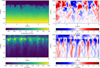 |
Fig. A.1. Physical quantities averaged along the y-direction for an example hydrodynamical snapshot: temperature [104K], velocity in x-direction [km/s], horizontal velocity in [km/s], vertical velocity in [km/s]. |
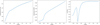 |
Fig. A.2. Horizontally averaged quantities from an example hydrodynamical snapshot: natural logarithm of density in [g cm-3], temperature [104K], vertical velocity in [km/s]. |
Appendix B: Mixed-polarity setup with ‖Bz,init‖ = 200 G.
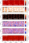 |
Fig. B.1. Temporal evolution of the physical parameters at τR = 1 in the ‖Bz,init‖ = 200 G mixed-polarity setup (Sect. 2.2.1). From top to bottom: Bz, |
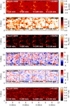 |
Fig. B.2. Temporal evolution of the physical parameters at τR = 2 × 10⁻³ in the ‖Bz,init‖ = 200 G mixed-polarity setup (Sect. 2.2.1). From top to bottom: Bz, |

All Figures
|
Fig. 1. Natural logarithm of magnetic energy integrated over the whole simulation box and normalised to the initial magnetic energy value for each simulation. The mixed-polarity simulation with ‖Bz,init‖ = 200 G is shown in blue, whereas green shows ‖Bz,init‖ = 1000 G. The flux emergence simulation is depicted in red. |
| In the text | |
|
Fig. 2. Temporal evolution of the physical parameters at τR = 1 in the ‖Bz,init‖ = 1000 G mixed-polarity setup (Sect. 2.2.1). From top to bottom: Bz, |
| In the text | |
|
Fig. 3. Same as Fig. 2 but at τR = 2 × 10⁻³ (i.e. higher up in the photosphere and closer to the upper boundary). |
| In the text | |
|
Fig. 4. Temporal evolution of the physical parameters at τR = 1 in the flux-emergence setup (Sect. 2.2.3). From top to bottom: Bz, |
| In the text | |
|
Fig. 5. Same as Fig. 4 but at τR = 2 × 10⁻³ (i.e. higher up in the photosphere and closer to the upper boundary). |
| In the text | |
|
Fig. 6. Temporal evolution of the absolute value of the magnetic field |Btot| for the flux-cancelling event described in Sect. 2.2.3 in the flux-emergence setup at τR = 2 × 10⁻³. |
| In the text | |
|
Fig. 7. Probability distributions of the vertical velocity vz (left panel) and the horizontal velocity |
| In the text | |
|
Fig. 8. Probability distributions of the temperature (left panel) and the horizontal magnetic field Bh (right panel). Results for the mixed-polarity and single-polarity runs (Sect. 2.2.3) with ‖Bz,init‖ = 1000 G are shown in solid cyan and dashed cyan for τR = 1 and solid blue and dashed blue for τR = 2 × 10⁻³, respectively, whereas results for the run with ‖Bz,init‖ = 200 G are indicated in solid emerald green and dashed emerald green for τR = 1 and solid green and dashed green for τR = 2 × 10⁻³, respectively. The flux-emergence simulation results are shown in black for τR = 1 (solid) and τR = 2 × 10⁻³ (dashed). |
| In the text | |
|
Fig. 9. Temporal evolution of a retraction event seen in the retraction simulations. From top to bottom: vertical component of the magnetic field Bz at z2 = −0.60 Mm, temperature at z2, divergence of the velocity ∇ ⋅ v at z2, vertical component of the velocity vz at z2 (vz < 0 are upflows), and the vx component of the velocity at z = z2. The arrows in the first row show the horizontal magnetic field (Bx, By) on the z = z2 plane. The length of the arrows are proportional to |
| In the text | |
|
Fig. 10. Overview of some physical parameters on the (x, z)-plane along the horizontal cut depicted by the horizontal line at y ≈ 5.3 Mm in the first row of Fig. 9. From left to right: temperature fluctuation with respect to the box-averaged T(z), ratio between vx and the local sound speed cs, ratio between vz and the local sound speed cs, and divergence of the velocity ∇ · v. White contours enclose regions where the temperature fluctuation is greater than 1000 K. The black solid line indicates the location where τR = 1. The horizontal black dashed line is located at z = z2 = −0.60 Mm and therefore corresponds to the height of the plane depicted in Fig. 9. Arrows indicate the velocity field in the (x, z)-plane. |
| In the text | |
|
Fig. 11. Temporal evolution of the physical parameters during a reconnection event seen in the flux-emergence simulations. Values are given on the solar surface (x, y) at two different heights: z1 = −0.57 Mm and z2 = −0.60 Mm, with z2 being closer to the upper boundary of the simulation box. The location of the reconnection event is indicated by the squared box in Figs. 4 and 5. From top to bottom: T(x, y, z2), logarithm of the square of the horizontal component of the electric current |
| In the text | |
|
Fig. 12. Temporal evolution of the physical parameters on the (x, z) plane for the slice indicated by the white line (y = y1) in the upper panels of Fig. 11. From top to bottom: temperature difference with respect to the box average at each height, vx(x, y1, z), vz(x, y1, z), Bx(x, y1, z), Bz(x, y1, z). The arrow field represents the direction of the velocity in the second and third rows and the magnetic field in the fourth and fifth rows, on the (x, z) plane. The length of the arrows is proportional to |
| In the text | |
|
Fig. 13. Similar to Fig. 12 but focusing only on the upper atmosphere: z ∈ [ − 0.46, −0.60] Mm and showing (from top to bottom) the temperature difference with respect to the box average at each height, Joule heating Qjoule, and heating and cooling due to compression or expansion −Pg∇ ⋅ v, respectively. |
| In the text | |
|
Fig. A.1. Physical quantities averaged along the y-direction for an example hydrodynamical snapshot: temperature [104K], velocity in x-direction [km/s], horizontal velocity in [km/s], vertical velocity in [km/s]. |
| In the text | |
|
Fig. A.2. Horizontally averaged quantities from an example hydrodynamical snapshot: natural logarithm of density in [g cm-3], temperature [104K], vertical velocity in [km/s]. |
| In the text | |
|
Fig. B.1. Temporal evolution of the physical parameters at τR = 1 in the ‖Bz,init‖ = 200 G mixed-polarity setup (Sect. 2.2.1). From top to bottom: Bz, |
| In the text | |
|
Fig. B.2. Temporal evolution of the physical parameters at τR = 2 × 10⁻³ in the ‖Bz,init‖ = 200 G mixed-polarity setup (Sect. 2.2.1). From top to bottom: Bz, |
| In the text | |
Current usage metrics show cumulative count of Article Views (full-text article views including HTML views, PDF and ePub downloads, according to the available data) and Abstracts Views on Vision4Press platform.
Data correspond to usage on the plateform after 2015. The current usage metrics is available 48-96 hours after online publication and is updated daily on week days.
Initial download of the metrics may take a while.