| Issue |
A&A
Volume 671, March 2023
|
|
|---|---|---|
| Article Number | A63 | |
| Number of page(s) | 13 | |
| Section | The Sun and the Heliosphere | |
| DOI | https://doi.org/10.1051/0004-6361/202245500 | |
| Published online | 06 March 2023 | |
Detailed composition of iron ions in interplanetary coronal mass ejections based on a multipopulation approach⋆
1
Institute of Experimental and Applied Physics (IEAP), University of Kiel, Leibnizstrasse 11, 24118 Kiel, Germany
e-mail: chaorangu@physik.uni-kiel.de
2
School of Geophysics and Information Technology, China University of Geosciences (Beijing), Beijing 100083, PR China
Received:
18
November
2022
Accepted:
13
January
2023
Context. Coronal mass ejections (CMEs) are extremely dynamical, large-scale events in which plasma – but not only the coronal plasma – is ejected into interplanetary space. If a CME is detected in situ by a spacecraft located in the interplanetary medium, it is then called an interplanetary coronal mass ejection (ICME). This solar activity has been studied widely since coronagraphs were first flown into space in the early 1970s.
Aims. Charge states of heavy ions reflect important information about the coronal temperature profile due to the freeze-in effect and it is estimated that iron ions freeze in at heights of ∼5 solar radii. However, the measured charge-state distribution of iron ions cannot be composed of only one single group of plasma. To identify the different populations of iron charge-state composition of ICMEs and determine their sources, we developed a model that independently uses two, three, and four populations of iron ions to fit the measured charge-state distribution in ICMEs detected by the Advanced Composition Explorer (ACE) at 1 AU.
Methods. Three parameters are used to identify a certain population, namely freeze-in temperature, relative abundance, and kappa value (κ), which together describe the potential non-Maxwellian kappa distributions of coronal electrons. Our method chooses the reduced chi-squared to describe the goodness of fit of the model to the observations. The parameters of our model are optimized with the covariance-matrix-adaptation evolution strategy (CMA-ES).
Results. Two major types of ICMEs are identified according to the existence of hot material, and both, that is, the cool type and the hot type, have two main subtypes. Different populations in those types have their own features related to freeze-in temperature and κ. The electron velocity distribution function usually contains a significant hot tail in typical coronal material and hot material, while the Maxwellian distribution appears more frequently in mid-temperature material. Our model is also suitable for all types of solar wind and the existence of hot populations as well as the change of temperatures of individual populations may indicate boundaries between ICMEs and individual solar wind streams.
Key words: Sun: coronal mass ejections (CMEs)
Table A.1 is only available at the CDS via anonymous ftp to cdsarc.cds.unistra.fr (130.79.128.5) or via https://cdsarc.cds.unistra.fr/viz-bin/cat/J/A+A/671/A63
© The Authors 2023
 Open Access article, published by EDP Sciences, under the terms of the Creative Commons Attribution License (https://creativecommons.org/licenses/by/4.0), which permits unrestricted use, distribution, and reproduction in any medium, provided the original work is properly cited.
This article is published in open access under the Subscribe to Open model. Subscribe to A&A to support open access publication.
1. Introduction
Coronal mass ejections (CMEs) are extremely dynamical, large-scale solar eruptions. These phenomena were observed directly after corona-graphs were first flown into space in the early 1970s (Tousey 1973; Gosling et al. 1974). The interplanetary counterparts of CMEs measured in situ are interplanetary coronal mass ejections (ICMEs) and are considered to be multidimensional, multiparameter, and multiscale (Wimmer-Schweingruber 2006). Heavy ions, whose nuclei are heavier than helium, are noticeably enhanced in ICMEs compared to solar wind (Bame et al. 1979; Bochsler et al. 1986). One of the signatures of heavy ions in ICMEs is that the average charge states are usually higher than those in the solar wind, which indicates a stronger heating process in the initiation of CMEs (Wimmer-Schweingruber et al. 2006; Gruesbeck et al. 2011; Henke et al. 2001). Meanwhile, unusually low charge states of heavy ions in ICMEs have also been reported (Lepri & Zurbuchen 2010; Song et al. 2017; Feng et al. 2018), which are thought to be possibly related to the cold prominence plasma.
When a CME erupts and propagates outward, the electron density decreases rapidly with solar distance. As the ionization and recombination rates are functions of the electron density (Landi et al. 2012; Dere et al. 1997), charge states of heavy ions will freeze in when the expansion timescale is approximately equal to the recombination timescale at 1–5 solar radii (Geiss et al. 1995; Lepri et al. 2012; Kocher et al. 2017). As a result, the heavy ions in ICMEs measured at 1 AU carry important information about the CME source region (Gruesbeck et al. 2011; Rivera et al. 2019; Kocher et al. 2018; Rodkin et al. 2017).
Iron ions are suitable for investigating detailed compositions of ICME plasma because of their wide range of measured charge states from Fe6+ to Fe20+. Iron ions can also be accurately identified by the Solar Wind Ion Composition Spectrometer (SWICS; Gloeckler et al. 1998) on board the Advanced Composition Explorer (ACE).
With data from ACE, Song et al. (2016) conducted a statistical study of the average charge state of iron ions inside 96 magnetic clouds during solar cycle 23 and classified them into four groups according to a time series of averaged iron charge state. Among the four groups, these authors reported a bimodal distribution with both peaks being higher than 12+ as well as a unimodal distribution with its peak being higher than 12+. The authors also reported two other kinds of distributions of iron average charge state, which remain higher or lower than 12+ throughout the passage of ACE through the magnetic cloud. The spatial variations of the mean charge state of iron ions are explained as the combination of hot and cold plasma layers in ICMEs, as in the layers of an onion (Song & Yao 2020).
A similar scenario, describing the multicomponent and multitemperature structure of CMEs, was reported in a case study by Cheng et al. (2011) based on observations by the Solar Dynamics Observatory (SDO). Hot plasma is frequently observed wrapped around the flux rope (Zhang et al. 2012). The proportion of the hot flux rope configuration occurring in solar eruptions is 49% (Nindos et al. 2015). The enhanced ions with higher charge states are supposed to be heated by an associated flare in the lower corona (Lynch et al. 2011). Ions with normal charge states are possibly related to the current sheet (Song et al. 2016), while those with lower charge states may originate from the cool leading edge (Cheng et al. 2011).
In their case study, Rivera et al. (2019) found that ion distributions in an ICME can be effectively reconstructed using a combination of ions generated within four distinct plasma components (PCs) traveling together but with different thermodynamic histories for C, O, and Fe. Furthermore, the normalized proportions of the four components for iron ions are: 0.10PC1 + 0.33PC2 + 0.33PC3 + 0.24PC4. According to the range of ionic temperature, these authors propose that PC1 originates from prominence, PC2 is the common coronal plasma, and PC3 and PC4 are from the prominence–corona transition region.
According to the average charge-state distribution of iron ions measured by ACE, Gu et al. (2020) divided the 274 ICMEs into three types: Fe1, Fe2, and Fe3. These correspond to three distinct charge-state distribution patterns including a bimodal distribution and two single-peak distributions with their peaks located in a low charge state (Fe9+ or Fe10+) and Fe16+, respectively. The cause of the three different charge-state distribution patterns is unclear. The occurrence rates of the three types of charge-state distributions and the averaged charge states of iron ions in ICMEs are highly related to the solar activity cycle.
However, the specific composition of iron ions in ICMEs, especially for those with a bimodal charge-state distribution, together with the potential source components of iron ions are still unknown. This motivates a study of the composition of plasma in different ICMEs in order to decipher whether or not these are the same, and also whether or not there is a common model of thermal composition for CMEs.
The CHIANTI database makes the assumption of a Maxwellian distribution for the electron velocity distribution function, which is known to not be the appropriate choice for the solar corona and the solar wind (Marsch 2006). Meanwhile, although κ distributions were detected in solar flares, active regions, the transition region, and the solar wind, they have not yet been found in the outer solar corona despite numerous diagnostic attempts (Dzifčáková et al. 2015; Lörinčík et al. 2020; Del Zanna et al. 2022). Charge-state distributions of heavy ions depend on the electron distribution at different freeze-in heights, and so it is important to add κ as a free parameter to our model. Using the CHIANTI database, we make an assumption that the electron distribution in the corona is in ionization equilibrium.
In this work, we study 310 ICMEs from 1998 to 2011 in order to investigate the detailed composition of iron ions in ICMEs. The data and methods are described in Sect. 2. The results are shown in Sect. 3. The discussion is given in Sect. 4, followed by the conclusion in Sect. 5.
2. Data and methods
In this section, we first introduce the data source of the studied ICMEs and the ionization equilibrium data. We then provide details of the model as well as the optimization method incorporated into it. After that, we briefly present the model results and several tests are also presented to show the reliability of those model results.
2.1. The studied ICMEs and the ionization equilibrium data
This work uses the charge-state distributions of iron ions measured at 1 AU by ACE/SWICS (Gloeckler et al. 1998) from 1998 to 2011. The data are published with a cadence of 2 h. All the data are provided by the ACE Science Center1.
The ICMEs studied in this work are listed by Cane & Richardson (2003) and Richardson & Cane (2010), and by the ACE Science Center2 (known as R&C list). From February 1998 to August 2011, 310 ICMEs are selected (from 319 cases in total; 9 cases with data gaps are removed) to be applied to our model; their charge-state distributions of iron ions were recorded by ACE/SWICS (Gloeckler et al. 1998; Geiss et al. 1995). To identify individual ICMEs, we added the case number to all the 310 ICMEs. The start time of each ICME is from the original list at the ACE Science Center. For each ICME, we averaged the charge-state distribution of iron ions, which means one averaged distribution corresponds to one recorded ICME, and the error is set to be the maximum statistical uncertainty throughout the whole period.
In this work, the ionization equilibrium data for Fe under different κ is from the CHIANTI-Kappa database (a package for synthesis of optically thin spectra for the non-Maxwellian kappa-distributions based on the CHIANTI database, version 10.0.1; Dzifčáková et al. 2015, 2021). Pearson correlation analysis, Spearman correlation analysis, and kernel density estimation (KDE) are also applied in the analysis of the results of our model.
2.2. Multipopulation model
For convenience, we use the following abbreviations and notations:
In our model, the measured charge-state distribution of iron ions is assumed to be a combination of n populations of plasma. Each population has its own freeze-in temperature and relative abundance. Here, we made an assumption that the corresponding plasma at a certain freeze-in height is in charge-state equilibrium. As the outer solar corona and solar wind are not in thermal equilibrium and their particle velocity distributions exhibit supra-thermal tails (Dudík et al. 2017), κ becomes an additional dimension when we identify a specific population of iron ions.
Here, f(Ti, κi) represents the charge-state distribution of a group of iron ions that freeze in at temperature Ti [log(T/K)] with a certain electron distribution condition controlled by κi. Our two-population, three-population, and four-population models correspond to n = 2, 3, 4. Here, f(Ti, κi) is based on the CHIANTI-kappa database (Dzifčáková et al. 2015, 2021).
The allowed temperature range for all populations is the same, from 104.5 to 108.5 K, and is converted to logarithmic coordinates. In our model, κ ∈ [1.55, 33]. Both of the boundary values are given by the CHIANTI-kappa database and the kappa distribution is very close to a Maxwellian distribution if κ = 33.
2.3. Objective function and optimization
For each model, we calculate  to test the goodness-of-fit and this is defined as the chi-square per degree of freedom:

where χ2 is a weighted sum of squared deviations:
Here, Oic and Eic are from the ACE Science Center. The degree of freedom v equals the number of observations N minus the number of fitted parameters m. In this work, we have 15 charge states available (N = 15) and m depends on the number of populations in the model. Our objective function ϕ is defined through  :
:
where x is the solution determined by all fitted parameters. Taking the four-population model as an example, there are 11 fitted parameters in total, which gives x = (T1, T2, T3, T4, Arel, 1, Arel, 2, Arel, 3, κ1, κ2, κ3, κ4)⊺. Here, Arel, 4 is given by Arel, 4 = 1 − Arel, 1 − Arel, 2 − Arel, 3. In that case, our optimization is actually searching for the best solution, which represents the smallest  , in an eleven-dimensional space. We accept over-fitting situations where ϕ(x) < 1. The cause of over-fitting is investigated in Sect. 2.5. We use the covariance-matrix-adaptation evolution strategy (CMA-ES) to find the target global optimum.
The CMA-ES is a stochastic method for real-parameter (continuous domain) optimization of nonlinear, nonconvex functions (Hansen 2016). In our model, the boundaries of every dimension in the solution space have been renormalized and the allowed value ranges mentioned in Sect. 2.2 are all mapped to [0, 100]. After the optimization, parameters would be mapped to their original value ranges. Take the four-population model as an example, the initial input solution x would then be (50, 50, 50, 50, 25, 25, 25, 50, 50, 50, 50)⊺ (50 here represents the medium value of T or κ) and the initial step size set to 20. Other parameters are set to their default values. To those solutions with more than one parameter out of its range, the objective function value would be set to a large value (110 000 for the four-population model) plus the square of the distance between the initial input solution and the current solution in the whole solution space, meaning that the direction of the evolutionary path would be altered to avoid further progress in the direction that would result in out-of-range parameters.
For the studied model results in this work, we performed ten runs for each ICME. Here, one run means that the two-population, three-population, and four-population models would be carried out independently once and the optimal solution would be retained as the final result of this run. The source code for the CMA-ES (version 3.2.1) applied in this work was written using Python 3.8.8.
2.4. Majority population
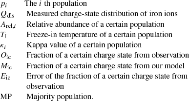
Four cases have been selected as examples to illustrate the model results in Fig. 1. Contributions of different populations in the model are clearly visible in Fig. 1 and some populations only occupy a very limited share of the whole ICME plasma, such as p4 in Fig. 1b, and more can be found in the appendix.
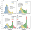 |
Fig. 1. Measured and modeled charge-state distributions of iron ions of four selected ICMEs. The case numbers of the four ICMEs are marked in each subplot and detailed parameters of populations are given in the form of pn(T, Arel, κ). All distributions are normalized to their respective sum and the error bars indicate the observational uncertainty. |
These populations, which represent only a small fraction of the complete charge state distribution, sometimes have extremely high or low freeze-in temperatures. These populations are therefore more likely to be optimization artifacts than a physically meaningful result.
Therefore, we define a proportion threshold to assure the reliability of the parameters of the populations given by our model. The threshold is set to 10%, which is derived from the typical statistical error and fits the peak value of the histogram of the sums of the statistical uncertainty of each case very well. Any individual population with less influence on the overall charge state distribution than the observational error is considered unreliable. Only if a population occupies at least 10% can it significantly affect the charge-state distribution, and we refer to these populations as majority populations. The threshold mainly influences whether the hottest population is considered as a majority population. We tested a threshold at 8%, which gave us 14 more hot-type ICMEs (defined in Sect. 3.1); including these cases in our analysis does not change the qualitative results.
On average, the total share of all majority populations of one ICME is 97.2%, and therefore the majority populations dominate the charge-state distribution of iron ions. Meanwhile, minority populations mainly influence relatively low or high charge states, and identifying iron ions with a charge state of lower than 7 or higher than 16 from raw data of ACE/SWICS is affected by significant uncertainty. We therefore take a cautious approach when interpreting related results. In the following sections, we only present results related to majority populations. Details of minority populations can be found in Appendix A.
2.5. Reliability of model results
To verify the reliability of the model results regarding the majority populations, we performed several tests. First, we tested the reliability of the CMA-ES in our model by performing 100 runs on a single ICME case. Second, we tested the potential causes of small  which indicates an over-fitting problem. Third, we tested the sensitivity of our model to the uncertainty of the given charge-state distribution in terms of accuracy.
Test 1. We performed 100 runs on a selected ICME (Case No. 96 in our list; the start time is 2000/09/17 21:00 UT). This case is arbitrarily chosen from those ICMEs that identified four majority populations in the initial modeling. Among all 100 individual runs, the final optimal solution has a minimum  of 0.89; details of all populations can be found in Fig. 1c. There are 66 runs where the respective optimal solutions remain consistent within 11 significant digits (differences within 1×10⁻¹¹). It is also noteworthy that this means that the optimization error is small compared to the observational uncertainty. If we consider that those 66 runs all obtained the acceptable final optimal solution, then statistically speaking, we have a 66% chance of getting the target optimal solution for each run. In other words, the possibility of not getting the target optimal solution after ten independent runs is far less than 1%. Although the performance of our model is not the same for different charge-state distributions, we consider that in the following tests, ten runs for each given charge-state distribution is sufficient.
Test 2. In our final model result (see Appendix A), 198 cases have a  of less than 1, indicating an over-fitting problem. According to Eq. (4), a small
  could result from a large error or a high degree of freedom. We checked the histograms of
  from the two-population, three-population, and four-population models; they are similar and small
  is common in all three models. This implies that the error plays a greater role in the over-fitting problem than the degree of freedom. In addition, we designed the following test to evaluate how the error affects the
  . We generated ten target cases with the same charge-state distribution as ICME case No. 96, while the error scale grows from 1.2 to 3 times in steps of 0.2. Ten runs were performed for each target case. In the result of Test 2, when the error scale grows, the optimal solutions stay the same (differences within 1×10⁻⁷) while only the
  decreases from 0.62 to 0.10 monotonically. Test 2 shows that those small
  mainly come from the corresponding large errors and over-fitting in our model is acceptable.
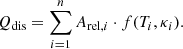
Test 3. Based on the measured charge-state distribution of iron ions of the same ICME as in Test 1 (No. 96 in our list), we generated 100 artificial ICME observations, each with its own charge-state distribution. The fraction of Fen+ is generated and re-normalized based on a normal distribution N(μ, σ2), where μ is the measured fraction of Fen+ in Case No. 96 and σ is the statistical uncertainty of this certain charge state. This means that the parameters of the populations of Case No. 96 are our target parameters, and we conduct this test to check the accuracy of our model for the identification of related parameters. All generated cases have been computed ten times with our model, which is sufficient according to Test. 1. Figure 2 reveals that our model is sensitive to the given charge-state distribution of iron ions. For cases with only minor differences, model results are different in the total number of majority populations in the first place. Among the 100 cases, 61 are identified as four-population, which is the same as in Case No. 96. However, the remaining 39 cases are three-population, and thus the total number of majority populations cannot be considered as a reliable criterion to distinguish ICME. For the 61 four-population cases, the modeled freeze-in temperatures and relative abundances of the four majority populations are (shown in mean-value±standard-deviation): MP1(6.00±0.09, 0.20±0.07), MP2(6.21±0.06, 0.30±0.05), MP3(6.41±0.05, 0.31±0.05), and MP4(6.97±0.1, 0.19±0.03). Compared to parameters of Case No. 96 shown in Fig. 1c, we can see our model is very good at identifying freeze-in temperature and shows less accuracy in determining relative abundance. As for the modeled κ on the other hand, we consider κ > 10 to be a large kappa value, indicating an approximate-Maxwellian distribution, and κ < 10 as a small kappa value. In that case, 57% of MP1 have a small κ of around 2.76±1.57; 59% of MP2 have a big κ, which is also the only population with a big κ in Case No. 96; 69% of MP3 have a small κ around 5.01±1.91; and 95% of MP4 have a small κ around 3.51±0.88. The hotter the population is, the more accurate our model is towards its κ. The modeled small κ is very close to the target value. The standard deviations for each parameter shown here are taken as a baseline estimate for the errors that come from a combination of the optimization, the statistical uncertainty of ACE, and the model itself. We carried out the same test on another case (No. 179 in our list) and use the same method to obtain the errors. The estimated errors are plotted in the following figures as a reference.
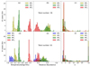 |
Fig. 2. Histograms of the parameters of the identified majority populations in 100 artificial ICME observations from Test. 3. The lines are provided by a KDE. Panels a–c are the results for 39 three-population cases and (d)–(f) show the results for 61 four-population cases. |
The 39 three-population cases also have two majority populations (MP2 and MP3 in Fig. 2a) with temperatures similar to MP3 and MP4 in Fig. 2d, and the parameters for the hot population are still close to the target values. However, most of the populations there have a small kappa and we cannot directly compare the results for the 39 three-population cases to those for our target case. The main difference between the three-population results and the four-population results is the absence of the coolest population around 1 MK. The temperature of the coolest population here (MP1) is above 1Mk and close to the temperature of MP2 in the four-population results.
This test demonstrates that our model is sensitive to the measurement uncertainty, and cases with three or four majority populations could be similar to each other. However, the identification of hot populations is clearly an advantage of our model, and the presence of hot populations can be considered as a reliable criterion for classification of ICMEs.
According to the above three tests, under the premise of multiple runs (ten for this work), our model is reliable, especially in identifying hot populations. Meanwhile, we have good reasons to accept the over fitting. Model results for freeze-in temperature are more reliable than the results for relative abundance and κ.
3. Model results for majority populations
In this section, we first describe our classification criteria together with several types of ICMEs based on this criteria. In Sect. 3.2, we then present our findings for the freeze-in temperature and the relative abundances of the different populations. The analysis of κ is presented in Sect. 3.3, and results related to other ICME properties are shown in the last subsection.
3.1. Classification criteria
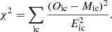
The criteria we use to classify ICMEs are based on the properties of the majority populations we find for each case. First, we divided all majority populations into two groups according to the freeze-in temperature with a threshold of 4 MK, one for cool populations and the other group for hot populations. This temperature threshold is selected based on a histogram of the temperatures of all the majority populations. There, the temperature threshold separates the hottest group of populations from the others. This threshold is shown as a black dashed line in Fig. 3. By doing this, all cases are classified as two main types, cool type and hot type, respectively lacking or possessing hot populations. Now, we label all ICME cases by the number of hot and cool populations our model identified in their iron charge-state distributions. This leads to eight sub-types of ICMEs, as listed in Table 1. However, only four of these types occur sufficiently frequently in our ICME data set, and so two subtypes of each main type (cool type and hot type) are included in the following analysis (Type B, Type C, Type F, and Type G).
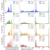 |
Fig. 3. Histogram of the parameters of the majority populations. From top to bottom are subplots for Type Cβ, Type Cα, Type Hβ, and Type Hα. From left to right are histograms for temperature, relative abundance, and κ of the majority populations that come from corresponding types with 50 bins, and bin ranges of [5.65, 7.2], [0.1, 0.9], and [1.55, 33], respectively. Different colors represent different populations in each type and populations are named independently; e.g., Cβ-pc1 represents cool population number one in Cβ, and Hβ-ph represents hot population in Type Hβ. The black dash line marks the temperature threshold to distinguish cool and hot populations, which is 4 MK. |
Number of cool majority populations and hot majority populations for each type and the total number of cases in each type.
In terms of number of cases, Type C is the most common type, with three cool populations and no hot populations. There are 145 Type C cases, almost half of the total. Type B is the second most frequent type, in which only two populations are needed to describe the charge-state distribution. There are 84 events identified with at least one hot majority population (hot type), which make up approximately 27% of the total. Among those “hot” types, Type G has the largest number of cases, with 53, followed by Type F with 24 cases. The numbers of cases for all other types are less than 2% of the total.
To facilitate further analysis, we renamed Type B, Type C, Type F, and Type G as Type Cβ, Type Cα, Type Hβ, and Type Hα, respectively. Here, “C” signifies a cool type of ICME with no hot majority populations, while “H” represents the hot type. α is used to signify the most frequent subtype, and therefore Cα means the most common cool type. The populations are then named according to their temperatures; for example, Cα-pc1 means the first cool population of type Cα in ascending order of temperature, Hα-ph means the hot population of type Hα.
3.2. Temperature and relative abundance
Four types of ICME are selected for further study (Type Cβ, Type Cα, Type Hβ, Type Hα). The histograms of parameters assigned to identify majority populations in those ICMEs are shown in Fig. 3.
For all types, the freeze-in temperatures of the majority populations are distinct. The temperatures of the two cool populations in Type Cβ are around 1.2 MK and 2 MK, respectively. For most cases of this type, Cβ-pc1 (∼1.2 MK) is more abundant, around 78%, but there are some events with a ratio (Cβ-pc1/Cβ-pc2) of 1:1. As another type that also does not contain any hot populations, Type Cα has three cool populations with temperatures of around 1 MK, 1.4 MK, and 2.4 MK. The relative abundance of Cα-pc1 is not as high as for Cβ-pc1. In terms of mean values of freeze-in temperature, Cα-pc1 is cooler than Cβ-pc1 while Cα-pc3 is hotter than Cβ-pc2. There are 24 cases that belong to Type Hβ, with two cool populations and one hot population (Hβ-ph, ∼7.9 MK). Hα-ph (∼6.6 MK) is slightly cooler than Hβ-ph and the other three cool populations are similar to those three in Type Cα with regard to temperatures. The fraction of hot populations (Hβ-ph and Hα-ph) is usually less than one-quarter in most respective ICME cases.
The freeze-in temperatures of cool populations in all four types follow the same trend, namely the distributions are more concentrated if a population has a higher temperature. We can see the peaks of Cβ-pc2, Cα-pc3, Hβ-pc2, and Hα-pc3 are the highest in the corresponding subplots. However, the temperatures of the hot populations exhibit the greatest variability. The relative abundance reveals very limited information because it could be strongly affected by the boundaries of ICMEs. The histograms of κ all have two peaks, one at the small value range from 1 to 5 and the other one at the maximum value; we analyze this κ value distribution in Sect. 3.3. We further compared the similarities and differences in freeze-in temperatures between several different populations of the four studied types and calculated the Pearson correlation coefficient and the Spearman rank correlaton coefficient (CCpearson and CCspearman), which have been marked on each subplot.
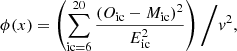
Both Type Cβ and Type Hβ have only two cool populations, namely Cβ-pc1 and Cβ-pc2, and Hβ-pc1 and Hα-pc2, respectively. Their freeze-in temperatures are plotted in Fig. 4a. Data points for Type Cβ (blue dots in Fig. 4a) have a broader distribution covering the range of data points for Type Hβ (orange crosses), which means the cool components of Type Cβ and Type Hβ could be similar, though the averaged temperature of Hβ-pc2 is higher than that of Cβ-pc2. As the histograms of freeze-in temperatures of Cβ-pc1 and Cβ-pc2 are similar to that of Cα-pc1 and Cα-pc3, we added data points for Type Cα (green triangles) together with data points for Type Hα (red pentagrams). Overall, the two distributions for the two cool subtypes are similar, with more than half of the overlapping areas visible in the figure. Though the most intuitive differences between Type Cα and Type Cβ are the number of cool populations or the occurrence of Cα-pc2, there is no significant difference between Type Cα and Type Cβ in terms of the freeze-in temperatures of the cool populations (same for Type Hα and Type Hβ). In all four types, pc1 has similar temperature ranges. We believe that the coolest population is related to solar wind-like material that is mixed into the ICME plasma.
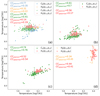 |
Fig. 4. Scatter plot for freeze-in temperatures of two selected populations in four types, details have been marked in the legend. Cβ(pc1,pc2) means the horizontal coordinate is the temperature of Cβ-pc1, while the vertical coordinate is the temperature of Cβ-pc2. The error bar for Case No. 96 estimated from Test. 3 is marked as well, together with the error bar for Case No. 179. (a) Scatter plot for freeze-in temperatures of Type Cα and Type Hα. (b) Scatter plot for freeze-in temperatures of two neighboring populations of Type Cα and Type Hα. (c) Scatter plot for freeze-in temperatures of two neighboring populations of Type Cα and Type Hα. (d) Scatter plot for freeze-in temperatures of hot populations and their neighboring populations of Type Hα and Type Hβ. |
The freeze-in temperatures of the other two pairs of neighboring populations of Cα and Type Hα were also compared in Fig. 4b,c, as well as hot populations and their neighboring populations of Type Hα and Type Hβ in Figs. 4d. In Figs. 4b,c, data points for Type Cα (green triangles) almost cover all the data points for Type Hα (red pentagrams), indicating that the cool parts of Type Cα and Type Hα have a very similar composition. Hot populations of the two hot subtypes also share a very similar distribution in Fig. 4d, which means Type Hα and Type Hβ are also similar in both cool and hot populations. Considering results from Test 3, there is no evidence that Type Hα and Type Hβ are two distinct subtypes of ICMEs with hot populations. The estimated errors shown here further demonstrate the similarity between the cool components of hot and cool types.
Furthermore, we find very good correlations for the green triangles in Fig. 4c, with a Pearson correlation coefficient as high as 0.74. A smaller correlation coefficient, but still above 0.6, was found in Fig. 4b, with a specific value at 0.61. Those two good correlations show that the freeze-in temperature of Cα-pc2 is related to the freeze-in temperature of Cα-pc1 and Cα-pc3. Meanwhile, the green triangles in Fig. 4a did not show a good correlation, indicating that the freeze-in temperatures of Cα-pc1 and Cα-pc3 are comparatively independent. The correlations between the neighboring cool populations are weaker in Type Hα than in Type Cα.
3.3. The κ value
Non-Maxwellian κ distributions have been widely detected in solar flares, active regions, the transition region, and the solar wind, which are potential source regions of plasma that our model identified in ICMEs. Our model did find a lot of populations of iron ions in ICMEs with a small κ below 5 (see Figs. 3c,f,i,l), but the number of populations with κ greater than 10 is also substantial.
According to the CHIANTI-kappa database, the charge-state distribution of iron ions in ionization equilibrium at the target temperature range of this work is actually stable and close to a Maxwellian distribution if κ is greater than 10, which is why we consider a κ of greater than 10 to signify an approximately Maxwellian distribution.
The charge-state distribution of iron ions is sensitive to κ of less than 5, representing an electron distribution that deviates significantly from a Maxwellian distribution. Table 2 shows the fractions of populations with κ in different value ranges. We can see that for cool subtypes, both big κ and small κ occupy more than 40%. The fraction of populations with a small κ is larger in hot subtypes, while the fraction of the population with medium κ is around 11% in all subtypes. We performed a further analysis of small κ for each majority population of the four studied subtypes of ICMEs mentioned above.
Fraction of populations with κ in different value ranges, respectively small, medium, and large.
Clearly, populations with a κ of below 5 are not uniformly distributed in a certain value range. In Fig. 5, we find several areas in which data points tend to be clustered, especially for pc1 (blue data points) in each subplot, which represents the coolest population in each ICME subtype.
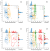 |
Fig. 5. Distribution of temperature and κ for each majority population of a certain type of ICME. A KDE plot is also provided in each subplot together with related histograms. For the histograms, there are 40 bins. κ here has been filtered to be no more than 5. The proportion of each data set that meets this criteria is as follows: (a) Type Cβ (66.7% C1, 28.2% C2). (b) Type Cα (77.9% C1, 22.1% C2, 21.4% C3). (c) Type Hβ (70.8% C1, 41.7% C2, 66.7% H). (d) Type Hα (83.0% C1, 26.4% C2, 24.5% C3, 86.8% H). |
According to Fig. 5a, for Type Cβ, which has 78×2 majority populations in total, 66.7% of pc1 are shown here and most of the κ values seen in pc1 are around 3.25 (see blue points in Fig. 5a). A few pc1 also have a smaller κ of around 2.0. κ for pc2 in this type tends to avoid the main area where blue data points are clustered, but with a smaller total number of data points (only 28.2%, see orange points in Fig. 5a).
There is also notable aggregation of data points for Type Cα in Fig. 5b. Here, the displayed κ values represent 77.9% of pc1. These κ values are gathered in two regions, the dominate one being around 2.25 with most of the cases, and the other being around 4.25, with fewer cases. The distribution of pc1 is different from that in Fig. 5a. Only 22.1% of pc2 (orange data points) and 21.4% of pc3 (green data points) have a κ of less than 5. pc2 shows a similar distribution to pc1, while pc3 is distributed similarly in the value range of [3, 5].
The total number of Type Hβ is only 24 but we can still find pc1 gathers around 3.25 (see blue points in Fig. 5c), similar to Cβ-pc1. Two-thirds of ph have a small κ but the distribution has a weak aggregation around 3.5.
Type Hα also shows a strong aggregation (see Fig. 5d). Distributions for pc1 and pc2 are different from Type Hβ but are similar to Type Cα, including pc3. The fraction of hot populations with small κ here is the biggest among all subtypes, up to 86.8%, and data points for ph are gathering in around 3.5. Combining Fig. 5b with Fig. 5d, as the two representative subtypes of cool- and hot-type ICMEs, Cα and Hα show strong similarity in the distribution of κ of the cool populations, including the related fractions of κ with a small value, and the difference is greater in the existence of hot populations.
According to the errors of Cases No. 96 and No. 178 estimated from Test 3 (see error bars in Figs. 5b,d), we believe that the existence of two cluster-in areas for κ of one single population (such as Cα-pc1 and Cα-pc2) does not necessarily imply that this population has two different source regions but may be a result of the uncertainty of our model.
3.4. Other properties of ICMEs
As shown in Fig. 6a, hot types (Type Hα and Type Hβ) were not identified during the solar-activity minimum, while they stand for 25% of all studied ICMEs during the solar-activity maximum and the fractions of Type Cβ and Type Hβ are both low during that time period. Hot populations are identified more frequently during years of solar-activity maximum, indicating that the source of that hot plasma is closely related to solar activity.
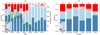 |
Fig. 6. Bar plots for the number of different types in terms of time, magnetic field structure and duration. (a) Yearly fractions of the four studied types of ICME, together with monthly sunspot number (Source: World Data Center, Sunspot Index and Long-term Solar Observations, Royal Observatory of Belgium, Brussels). Other types of ICMEs (10 cases in total) have been removed here and the number of cases in different groups is marked in the top of each bar. (b) Fraction of the four studied types of ICME in different groups (MC stands for magnetic cloud and the data shown are from R&C list. |
In the left panel of Fig. 6b, the fraction of Type Hα in magnetic clouds is clearly larger than that in not magnetic clouds, while the fraction of Type Hβ remains almost the same. In the right panel, we show the duration of each detected ICME based on the start time and end time from the R&C list and divided these into three groups, short-duration cases (< 18 h), medium-duration cases (18–36 h), and long-duration cases (> 36 h). From short-duration cases to long-duration cases, the fractions of Type Hα and Type Cα are both increasing. The duration of an ICME as detected by ACE is not one of the essential properties of ICMEs; and indeed this parameter could be effected by the relative motion velocity, the path of the spacecraft through the case, and the sizes and boundaries of the ICMEs themselves. But the longer the spacecraft stays inside the ICME and the more ICME material it detects, the more likely it is that our model is going to identify three cool populations, which lead to Type Hα and Type Cα. Since cases that are not magnetic clouds and have a short duration are less likely to be fully detected, Type Cβ could contain cases that are incomplete observations.
4. Discussion
We first discuss the limitations of our approach. Using the averaged charge-state distribution to represent the whole ICME period, which normally lasts dozens of hours, limits the interpretability of the model results by obscuring the temporal structure of the ICME. We cannot tell the temporal relationship between different populations of iron ions, and can therefore only generalize that all the populations are mixed. The averaged charge-state distribution is also affected strongly by the path of ACE through an ICME, as well as the boundaries of an ICME. While determining the boundaries between an ICME and the background solar wind is often highly subjective, it depends on which physical features the researchers choose to make the judgment, and so the identification of ICMEs in solar wind plasma and magnetic field data is still “something of an imprecise art” (Gosling 1990). Instead of compiling our own ICME list, we directly use the R&C list, which did not take iron charge distribution as its main criteria of ICME identification.
Not only can we not decipher whether the different identified populations are interrelated (and thereby observed at the same time) or are the result of the temporal or spatial structure of the ICME, but also we know that the specific path ACE takes through an ICME affects our results. Whether an ICME is detected completely be ACE is unknown to us, and an ICME period can also contain solar wind stream interaction regions or even another ICME. We cannot be sure that an ICME is not carrying hot material, nor that ACE simply did not pass through the hot material. Furthermore, if hot material only exists in a limited part of the ICME, then even if ACE goes through that hot material, its effect on the charge-state distribution is substantially reduced after averaging, which means that our model will not identify any hot populations, or at least not as a majority population, and the relative abundance of this population will be underestimated.
Another limitation of our approach is that we do not know whether the assumption that the respective coronal plasma is in ionization equilibrium is justified. This is another reason why the number of majority populations is less reliable; however, we still use that number to distinguish subtypes within two main types (hot type and cool type).
The four studied types of ICMEs identified in this work most likely do not correspond to four distinct kinds of eruption models. Relative abundances of different populations provide very limited direct information compared to the freeze-in temperature and κ.
The averaged charge-state distribution covers up a lot of details inside a single event, but can still be useful if we do a statistical study and look into the overall characteristics of this special type of solar wind. The different populations defined in the four studied types of ICMEs have their own features. These features suggest that they may originate from different source regions. Under the limitation that those features do not necessarily exist, they could be artificial or could be generated during the ejection or even during transport.
Coronal mass ejections are believed to be multicomponent and multitemperature and magnetic flux ropes are one of their important structural components. Cheng et al. (2011) divided the plasma of a CME could into three specific regions in temperature: the cool leading edge (compression front), the hot flux rope, and the mixed-temperature post-flare loops. The temperature of the hot flux rope could be as high as 10 MK according to observations from the Atmospheric Imaging Assembly (AIA) on board SDO (Cheng et al. 2011; Zhang et al. 2012). And the temperature of the cool leading edge is between 0.05 and 2.5 MK, which is estimated based on the observation by AIA at 211, 193, 171, and 304 Å in the same CME (Cheng et al. 2011). CMEs are also highly related to active regions. The temperatures of active-region structures range from 3 MK to 10 MK (Yoshida & Tsuneta 1996). In a recent work, measurements from the EUV imaging spectrometer (EIS), the X-ray Telescope (XRT) on Hinode, and AIA show that the differential emission measure in the active region core loops is sharply peaked at about 4 MK (Warren et al. 2020). Ishikawa & Krucker (2019), who studied hot plasma in a quiescent solar active region measured using the Ramaty High Energy Solar Spectroscopic Imager (RHESSI), XRT, and AIA, reported temperatures of up to 7 MK for active regions.
According to the results from the previous section, all ICMEs can be distinguished by the existence of hot majority populations into two main types, and these two types can then be divided into several subtypes. Among them, Cα is the most representative subtype of the cool type and Hα is the most representative subtype of the hot type.
In this study Cα is the most frequent cool type. This implies that it also could be a typical type of ICME. We interpret Cα-pc1 as typical coronal material. Cα-pc3 may come from active regions and is frequently associated with a Maxwellian electron distribution, that is, with large κ. The very weak correlation between the freeze-in temperature of Cα-pc1 and Cα-pc3 indicates that the source regions of Cα-pc1 and Cα-pc3 are relatively independent. This supports our interpretation that Cα-pc1 is solar-wind-like material. According to the good correlation found in Fig. 4c, one possibility is that pc2 could be a combination of two main parts, one coming from the heated Cα-pc1 and the other from the cooled Cα-pc3. The cooling process during the expansion could play a more important role in the formation of Cα-pc2 because the low frequency of the occurrence of small κ is similar to Cα-pc3. However, this could also be a model artifact: the model tries to compromise between different populations and attributes a (missed) minor population to the two detected populations.
It is worth noting that the averaged freeze-in temperature of Cβ-pc1 is between those of Cα-pc1 and Cα-pc2, while the mean freeze-in temperature of Cβ-pc2 is between those of Cα-pc2 and Cα-pc3. The role played by Cα-pc2 could be hidden in this temperature difference; otherwise Cβ-pc1 should be more similar to Cα-pc1. As Cβ is more often seen during the solar-activity minimum and in short-duration cases, it may be related to incomplete detection of ICMEs. The main difference between Cα and Cβ, which is the number of cool populations, is therefore more likely caused by the limitations of our model, which is based on single point observations. If the structure of an ICME is similar to that described by Cheng et al. (2011) or Song et al. (2016), and the outer layer of an ICME is therefore more frequently detected by spacecrafts, then plasma there could very likely be a cool type.
Type Hα is very likely another typical type of ICME and also a representative of the completely detected ICMEs, for they are more often seen in magnetic clouds and long-duration cases. In this type, Hα-pc1 is also around 1 MK and usually shows a small κ. pc2 is around 1.5 MK and Hα-pc3 could be from active regions with temperature ranges from 2 MK to 3 MK. We believe Hα-ph can be identified as the hot plasma around flux rope, normally showing a non-Maxwellian electron distribution, and Hβ-ph has a similar bias on κ. Furthermore, the cool part of Type Hα appears almost the same as Type Cα in freeze-in temperature and κ, and so the hot population could be more core-like in an ICME and our spacecraft would sometimes miss the detection of that hot core, which could lead to a Type Cα identification. Clearly, this type of ICME is suitable for further analysis of the heavy ion composition of each individual part in those cases. As in the case where Cβ is an incompletely detected subtype of the cool type, Type Hβ seems to be the defective subtype of the hot type, and therefore we consider Cα and Hα to be two representative subtypes.
pc1 in Cα, Cβ, and Hα are all solar-wind-like according to their temperatures, and are highly related to a non-Maxwellian electron distribution. The freeze-in temperature of Hβ-pc1 deviates from typical coronal material temperature. As the probability that ACE did not detect the ordinary coronal material during one single ICME period is low, but depending on the selection criteria, the respective part of the ICME might not be included in the start and end times from the R&C list, the boundaries of Type Hβ cases are worthy of further study.
The κ is a more interesting factor. The different determined κ values require a more nuanced interpretation. According to this work, non-Maxwellian electron distributions do exist widely in ICME material source regions, but it cannot be ignored that there is a considerable fraction of Maxwellian distributions, especially in mid-temperature populations (Cα-pc2, Cα-pc3, Hα-pc2, Hα-pc3). The fact that some of the populations appear to be in thermal equilibrium could suggest that they arise from longer-living, more stable structures in the corona and maintain this equilibrium during the ICME ejection mechanisms. According to the temperatures, those structures could be highly related to active regions. 1 MK material (pc1 in all types) usually has a small κ, and reference value ranges are [2.0, 2.5], [3.0, 3.5], and [4.0, 4.5]. The temperatures and κ of this population of plasma are similar to that of the solar wind detected by Ulysses (Maksimovic et al. 1997; Štverák et al. 2009). We find similar behavior for the hot populations (Hβ-ph, Hα-ph) with κ in the range of 3.0–4.5. Such hot plasma is rare among space plasma, and we notice the plasma sheet has an electron temperature of around 6.8±0.8 with a κ of around 4.0±1.0 (Kletzing et al. 2003); both parameters are similar in value to those of the hot populations identified by our model.
Gu et al. (2020) found that the averaged charge states of iron ions are highly related to the solar cycle. In the present work, those ICMEs with hot populations are also concentrated around the solar-activity maximum. However, the occurrence of those hot populations (Hβ-ph and Hα-ph) is not that closely related to the solar activity cycle compared to the averaged charge states of iron ions. When a high average charge state of iron is detected, it can sometimes be the result of the occurrence of populations with a very small κ. In other words, a high average charge state of iron does not necessarily imply the presence of a population with a higher freeze-in temperature. Also, the overall number of ICMEs during the solar-activity minimum phase is so low that we cannot rule out the possibility that we simply missed hot-type cases in our observations by chance.
5. Conclusions
In this work, we developed a multipopulation model based on a state-of-the-art optimization method, the CMA-ES, to describe the charge-state distributions of iron ions in ICMEs in detail. We analyzed averaged charge-state distributions of iron ions of 310 ICMEs from 1998 to 2011. We classify two main types of ICMEs according to the model results, namely cool type and hot type, and each has two relevant subtypes. Among the four studied subtypes of ICMEs detected at 1 AU by ACE, Type Cα and Type Hα are the most commonly seen types of ICMEs and Type Hα is most likely fully detected. Hα no doubt deserves further study because of the occurrence of the hot majority population. The occurrence of Hα is related to the solar cycle, and so the magnetic reconnection heating mechanism plays an important role.
The electron velocity distribution function usually contains a significant hot tail (indicating a kappa distribution) in typical coronal material and hot plasma, while the Maxwellian electron velocity distribution appears more frequently in mid-temperature material, and is possibly related to active regions.
Our multipopulation model can automatically diagnose any given charge-state distributions of iron ions, which makes our model suitable for other types of solar wind. The identified freeze-in temperatures and kappa index provide valuable information about the potential source regions of CME plasma.
The collaboration between the near-Sun remote sensing and the in situ measurement at different solar distances from Solar Orbiter (Müller 2020; Owen et al. 2020) and Parker Solar Probe (Bale et al. 2019) is expected to reveal details of the evolution of source components of ICMEs with the fine magnetic field structure, spectral temperature, and related distributions of charge states in situ.
http://www.srl.caltech.edu/ACE/ASC/level2/index.html (Retrieved September, 13, 2021).
http://www.srl.caltech.edu/ACE/ASC/DATA/level3/index.html (Retrieved April, 21, 2022).
Acknowledgments
This work is supported by China Scholarship Council (CSC) under the file number: 202106400008. S. Yao is supported by the National Natural Science Foundation of China under contract No. 42074204.
References
- Bale, S. D., Badman, S. T., Bonnell, J. W., et al. 2019, Nature, 576, 237 [NASA ADS] [CrossRef] [Google Scholar]
- Bame, S. J., Asbridge, J. R., Feldman, W. C., Fenimore, E. E., & Gosling, J. T. 1979, Sol. Phys., 62, 179 [NASA ADS] [CrossRef] [Google Scholar]
- Bochsler, P., Geiss, J., & Kunz, S. 1986, Sol. Phys., 103, 177 [NASA ADS] [CrossRef] [Google Scholar]
- Cane, H. V., & Richardson, I. G. 2003, J. Geophys. Res. (Space Phys.), 108, 1156 [NASA ADS] [CrossRef] [Google Scholar]
- Cheng, X., Zhang, J., Liu, Y., & Ding, M. D. 2011, ApJ, 732, L25 [NASA ADS] [CrossRef] [Google Scholar]
- Del Zanna, G., Polito, V., Dudík, J., et al. 2022, ApJ, 930, 61 [NASA ADS] [CrossRef] [Google Scholar]
- Dere, K. P., Landi, E., Mason, H. E., Monsignori Fossi, B. C., & Young, P. R. 1997, A&AS, 125, 149 [NASA ADS] [CrossRef] [EDP Sciences] [Google Scholar]
- Dudík, J., Dzifčáková, E., Meyer-Vernet, N., et al. 2017, Sol. Phys., 292, 100 [CrossRef] [Google Scholar]
- Dzifčáková, E., Dudík, J., Kotrč, P., Fárník, F., & Zemanová, A. 2015, ApJS, 217, 14 [CrossRef] [Google Scholar]
- Dzifčáková, E., Dudík, J., Zemanová, A., Lörinčík, J., & Karlický, M. 2021, ApJS, 257, 62 [CrossRef] [Google Scholar]
- Feng, X., Yao, S., Li, D., Li, G., & Yan, X. 2018, ApJ, 868, 124 [NASA ADS] [CrossRef] [Google Scholar]
- Geiss, J., Gloeckler, G., von Steiger, R., et al. 1995, Science, 268, 1033 [Google Scholar]
- Gloeckler, G., Cain, J., Ipavich, F. M., et al. 1998, Space Sci. Rev., 86, 497 [NASA ADS] [CrossRef] [Google Scholar]
- Gosling, J. T. 1990, Washington DC Am. Geophys. Union Geophys. Monogr. Ser., 58, 343 [NASA ADS] [Google Scholar]
- Gosling, J. T., Hildner, E., MacQueen, R. M., et al. 1974, J. Geophys. Rev., 79, 4581 [NASA ADS] [CrossRef] [Google Scholar]
- Gruesbeck, J. R., Lepri, S. T., Zurbuchen, T. H., & Antiochos, S. K. 2011, ApJ, 730, 103 [NASA ADS] [CrossRef] [Google Scholar]
- Gu, C., Yao, S., & Dai, L. 2020, ApJ, 900, 123 [NASA ADS] [CrossRef] [Google Scholar]
- Hansen, N. 2016, ArXiv e-prints [arXiv:1604.00772] [Google Scholar]
- Henke, T., Woch, J., Schwenn, R., et al. 2001, J. Geophys. Res. (Space Phys.), 106, 10597 [NASA ADS] [CrossRef] [Google Scholar]
- Ishikawa, S.-N., & Krucker, S. 2019, ApJ, 876, 111 [NASA ADS] [CrossRef] [Google Scholar]
- Kletzing, C. A., Scudder, J. D., Dors, E. E., & Curto, C. 2003, J. Geophys. Res. (Space Phys.), 108, 1360 [NASA ADS] [CrossRef] [Google Scholar]
- Kocher, M., Lepri, S. T., Landi, E., Zhao, L., & Manchester, W. B., IV et al., 2017, ApJ, 834, 147 [NASA ADS] [CrossRef] [Google Scholar]
- Kocher, M., Landi, E., & Lepri, S. T. 2018, ApJ, 860, 51 [NASA ADS] [CrossRef] [Google Scholar]
- Landi, E., Alexander, R. L., Gruesbeck, J. R., et al. 2012, ApJ, 744, 100 [NASA ADS] [CrossRef] [Google Scholar]
- Lepri, S. T., & Zurbuchen, T. H. 2010, ApJ, 723, L22 [Google Scholar]
- Lepri, S. T., Laming, J. M., Rakowski, C. E., & von Steiger, R. 2012, ApJ, 760, 105 [NASA ADS] [CrossRef] [Google Scholar]
- Lörinčík, J., Dudík, J., del Zanna, G., Dzifčáková, E., & Mason, H. E. 2020, ApJ, 893, 34 [CrossRef] [Google Scholar]
- Lynch, B. J., Reinard, A. A., Mulligan, T., et al. 2011, ApJ, 740, 112 [NASA ADS] [CrossRef] [Google Scholar]
- Maksimovic, M., Pierrard, V., & Riley, P. 1997, Geophys. Rev. Lett., 24, 1151 [NASA ADS] [CrossRef] [Google Scholar]
- Marsch, E. 2006, Liv. Rev. Sol. Phys., 3, 1 [Google Scholar]
- Müller, D., St Cyr, O. C., Zouganelis, I., et al. 2020, A&A, 642, A1 [Google Scholar]
- Nindos, A., Patsourakos, S., Vourlidas, A., & Tagikas, C. 2015, ApJ, 808, 117 [Google Scholar]
- Owen, C. J., Bruno, R., Livi, S., et al. 2020, A&A, 642, A16 [EDP Sciences] [Google Scholar]
- Richardson, I. G., & Cane, H. V. 2010, Sol. Phys., 264, 189 [NASA ADS] [CrossRef] [Google Scholar]
- Rivera, Y. J., Landi, E., Lepri, S. T., & Gilbert, J. A. 2019, ApJ, 874, 164 [NASA ADS] [CrossRef] [Google Scholar]
- Rodkin, D., Goryaev, F., Pagano, P., et al. 2017, Sol. Phys., 292, 90 [NASA ADS] [CrossRef] [Google Scholar]
- Song, H., & Yao, S. 2020, Sci. Chin. Technol. Sci., 63, 2171 [CrossRef] [Google Scholar]
- Song, H. Q., Zhong, Z., Chen, Y., et al. 2016, ApJS, 224, 27 [NASA ADS] [CrossRef] [Google Scholar]
- Song, H. Q., Chen, Y., Li, B., et al. 2017, ApJ, 836, L11 [NASA ADS] [CrossRef] [Google Scholar]
- Štverák, Š., Maksimovic, M., Trávníček, P. M., et al. 2009, J. Geophys. Res. (Space Phys.), 114, A05104 [NASA ADS] [Google Scholar]
- Tousey, R. 1973, Space Res. Conf., 2, 713 [Google Scholar]
- Warren, H. P., Reep, J. W., Crump, N. A., et al. 2020, ApJ, 896, 51 [NASA ADS] [CrossRef] [Google Scholar]
- Wimmer-Schweingruber, R. F. 2006, Space Sci. Rev., 123, 471 [NASA ADS] [CrossRef] [Google Scholar]
- Wimmer-Schweingruber, R. F., Crooker, N. U., Balogh, A., et al. 2006, Space Sci. Rev., 123, 177 [Google Scholar]
- Yoshida, T., & Tsuneta, S. 1996, ApJ, 459, 342 [NASA ADS] [CrossRef] [Google Scholar]
- Zhang, J., Cheng, X., & Ding, M.-D. 2012, Nat. Commun., 3, 747 [Google Scholar]
Appendix A: Model results
The entire table listing the model results of the 310 ICMEs studied here is available at the CDS.
All Tables
Number of cool majority populations and hot majority populations for each type and the total number of cases in each type.
Fraction of populations with κ in different value ranges, respectively small, medium, and large.
All Figures
|
Fig. 1. Measured and modeled charge-state distributions of iron ions of four selected ICMEs. The case numbers of the four ICMEs are marked in each subplot and detailed parameters of populations are given in the form of pn(T, Arel, κ). All distributions are normalized to their respective sum and the error bars indicate the observational uncertainty. |
| In the text | |
|
Fig. 2. Histograms of the parameters of the identified majority populations in 100 artificial ICME observations from Test. 3. The lines are provided by a KDE. Panels a–c are the results for 39 three-population cases and (d)–(f) show the results for 61 four-population cases. |
| In the text | |
|
Fig. 3. Histogram of the parameters of the majority populations. From top to bottom are subplots for Type Cβ, Type Cα, Type Hβ, and Type Hα. From left to right are histograms for temperature, relative abundance, and κ of the majority populations that come from corresponding types with 50 bins, and bin ranges of [5.65, 7.2], [0.1, 0.9], and [1.55, 33], respectively. Different colors represent different populations in each type and populations are named independently; e.g., Cβ-pc1 represents cool population number one in Cβ, and Hβ-ph represents hot population in Type Hβ. The black dash line marks the temperature threshold to distinguish cool and hot populations, which is 4 MK. |
| In the text | |
|
Fig. 4. Scatter plot for freeze-in temperatures of two selected populations in four types, details have been marked in the legend. Cβ(pc1,pc2) means the horizontal coordinate is the temperature of Cβ-pc1, while the vertical coordinate is the temperature of Cβ-pc2. The error bar for Case No. 96 estimated from Test. 3 is marked as well, together with the error bar for Case No. 179. (a) Scatter plot for freeze-in temperatures of Type Cα and Type Hα. (b) Scatter plot for freeze-in temperatures of two neighboring populations of Type Cα and Type Hα. (c) Scatter plot for freeze-in temperatures of two neighboring populations of Type Cα and Type Hα. (d) Scatter plot for freeze-in temperatures of hot populations and their neighboring populations of Type Hα and Type Hβ. |
| In the text | |
|
Fig. 5. Distribution of temperature and κ for each majority population of a certain type of ICME. A KDE plot is also provided in each subplot together with related histograms. For the histograms, there are 40 bins. κ here has been filtered to be no more than 5. The proportion of each data set that meets this criteria is as follows: (a) Type Cβ (66.7% C1, 28.2% C2). (b) Type Cα (77.9% C1, 22.1% C2, 21.4% C3). (c) Type Hβ (70.8% C1, 41.7% C2, 66.7% H). (d) Type Hα (83.0% C1, 26.4% C2, 24.5% C3, 86.8% H). |
| In the text | |
|
Fig. 6. Bar plots for the number of different types in terms of time, magnetic field structure and duration. (a) Yearly fractions of the four studied types of ICME, together with monthly sunspot number (Source: World Data Center, Sunspot Index and Long-term Solar Observations, Royal Observatory of Belgium, Brussels). Other types of ICMEs (10 cases in total) have been removed here and the number of cases in different groups is marked in the top of each bar. (b) Fraction of the four studied types of ICME in different groups (MC stands for magnetic cloud and the data shown are from R&C list. |
| In the text | |
Current usage metrics show cumulative count of Article Views (full-text article views including HTML views, PDF and ePub downloads, according to the available data) and Abstracts Views on Vision4Press platform.
Data correspond to usage on the plateform after 2015. The current usage metrics is available 48-96 hours after online publication and is updated daily on week days.
Initial download of the metrics may take a while.