| Issue |
A&A
Volume 687, July 2024
|
|
|---|---|---|
| Article Number | A75 | |
| Number of page(s) | 9 | |
| Section | Interstellar and circumstellar matter | |
| DOI | https://doi.org/10.1051/0004-6361/202245338 | |
| Published online | 01 July 2024 | |
Spatial distributions of PN and PO in the shock region L1157-B1
1
Univ. Grenoble Alpes, CNRS, IPAG,
38000
Grenoble,
France
e-mail: bertrand.le-floch@u-bordeaux.fr
2
Laboratoire d’astrophysique de Bordeaux, Univ. Bordeaux, CNRS, B18N, allée Geoffroy Saint-Hilaire,
33615
Pessac,
France
3
INAF, Osservatorio Astrofisico di Arcetri,
Largo E. Fermi 5,
50125
Firenze,
Italy
e-mail: claudio.codella@inaf.it
4
LESIA, Observatoire de Paris, Université PSL, CNRS, Sorbonne Université, Université Paris Cité,
5 place Jules Janssen,
92195
Meudon,
France
5
IRAP, Université de Toulouse,
9 avenue du colone Roche,
31028
Toulouse Cedex 4,
France
6
Leiden Observatory, Leiden University,
PO Box 9513,
2300 RA
Leiden,
The Netherlands
7
Department of Physics and Astronomy, UCL,
Gower St.,
London
WC1E 6BT,
UK
8
Centro de Astrobiologia (CSIC/INTA), Ctra de Torrejón a Ajalvir,
km 4 Torrejón de Ardoz,
28850
Madrid,
Spain
Received:
31
October
2022
Accepted:
2
April
2024
Phosphorus plays an essential role in prebiotic chemistry. The origin of P-bearing molecules in the protostellar gas remains highly uncertain. Only PO and PN have been detected towards low-mass star-forming regions and their emission is mainly associated with outflow shocks. In order to make progress in the characterisation of P-chemistry, we present NOEMA observations of PO and PN at 3″−4″ resolution towards the outflow shock region L1157-B1. Our resolved observations confirm the association of both P species with the apex of the bow shock. High-velocity emission is detected in the compact region where the jet impacts the shock. Analysis of the spatial distributions of PO and PN indicates that these molecules are not sputtered from the icy mantles of dust grains; they are the gas-phase products of a P-mother species released in the shock. PO appears to form first in the gas phase, followed by PN, which remains longer in the shock, when PO is no longer detected. Variations of the PO/PN abundance ratio in the range 1–5 are detected over the apex and confirm the short time variability of P-chemistry, which typically lasts a few hundred years. These results are consistent with the previous modelling of P-chemistry in L1157-B1. Complementary observations of N-bearing species at high angular resolution are needed to better understand the formation pathways of PO and PN.
Key words: astrochemistry / stars: formation / ISM: jets and outflows / ISM: molecules / ISM: individual objects: L1157
© The Authors 2024
 Open Access article, published by EDP Sciences, under the terms of the Creative Commons Attribution License (https://creativecommons.org/licenses/by/4.0), which permits unrestricted use, distribution, and reproduction in any medium, provided the original work is properly cited.
This article is published in open access under the Subscribe to Open model. Subscribe to A&A to support open access publication.
1 Introduction
Phosphorus plays a key role in prebiotic chemistry. As has been stressed by many authors (see e.g. Macia 2005), the PO bond plays an important role in the energy storage role in all living beings on Earth. It is also part of the backbone of ribonucleic acid (RNA) and deoxyribonucleic acid (DNA). Its recent signature detection in the material of comet 67P by Altwegg et al. (2016) stimulated several authors to study this element in order to better understand its evolutionary path in the chemical heritage of our Solar System from the early prestellar phase. So far, no evidence has been found of P-bearing species detected in protoplanetary discs, although in our Solar System, phosphine PH3 has been detected in the Jovian atmosphere (Ridgway 1974). Also, phosphorus-bearing compounds are detected in minerals of rocky planets with an abundance higher than its cosmic ranking and are ubiquitous in meteorites and in interplanetary dust particles (Macia 2005). The recent Rosetta mission detected the signature of ionised phosphorus in the coma of comet 67P (Altwegg et al. 2016) and after an in-depth analysis of the ROSINA data, Rivilla et al. (2020) concluded that PO is most likely the main carrier of P in the comet with a large relative abundance ratio of PO/PN > 10.
In the diffuse interstellar medium, phosphorus is detected mainly in the ionised form, P+ (Jura & York 1978), with low depletion factors – of the order of a few – with respect to the solar value of 3 × 10⁻⁷ (Anders & Grevesse 1989; Asplund et al. 2009). The situation is different in dense molecular clouds, where PN is detected with abundances in the range of 10−12−10−10 with respect to H2, which suggests that phosphorus is most likely depleted onto dust grains (Turner et al. 1990).
The species PO and PN have been detected in quite a large sample of high-mass star-forming regions at different evolutionary stages, from starless to protostellar cores and ultracompact HII regions (Fontani et al. 2016; Mininni et al. 2018; Fontani et al. 2019; Rivilla et al. 2020; Bernal 2021). In general, the PN and PO spectral line profiles are found to be well correlated with those of shock tracers such as SiO (Rivilla et al. 2018; Fontani et al. 2019). However, in a few objects, PN is found to arise from relatively quiescent gas, suggesting the possibility of different formation pathways for this species (Fontani et al. 2016).
On the other hand, P-bearing species PN and PO have only been detected in a few low-mass star-forming regions: protostellar shock L1157-B1 (Lefloch et al. 2016), Class 0 NGC1333-IRAS4A, the young protostellar core B1-b (Lefloch et al. 2018), and Class I B1a (Bergner et al. 2019, 2022) in the Perseus molecular cloud.
In the protostellar shock L1157-B1 (d=352 pc, Zucker et al. 2019), the similarity between the profiles of the PN and SiO rotational transitions J = 2–1 led Lefloch et al. (2016) to propose that the PN emission arises from the shocked gas too. Interestingly, the PO and PN rotational line profiles appear to display different spectroscopic signatures, suggesting their emission arises from spatially distinct regions. These observational results were supported by a detailed shock modelling of the PO and PN emission. However, the lack of angular resolution of the IRAM 30 m telescope (about 25″ in the 3mm window) with respect to the size of L1157-B1 (~10″) prevents any firm conclusions as to the spatial distribution and the origin of PO/PN in the shock. It is necessary to image the emission of PO and PN at high spatial resolution to address these questions.
Here, we present emission maps of PO and PN rotational transitions in the 3mm range towards L1157-B1 obtained with the NOEMA interferometer at 3″ resolution. Section 2 describes the observations. Our results on the distribution of PN and PO in the shock are described in Sect. 3. In Sec. 4, we then discuss the differences observed between PO and PN, and the implications for the origin of both species in relation to the time evolution of the outflow. Finally, our conclusions are presented in Sec. 5.
PN and PO lines observed with the IRAM NOEMA interferometer in the D configuration.
2 Observations
2.1 NOEMA observations
The L1157-B1 protostellar shock region was observed at 3 mm in February and March 2017 with NOEMA in its seven- and eight-antenna configurations (7D and 8D, respectively). The line PN N = 2–1 line (see Table 1) was observed on 8 February, 17 February, and 3 March 2017. The PO 2Π1/2 J = 5/2–3/2 lines (Table 1) were observed simultaneously on 10, 11, 14, and 17 February. Both instrumental settings were observed in D configuration in a single field centred at the nominal position of L1157-B1 α(2000) = 20h39m10s.2, δ(2000) = +68°01′10.5″. The antenna baselines sampled in our observations range from 15 m to 127 m, therefore allowing us to recover emission up to a maximum scale of 41″. The PN lines were observed in a spectral band of 160 MHz with a resolution of 625 kHz (≈2 km s−1). The PO transitions were observed in two spectral bands of 160 MHz bandwith and 625 kHz resolution. The instrumental setup is summarised in Table 1.
Calibration and data analysis were carried out following standard procedures with the GILDAS-CLIC-MAPPING software2. The RF bandpass was calibrated on 3C273 and 2200+420 (for PN observations) and 3C84 and 2013+370 (for PO observations). The absolute flux scale was determined from observations of MWC349 and LkHα101. The phase and amplitudes were calibrated using 2010+723 and 1928+738. The phase rms was ≤25°, pwv was 2–10 mm, and system temperatures were ~60–200 K, leading to less than 1% flagging in the dataset. Images were produced using a natural weighting and restored with a clean beam of 4.47″ × 3.58″ and PA = +88° for PN J = 2–1 and 3.46″ × 3.37″ and PA = +82° for PO J = 5/2–3/2. The final uncertainty on the absolute flux calibration is ≤10% at 3 mm. The intensity per spectral channel (625 kHz) can be converted from Jy beam−1 to brightness temperature units (TB) using the conversion factor TB(K) = 8.65 × F (Jy beam−1). The typical rms noise per spectral channel of 625 kHz is ~0.012 K and ~0.010 K in the PN and PO images, respectively (see Fig. 1).
2.2 Comparison of the IRAM 30 m and NOEMA data
Figure 2 shows a comparison of the distributions of the PN N = 2–1 flux density as observed with ASAI using the IRAM 30 m antenna (magenta, Lefloch et al. 2016) and the equivalent flux obtained from the NOEMA spectrum extracted from the map (black) in a circular region with a solid angle equal to the IRAM 30 m HPBW. The vertical dot-dashed line marks the systemic velocity of L1157-mm. The blue lines indicate the frequencies of the ΔJ =0, ±1 transitions of the N = 2–1 pattern. The length of the lines is proportional to the relative line strength (see Table 1). We conclude that most of the flux of the PN 2–1 line detected by the IRAM 30m is also recovered by NOEMA.
3 Results
We first assessed the spatial distribution of the PN and PO line emission obtained with NOEMA in the B1 region. We investigated the spatial distribution of the species in the shock and we discuss the constraints brought by these observations on the abundance of PO and PN in the shock region.
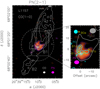 |
Fig. 1 Phosphorus-bearing molecules in the L1157-B1 protostellar shock. Left: emission map of the PN N = 2–1 line obtained with NOEMA in the southern lobe of the L1157 outflow. The emission (colour) is integrated in the velocity range −10 to +5 km s−1. The first contour and contour interval (blue) are 3σ (36 mJy beam−1 km s−1) and 2σ, respectively. The dashed white circle shows the primary beam of the PN image (53″). The CO J = 1–0 outflow emission, as imaged by Gueth et al. (1996) is superimposed in white contours. The white triangle at the top points to the position of the L1157-mm protostar. Right: magnified view of the L1157-B1 central region. The maps are centred at: α(J2000) = 20h39m 10s.2, δ(J2000) = +68°01′10.″5. The PN N = 2–1 map is compared with the stacked intensity distribution of PO J = 5/23/2, F = 3–2, ef (cyan thick contours). The first contour and contour interval of the PO map are 3σ (21 mJy beam−1 km s−1) and 2σ respectively. The 3σ level of the p-H2CO J = 20,2−10,1 integrated emission (Benedettini et al. 2013; grey contours) is here used to define the whole structure of the B1 shock. The cyan ellipse draws the synthesised beam of the PO observations, and shock knots B1a-B1b-B1c-B0e are marked by yellow triangles. |
3.1 PN
3.1.1 Spatial distribution
The spatial distribution of the PN N = 2–1 line flux – which is dominated by the J = 2–1 component – integrated in the velocity range [−11.3; +6.6]km s−1 is shown in colour scale in Fig. 1. A detailed view of the distribution of PN N = 2–1 emission as a function of velocity is displayed in Fig. 3. The emission map reveals two main components with different morphologies: (a) a low-velocity, extended component is detected mainly in the range [−5.5;+4.4] km s−1, and (b) a high-velocity, compact component detected in the range [−10;−5.5] km s−1.
As can be seen in Fig. 1, the PN emission appears to be mainly located at the apex of the B1 cavity, well traced by CO J = 1–0 (Gueth et al. 1996) and H2CO (Benedettini et al. 2013), where it delineates a region of about 15″ in diameter, which is therefore fully resolved by the 4.5″ × 3.6″ synthetic beam of the observations. There is no evidence of any other emission structure inside the primary beam of the instrument, in particular towards the shock position B0e at about 20″ northeast of B1c (Benedettini et al. 2007, 2013).
The PN brightness peak is located 4″ south of the B1 nominal position adopted, close to B1c. The corresponding PN line spectrum is displayed in the top panel of Fig. 4. With a brightness peak intensity of 17 mJy beam−1 (0.156 K), the line is detected at better than 12σ in our NOEMA observations and is approximately five times as bright as the line detected in the IRAM 30 m telescope beam.
We compared the PN N = 2–1 line observed in ASAI with the IRAM 30 m telescope (Lefloch et al. 2016) and the equivalent NOEMA spectrum. As can be seen in the top panel of Fig. 2, a very good match is observed between the two spectra. In particular, the emission peaks at velocities close to −0.5 km s−1, slightly blueshifted with respect to the ambient cloud velocity (Vlsr = +2.7 km s−1, Bachiller et al. 2001), and extends up to −15 km s−1. Overall, NOEMA recovered 85% of the PN N = 2–1 flux collected with the IRAM 30 m telescope. Therefore, PN arises from the apex of the outflow cavity and originates from the shock L1157-B1 itself.
As can be seen in the right panel of Fig. 5 (also Fig. 3), the low-velocity PN component in the velocity interval V = −4.5-+1.4 km s−1 traces the apex of the B1 outflow cavity, and reaches its maximum intensity at the location of B1c. There is no evidence of a velocity gradient in the low-velocity component across the emitting region. A comparison with the low-velocity emission of the SiO J = 2–1 line observed at 2.″8 × 2.″2 by Gueth et al. (1998) shows that the overall spatial distributions are similar (Fig. 5). This explains the very good match observed by Lefloch et al. (2016) between the spectroscopic signatures of the PN N = 2–1 and SiO J = 2–1 transitions at the angular resolution of the IRAM 30 m telescope (25″−28″).
However, two differences can be noted in the low-velocity emission: (a) on the eastern side, the PN emission appears slightly shifted to the south; and (b) the PN and SiO emission peaks coincide with knots B1c and B1a, respectively, which are ~8″ apart. Interestingly, our PN data reveal a counterpart to the ‘SiO finger’ ahead of the bow (−14″ < Δδ < −10″), which Gueth et al. (1998) interpreted as a trace of jet-shocked material.
As mentioned above, a secondary emission peak is detected in the high-velocity regime, at velocities between −5.3 and −13 km s−1, with respect to the ambient gas velocity, as can be seen in the channel maps of Fig. 3. This finding is noted also in Fig. 6, where the PN N = 2–1 line spectra observed towards the knots B1a and B1c are shown. At both positions, the spectra display clear evidence of the two components: a low-velocity component between −5.3 and +4.6 km s−1, and a high-velocity component between −14 and −5.3 km s−1.
On the other hand, the distribution of the high-velocity PN emission between −11 km s−1 and −5.3 km s−1 (see Figs. 3 and 5) draws a more contrasted picture, as the bulk of emission is limited to a compact, marginally resolved region of ≈4″ in diameter towards B1c, and towards B1a at a lower level. The emission peak coincides with the location of knot B1c. Whereas the PN emission peaks at V ≃ −6 km s−1 towards B1c (see Fig. 6), it appears to peak at higher velocities of close to −10 km s−1 towards B1a, where the protostellar jet impacts the cavity (Benedettini et al. 2012). The distribution of the highvelocity SiO emission compared with the structure of jet-driven bowshocks (Raga & Cabrit 1993) suggests that the emission arises from a different part of the shock, possibly the jet impact region, associated with more stringent shock conditions, possibly dissociative and/or J-type, based on the OI and high-J CO emission detected in the region with Herschel (Benedettini et al. 2012). This suggests that the high-velocity PN emission traces the jet interaction with the ambient material.
Our NOEMA observations provide very detailed information on the structure of the PN emission, and confirm the hypothesis proposed by Lefloch et al. (2016) that the PN emission arises from the region traced by SiO in the shock. NOEMA also allows us to exclude the possibility raised in this previous work that the bulk of PN emission would arise from small ‘knots’ such as B1a,b,c.
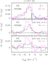 |
Fig. 2 Top: comparison in flux density scale between the PN and PO spectra as observed using the IRAM 30 m antenna (magenta, Lefloch et al. 2016) and that extracted from the NOEMA map (black) from a circular region equal to the IRAM 30m HPBW. Top: PN N= 2–1 spectra. The HPBW is 26″.2. The vertical dot-dashed line marks the systemic velocity of L1157-mm (V = +2.7 km s−1). The blue lines indicate the frequencies of the ΔJ = 0, ±1 transitions of the N = 2–1 pattern (see Table 1). Middle: same as in the top panel but for the PO 2Π1/2 J = 5/2–3/2 F = 3–2 f transition (IRAM 30 m beam: 22″.6). Bottom: same as in the middle panel but for the PO transition 2Π1/2 J = 5/2–3/2 F = 3–2 e. |
3.1.2 Molecular abundance
We used the MADEX radiative transfer code (Cernicharo 2012) to run a non-local thermodynamic equilibrium (NLTE) Large Velocity Gradient (LVG) analysis of the PN N = 2–1 line and determine the PN column density necessary to reproduce the intensities measured with NOEMA. We adopted the PN-He collisional coefficients of Tobola et al. (2007), scaled by a factor of 1.37 to take into account the difference in mass of H2. We adopted the temperature (70 K) and density (0.9 × 105 cm−3) as estimated by Lefloch et al. (2016) for the PN lines, in agreement with the fact that NOEMA recovered most of the flux (85%) of the IRAM 30m observations. These physical conditions are consistent with those estimated from a multi-transition analysis of CO and CS at the apex of the L1157 bow shock (Lefloch et al. 2012; Gómez-Ruiz et al. 2015). Also, we adopt line widths of ΔV = 6–8 km s−1, depending on the line profiles.
At the brightness peak we measure TB = 0.16 K (Fig. 4), and MADEX gives N(PN) ≃ 2.3 × 1012 cm−2. The PN transitions in the millimetre domain are predicted to have rather low excitation temperatures of ~10 K. Adopting the CO column density for the B1 cavity of 1 × 1017 cm−2 (Lefloch et al. 2012) and a standard abundance ratio [CO]/[H2] = 10−4, the abundance of PN relative to H2 is then 2.8 × 10⁻⁹. This value is about three times as high as the determination based on the IRAM 30m data (Lefloch et al. 2016). Interestingly, integrating the H2 density of the PN emitting region (0.9 × 105 cm−3) over a distance of 15″, corresponding to the PN size measured in the plane of the sky, one obtains a total column density N(H2) ≃ 7 × 1021 cm−2, which is about seven times higher than the value determined from CO (Lefloch et al. 2012). Both approaches can be easily reconciled if the PN-emitting region is not a sphere uniformly filled with PN but rather a layer of about 2″ thickness, still with the same H2 density, which would be coherent with the geometry of a jet-driven bow shock.
High-velocity PN emission is detected towards knots B1c and B1a (Figs. 5–6). Following the same procedure as above, we estimated the column density N(PN) at these positions under the assumption of similar physical conditions to those in the B1 cavity. The values are reported in Table 2. Complementary observations from higher-excitation PN lines and at high sensitivity and similar angular resolution would help to reduce the uncertainties on the physical conditions in B1a and B1c.
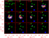 |
Fig. 3 Spatial distribution of the PN N = 2–1 emission as a function of velocity, as observed with NOEMA, between −14 km s−1 and +7.4 km s−1. Each velocity channel has a width of 2 km s−1. The velocity is marked in red in the top left corner of each panel. The synthesised beam is depicted by a blue ellipse in the bottom right corner. First contour and contour interval (in blue) are 3σ and 1σ of the flux distribution, respectively. The location of the shock knots B1a-B1c and B0e are marked by green crosses. |
3.2 PO
We detected emission from the PO transitions: 2Π1/2 J=5/2–3/2, F=3–2, e, and f (see Table 1). Figure 2 displays the comparison of PO spectra as extracted from the NOEMA images with those of IRAM 30 m ASAI: in this case, the interferometer recovered ~50–60% of the flux measured by the single-dish telescope in a beam of 26.2″. The low signal-to-noise ratio (S/N) of ~3–4 could affect the comparison, but it seems that a fraction of the flux is filtered out by the interferometer. This suggests that in addition to the structure reported in Fig. 1, PO is also associated with a molecular structure larger than the recovered scale (34″), which in turn implies that part of the PO emission is associated with the extended outflow cavities.
In order to gain insight into the PO distribution, we stacked both transitions and present the resulting map in the right panel of Fig. 1. As for PN, the PO emission imaged by NOEMA is confined close to the apex of the B1 outflow cavity. Interestingly, the PO emission appears slightly shifted towards the north with respect to PN. The region of highest PO brightness (Fig. 1) appears to coincide with the high-velocity jet emission region, as traced by SiO J=2–1 (left panel of Fig. 5).
Figure 4 (bottom panel) shows the spectrum obtained by stacking the 2Π1/2 J=5/2–3/2, F=3–2, e, and f lines extracted at the peak position of the PO map reported in Fig. 1: α(2000) = 20h39m10s.4, δ(2000) = +68°01′08.4″. The PO emission appears to peak at velocities close to −5 km s−1, blueshifted with respect to the average PN emission spectrum (Fig. 4), but in rather good agreement with the high-velocity PN component detected towards B1c (Fig. 6) in the jet emission region. We note that the PO emission is not bright enough to allow a detailed kinematical analysis.
In order to estimate the PO column density at the same positions as for PN in the shock, we adopted the same approach as Lefloch et al. (2016) and in the absence of coefficients available for H2-PO collisions, and we carried out an LTE analysis of the PO 2Π1/2 J=5/2–3/2 e 3–2 line using CASSIS3 (Vastel et al. 2015), adopting the excitation temperature (12 K) estimated by Lefloch et al. (2016) from a PO multi-line analysis with the IRAM 30 m telescope. The PO column density lies in the range 3.5–5.0 ×1012 cm−2. The results of our LTE analysis are summarised in Table 2 and provide information showing some trends in the variations of the PO/PN ratio across the shock region. The PO/PN ratio varies from ~1.5 to 4.7, in agreement with previous studies of interstellar regions (see e.g. Rivilla et al. 2016, 2018; Bergner et al. 2019). As expected, the lower values are observed towards the PN emission peak (LV and HV) and the higher values towards the PO emission peak. In the high-velocity gas possibly associated with the jet impact shock region, we measure a value of 4.7 towards B1a, whereas this value is about 1.5 lower towards B1c (2.9), a region older by about 140 yr, based on the modelling by Podio et al. (2016). The same trend is observed when considering the whole PO/PN line flux distribution as the ratio is found to increase by a factor of approximately 3. These findings need to be verified once the collisional coefficients of PO are available in order to make a comparison between PO and PN column densities both derived using the NLTE LVG approach.
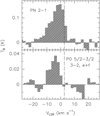 |
Fig. 4 PN and PO spectra. Top: PN N = 2–1 spectrum at the peak of the PN spatial distribution. The vertical dot-dashed line marks the systemic velocity of L1157-mm. Bottom: PO emission at the peak of the spatial distribution obtained by stacking the lines 2Π1/2 J = 5/2–3/2, F = 3–2 f and 2Π1/2 J = 5/2–3/2 F = 3–2 e. Intensities are expressed in TB scale. |
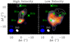 |
Fig. 5 Comparison of the PN N = 2–1 and SiO J = 2–1 line emissions. Left: high-velocity range. The PN N = 2–1 line flux (colourscale and red contours) is integrated in the velocity interval [−11;−5.3] km s−1; the first contour and contour interval are 3σ (1.8 × 10⁻² Jy beam−1 km s−1) and 2σ (1.2 × 10⁻² Jy beam−1 km s−1), respectively. The SiO J = 2–1 emission (white contours) is integrated in the velocity interval [−19.7;−6.7] km s−1; the first contour and contour interval are 20% and 15% of the SiO peak intensity, respectively. Right: low-velocity range. The PN N = 2–1 line flux is integrated in the velocity interval [−5.3;+4.6] km s−1; the first contour and contour interval are 3σ (2.5 × 10⁻² Jy beam−1 km s−1) and 2σ (1.6 × 10⁻² Jy beam−1 km s−1), respectively. The SiO J = 2–1 emission is integrated in the velocity interval [−6.7; +3.7] km s−1; the first contour and contour interval are 20% and 15% of the SiO peak intensity, respectively. The red and white ellipses depict the synthesised beams of the PN N = 2–1 and SiO J = 2–1 observations, respectively. Coordinates are in arcsecond offsets with respect to the nominal position of B1. |
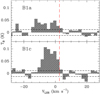 |
Fig. 6 PN N = 2–1 emission detected with NOEMA towards shock positions B1a (top) and B1c (bottom). Line intensities are expressed in TB scale. The vertical red dashed line marks the systemic velocity of L1157-mm. The horizontal black dashed line marks the 1σ noise level of the spectrum (12 mK). |
Column densities of PN and PO determined at the shock positions B1a and B1c and at the emission peaks of the PN N = 2–1 and PO 2Π1/2 J = 5/2–3/2 e 3–2 (108998 MHz) lines.
4 Discussion
4.1 Origin of the P-molecules in the shock
The chemical structure of L1157-B1 and the above results are tightly connected with the physical structure of the outflow, which displays evidence of time variability and precession (Gueth et al. 1996). The shock regions B0-B1-B2 trace the impact of the L1157 protostellar jet against the outflow cavity. As a consequence of the change of jet propagation direction induced by precession, the location of its impact against the outflow cavity appears to move in the northern direction, from B2 to B0. In their study of NH2CHO in L1157-B1, Codella et al. (2017) concluded that this gradient is present inside the bow shock. The L1157 outflow precession was modelled in a detailed manner by Podio et al. (2016), and adopting the new Gaia distance of 350 pc, accurate age estimates of 1540 yr and 1680 yr were obtained for knots B1a and B1c, respectively.
As seen in the previous section, very good agreement is observed between the spatial distributions of PN and SiO. It is well established that the bulk of silicon (about 90%) is stored in the cores of the interstellar grains under the form of silicates, such as olivine, forsterite, and fayalite (see e.g. May et al. 2000). Sputtering of dust grain cores in high-velocity shocks (≥20–25 km s−1) leads to the release of silicon in the gas phase. Silicon subsequently reacts with O2 or OH to produce SiO (Gusdorf et al. 2008; Codella et al. 2017).
Some shock codes (like e.g. Paris-Durham, Flower & Pineau des Forets 2003) consider that a fraction of silicon (5–10%) stored at the surface layers of dust grains is sufficient to successfully reproduce the observations of shocks in some low-and high-mass star forming regions (Gusdorf et al. 2008, 2015; Leurini et al. 2014). The good match observed between the PN and the SiO spatial distributions in the low-velocity component (Fig. 5) strongly suggests that PN arises from shocked material and actually forms in the gas phase.
This result is consistent with the lack of correlation found between the spatial distributions of PN and deuterated formaldehyde HDCO seen in Fig. 7, whose areas of maximum brightness are separated by about 10″ (3500 au). The emission of HDCO in L1157-B1 was shown by Fontani et al. (2014) to arise mainly from the dust sputtering region inside the shock. As a consequence of the jet precession history, the gas located south of the sputtering region traced by HDCO has already been affected by the passage of the jet, and is therefore post-shocked material. The lack of correlation observed between the HDCO and PN emission spatial distributions in Fig. 7 confirms that the PN emission does not arise from the dust-grain sputtering region in the shock.
As seen in Sec. 3.1, the flux distributions of the PN N = 2–1 and SiO J = 2–1 lines at high velocity (left panel in Fig. 6) are not spatially correlated. A similar pattern was reported in the case of SiS and SiO by Podio et al. (2017). It should be kept in mind that the velocity range and the size of the emitting regions differ significantly from those of the large-scale, low-velocity component. Other hypotheses should be considered a priori in order to explain this feature, such as (a) a difference in excitation conditions between B1a and B1c, which would result in a much lower optical depth for the PN N = 2–1 line towards B1a; (b) the timescale of the PN formation pathway in the gas phase, which is longer than that of SiO (Lefloch et al. 2016); and (c) an increased SiO formation efficiency towards B1a as a result of a stronger dust sputtering in the shock interaction with the high-velocity jet. The bulk of PO emission is located at the southern border of the dust-sputtering region traced by HDCO and the PO emission velocity range peaks at a higher velocity (−4;−6 km s−1) than HDCO.
The age difference between B1c and B1a is compatible with the fact that the PO emission peaks slightly more towards the north – closer to B1a – than PN, which is brighter towards B1c. It is also compatible with the observed increase in the PO/PN ratio from the older shock knot B1c, with a value of 2.9, to the younger shock B1a, with a value of 4.7. This implies that PN becomes gradually more abundant after PO disappears from the gas phase. At the angular resolution of the observations, the above findings suggest that either PO is directly present on the surface of the dust grains and is released by sputtering, or that it is a gas-phase product that quickly forms in the gas phase once the parent species are released. On the other hand, the lack of PO detection in hot corinos and hot cores (Rivilla et al. 2020; Bernal 2021) rather indicates that this molecular species is probably not abundant enough on dust grain mantles for ice sublimation to enrich the gas phase.
These results are consistent with the conclusions of Bergner et al. (2022) regarding the low-mass protostellar core B1a. In this region, only one of the two shock positions detected in the outflow displays a good correlation between the spatial distributions of PN, PO, and the SiO (see their Fig. 2). In the shock detected in SiO and SO2, a good correlation is also observed between the emission of the P-species and SO2. As is the case towards L1157-B1, the spatial distributions of PO, CH3OH, and PN with SO2 suggest that PO is more directly related to the grain P carrier than to PN. This supports a scenario in which PN is formed after PO. Formation pathways have been proposed, such as the gas-phase reaction PO+N.
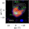 |
Fig. 7 Comparison of the PN N = 2–1 and HDCO J = 2–1 flux distributions. The PN N = 2–1 line flux (colourscale and bluecontours) is integrated in the velocity interval [−11;+4.6] km s−1; the first contour and contour interval are 3σ (2.8 × 10⁻² Jy beam−1 km s−1) and 2σ (1.8 × 10⁻² Jybeam−1 km s−1), respectively. The synthesized beam of the PN N = 2–1 is depicted by a blue ellipse in the bottom right corner. The HDCO J = 41,4−31,3 emission (white contours) is integrated in the velocity interval [−0.7;+3.4] km s−1; the first contour and contour interval are 20% and 15% of the peak intensity, respectively. The map was smoothed down to the angular resolution of the PN N = 2–1 line. The HDCO J = 2–1 data are from Fontani et al. (2014). Coordinates are in arcsecond offsets with respect to the nominal position of L1157-B1. |
4.2 Comparison with astrochemical models
The nature of the main P-carrier on dust grains is poorly constrained. In practice, P-chemistry shock models such as that of Aota & Aikawa (2012) consider two possibilities for the initial form and abundance of phosphorus. In the first case, phosphorus is considered to be locked onto dust grains mainly in the form of phosphine (PH3; Aota & Aikawa 2012). In the second case, phosphorus is considered to be locked into dust grains and is then desorbed into its atomic form to the gas phase at the passage of the shock.
In the first case, once dust is sputtered and enriches the gas phase, if the temperature is higher than ~100 K, PH3 reacts with H thanks to reactions with activation barriers higher than 300 K to form first PH2, then PH, and ultimately P (Aota & Aikawa 2012). The timescale for this process is relatively fast, that is, less than 1000 yr, according to the astrochemical models of Aota & Aikawa (2012) and Jiménez-Serra et al. (2018). Therefore, in both cases, although at different timescales, shocked gas is enriched in atomic P, which in turn is expected to react with H3O+ to form HPO+ in a first step and then PO. Alternative routes leading to PO are the reactions of P+ with H2 (Rivilla et al. 2016) and PH and PH2 with atomic O (Jiménez-Serra et al. 2018). The latter authors proposed that PO could also form efficiently through the reaction P + OH → PO + H in the high-temperature region of shocks. García de la Concepción et al. (2021) recently calculated the rate constant of this reaction and showed that it could represent an important route of PO formation in shock conditions, while accounting for the values of the PO/PN ratio reported observationally.
As in the case of PN, its formation depends on the amount of atomic N present in the gas phase. Two pathways have been proposed, the first one considers the reaction of PH, a product of phosphine degradation, with atomic N: PH + N → PN + H, while the second one considers the reaction PO + N → PN + O, as reported in the L1157 chemical models by Aota & Aikawa (2012) and Lefloch et al. (2016). Recent models proposed that PN could be destroyed by atomic O in a process leading to the formation of NO (PN + O → P + NO), which would become efficient in high-temperature regions of shocks (Souza et al. 2021), as in the jet impact region, which Herschel found to be associated with hot CO and OI emission (Benedettini et al. 2012).
The different PO/PN ratios measured across B1 confirm that the chemistry of phosphorus is time-dependent. This possibility was already proposed by Bergner et al. (2022) in their study of B1-a. Thanks to the accurate precession model of the L1157 outflow, the association of PN with the B1 apex allows us to set an upper limit of ~1700 yr on the age of the PN gas, corresponding to the kinematical age of the B1 region. This in turn allows us to constrain the timescale of the astrochemical modelling of L1157-B1 by Aota & Aikawa (2012), where PN does not reach abundances of greater than 10−9 before 104 yr, as well as those by Lefloch et al. (2016), where these values are reached but at a few 102 yr. Conversely, the PO abundance decreases in the gas phase and the PO/PN ratio becomes less than 1 after a few 100 yr. Progress has been made in the shock modelling of p-chemistry. In the recent model of the L1157-B1 shock of García de la Concepción et al. (2021), PN presents an abundance of almost 10−10 at the beginning of the shock and increases steadily until timescales of ≥400 yr when it reaches a constant abundance of ~10−9. These timescales are consistent with the age of the B1 apex (upper limit of ~1700 yr). However, PO only becomes more abundant than PN in the post-shock region for timescales of between a few decades and 200 yr (with an abundance of a few 10−9). This is consistent with the line profiles of PN and PO observed at the peak of the PN distribution (see Fig. 3), for which the terminal velocities of the PO emission (between −10 and 0 km s−1) fall within the terminal velocities of the PN emission (between −20 and 4 km s−1). The observed PN and PO line profiles could therefore reflect the internal chemical structure of the shock as predicted by the models of García de la Concepción et al. (2021).
We note that the modelling of the chemistry at work in the chemically active L1157 outflow is very challenging, as a huge number of species show a dramatic variation in abundance (Bachiller et al. 2001; Lefloch et al. 2017, 2018). An interesting hint is provided by nitrogen. There are a priori several sources of atomic N: the first one is atomic nitrogen N stored onto the dust grains during the preshock phase, which is of critical duration; the second comes from the destruction of NH3 into N, a reaction which comes into play as soon as the kinetic temperature rises above 3500 K; and a third pathway is the thermal dissociation of N2, which occurs at temperatures above 4000 K (Douglas et al. 2022). The atomic nitrogen in the high temperature shocked gas can react to form PN following the reaction PO + N → PN + O, but it can also create nitrogen oxide through the reaction OH + N → NO + H (e.g. Aota & Aikawa 2012). As a consequence, we expect an increase in NO abundance at high velocity, where the high-temperature gas should mainly emit. We note that indeed Codella et al. (2018) detected NO emission towards L1157-B1 in the context of the ASAI IRAM 30m project. An enhancement of the NO abundance of up to 6 × 10⁻⁶ has been measured, showing that the NO production increases in shocks. More specifically, NO has been found to trace the B1 low-velocity extended cavity. However, the NO spectra observed towards L1157-B1 clearly show an additional weaker component emitting at high velocity, between −6 km s−1 and −10 km s−1 (see Figs. 5 and 6 by Codella et al. 2018). This could indeed correspond to the shocked gas where atomic nitrogen is enhanced, contributing to the formation of both PN and NO.
5 Conclusions
Maps of the PO J = 5/2–3/2 and PN N = 2–1 emission lines obtained with the NOEMA interferometer at 3.4″ and 4.5″ × 3.6″ angular resolution, respectively, provide us with a detailed view of the spatial distribution of those species in the shock region L1157-B1. We find clear evidence that both species are tracing the apex of the bowshock only. Our analysis of the gas kinematics reveals that PN traces two different physical components, one associated with the apex and the bowshock, and the other one associated with the jet-impact shock region. Our comparison with the spatial distribution of well-known shock tracers leads us to the conclusion that both PO and PN are formed through gas-phase processes from a mother species located on dust grains: Firstly, the spatial distribution of their emissions are closely associated with those of SiO, and are formed through gas-phase processes. Secondly, a spatial anti-correlation is observed with the emission of HDCO, which traces the early regions of the shock, where the dust grains are sputtered.
PO is detected in a younger region (140 years earlier) of the shock than PN, implying that PO appears in the shocked gas phase before PN. Conversely, PN is detected in the southernmost and older regions of the shock, where PO is not detected, implying that PO disappears in the post-shocked gas before PN. We measured the abundance ratio PO/PN across the apex, and find it to increase from 2.9 to 4.7 between the older shock B1c and the younger shock B1a, separated by 140 yr. Such values are in agreement with those reported in studies of other star-forming regions (Rivilla et al. 2016; Bergner et al. 2019). These observations are consistent with the chemical scenario based on Aota & Aikawa (2012) and proposed by Lefloch et al. (2016), in which PO first forms in the gas phase, and quickly reacts in the gas phase to form PN. This scenario leads to smaller PO/PN ratios in older shocks.
The recent progress in the modelling of P-chemistry as well as the complexity of these networks require observational constraints. In particular, high-angular-resolution observations of NO as well as a more accurate view of the excitation conditions of P-bearing species with NOEMA would be extremely helpful, allowing us to better understand the pathways involved in the formation and the evolution of PO and PN.
Acknowledgements
We warmly thank the anonymous referee for their instructive comments and suggestions. Based on observations carried out under project number W16AI with the IRAM NOEMA Interferometer. IRAM is supported by INSU/CNRS (France), MPG (Germany) and IGN (Spain). B.L., C.Co., C.V., S.V. and C.Ce. acknowledge support from the European Unionâ Horizon 2020 research and innovation program under the Marie Sklodowska-Curie grant agreement no. 811312 for the project “Astro-Chemical Origins” (ACO) and the European Research Council (ERC) under the European Unionâ Horizon 2020 research and innovation program for the Project “The Dawn of Organic Chemistry” (DOC) grant agreement no. 741002. C.Co. and L.Po. acknowledge the PRIN-INAF 2016 The Cradle of Life – GENESIS-SKA (General Conditions in Early Planetary Systems for the rise of life with SKA), the PRIN-MUR 2020 MUR BEYOND-2p (Astrochemistry beyond the second period elements, Prot. 2020AFB3FX), the project ASI-Astrobiologia 2023 MIGLIORA (Modeling Chemical Complexity, F83C23000800005), the INAF-GO 2023 fundings PROTO-SKA (Exploiting ALMA data to study planet forming disks: preparing the advent of SKA, C13C23000770005), and the INAF Mini-Grant 2022 ÒChemical OriginsÓ (PI: L. Podio). I.J.-S. acknowledges support from grant no. PID2019-105552RB-C41 by the Spanish Ministry of Science and Innovation/State Agency of Research MCIN/AEI/10.13039/501100011033.
References
- Altwegg, K., Balsiger, H., Bar-Nun, A., et al. 2016, Sci. Adv., 2, 1600285 [CrossRef] [Google Scholar]
- Anders, E., & Grevesse, N. 1989, Geochim. Cosmochim. Acta, 53, 197 [Google Scholar]
- Aota, T., & Aikawa, Y. 2012, ApJ, 761, 74 [NASA ADS] [CrossRef] [Google Scholar]
- Asplund, M., Grevesse, N., & Sauval, A. J. 2009, ARA&A, 47, 481 [NASA ADS] [CrossRef] [Google Scholar]
- Ayala, S., Noriega-Crespo, A., Garnavich, P. M., et al. 2000, AJ, 120, 909 [NASA ADS] [CrossRef] [Google Scholar]
- Bachiller, R. 1996, ARA&A, 34, 111 [NASA ADS] [CrossRef] [Google Scholar]
- Bachiller, R., Pérez-Gutiérrez, M., Kumar, M. S. N., et al. 2001, A&A, 372, 899 [NASA ADS] [CrossRef] [EDP Sciences] [Google Scholar]
- Bally, J. 2016, ARA&A, 54, 491 [Google Scholar]
- Benedettini, M., Viti, S., Codella, C., et al. 2007, MNRAS, 381, 1127 [Google Scholar]
- Benedettini, M., Busquet, G., Lefloch, B., et al. 2012, A&A, 539, A3 [NASA ADS] [CrossRef] [EDP Sciences] [Google Scholar]
- Benedettini, M., Viti, S., Codella, C., et al. 2013, MNRAS, 436, 179 [Google Scholar]
- Bergner, J. B., Öberg, K. I., Walker, S., et al. 2019, ApJ, 884, L36 [CrossRef] [Google Scholar]
- Bergner, J. B., Burkhardt, A. M., Öberg, K. I., et al. 2022, ApJ, 927, 7 [NASA ADS] [CrossRef] [Google Scholar]
- Bernal, J. J., Koelemay, L. A., & Ziurys, L. M. 2021, ApJ, 906, 55 [NASA ADS] [CrossRef] [Google Scholar]
- Cabrit, S., Raga, A., & Gueth, F. 1997, in Herbig-Haro Flows and the Birth of Stars; IAU Symposium No. 182, eds. B. Reipurth & C. Bertout (Kluwer Academic Publishers) 163 [CrossRef] [Google Scholar]
- Cazzoli, G., Claudi, L., & Puzzarini, C. 2006, JMoSt., 780, 260 [NASA ADS] [Google Scholar]
- Ceccarelli, C., Caselli, P., Fontani, F., et al., 2017, ApJ, 850, 176 [NASA ADS] [CrossRef] [Google Scholar]
- Cernicharo, J. 2012, EAS, 58, 251 [NASA ADS] [CrossRef] [EDP Sciences] [Google Scholar]
- Chini, R., Ward-Thompson, D., Kirk, J. M., et al. 2001, A&A, 369, 155 [NASA ADS] [CrossRef] [EDP Sciences] [Google Scholar]
- Codella, C., Cabrit, S., Gueth, F., et al. 2007, A&A, 462, A53 [Google Scholar]
- Codella C., Cabrit, S., Gueth, F., et al. 2014, A&A, 568, A5 [NASA ADS] [CrossRef] [EDP Sciences] [Google Scholar]
- Codella, C., Ceccarelli, C., Caselli, P., et al. 2017, A&A, 605, A3 [NASA ADS] [CrossRef] [EDP Sciences] [Google Scholar]
- Codella, C., Viti, S., Lefloch, B., et al. 2018, MNRAS, 474, 5694 [NASA ADS] [CrossRef] [Google Scholar]
- Crimier, N., Ceccarelli, C., Alonso-Albi, T., et al. 2010, A&A, 516, A102 [NASA ADS] [CrossRef] [EDP Sciences] [Google Scholar]
- Douglas, K. M., Gobrecht, D., & Plane, J. M. C. 2022, MNRAS, 515, 99 [NASA ADS] [CrossRef] [Google Scholar]
- Eisloeffel, J., Smith, M. D., Davis, C. J., & Ray, T. P. 1996, AJ, 112, 2086 [NASA ADS] [CrossRef] [Google Scholar]
- Ferrero, L. V., Gómez, M., & Gunthard, G. 2015, BAAA, 57, 126 [NASA ADS] [Google Scholar]
- Flower, D. R., & Pineau des Forêts, G. 2003, MNRAS, 343, 390 [Google Scholar]
- Fontani, F., Codella, C., Ceccarelli, C., et al. 2014, ApJ, 788, L43 [Google Scholar]
- Fontani, F., Rivilla, V. M., Caselli, P., et al. 2016, ApJ, 822, L30 [NASA ADS] [CrossRef] [Google Scholar]
- Fontani, F., Rivilla, V. M., van der Tak, F. F. S., et al. 2019, MNRAS, 489, 4530 [CrossRef] [Google Scholar]
- García de la Concepción, J., Puzzarini, C., Barone, V. V., et al. 2021, ApJ, 922, 169 [CrossRef] [Google Scholar]
- Gómez-Ruiz, A. I., Codella, C., Lefloch, B., et al. 2015, MNRAS, 446, 3346 [Google Scholar]
- Gueth, F., Guilloteau, S., & Bachiller, R. 1996, A&A, 307, 891 [NASA ADS] [Google Scholar]
- Gueth, F., Guilloteau, S., Bachiller, R. 1998, A&A, 333, 287 [NASA ADS] [Google Scholar]
- Gusdorf, A., Pineau Des Forêts, G., Cabrit, S., & Flower, D. R. 2008, A&A, 490, 695 [NASA ADS] [CrossRef] [EDP Sciences] [Google Scholar]
- Gusdorf, A., Riquelme, D., Anderl, S., et al. 2015, A&A, 575, A98 [CrossRef] [EDP Sciences] [Google Scholar]
- Gusdorf, A., Anderl, S., Lefloch, B., et al. 2017, A&A, 602, A8 [NASA ADS] [CrossRef] [EDP Sciences] [Google Scholar]
- Hara, C., Kawabe, R., Nakamura, F., et al. 2021, ApJ, 912, 34 [NASA ADS] [CrossRef] [Google Scholar]
- Hirth, G. A., Mundt, R., Solf, J., & Ray, T. P. 1994, ApJ, 427, L99 [NASA ADS] [CrossRef] [Google Scholar]
- Jiménez-Serra, I., Viti, S., Quenard, D., & Holdship, J. 2018, ApJ, 862, 128 [CrossRef] [Google Scholar]
- Jura, M., & York, D. G. 1978, ApJ, 219, 861 [NASA ADS] [CrossRef] [Google Scholar]
- Karnath, N., Prchlik, J. J., Gutermuth, R. A., et al. 2019, ApJ, 871, 46 [NASA ADS] [CrossRef] [Google Scholar]
- Kawaguchi, K., Saito, S., & Hirota, E. 1983, JChPh, 79, 629 [NASA ADS] [Google Scholar]
- Lefèvre, C., Cabrit, S., Maury, A. J., et al. 2017, A&A, 604, L1 [CrossRef] [EDP Sciences] [Google Scholar]
- Lefloch, B., Eisloeffel, J., & Lazareff, B. 1996, A&A, 313, L17 [NASA ADS] [Google Scholar]
- Lefloch, B., Cernicharo, J., Rodríguez, L. F., et al. 2002, ApJ, 581, 335 [NASA ADS] [CrossRef] [Google Scholar]
- Lefloch, B., Cabrit, S., Busquet, G., et al. 2012, ApJ, 757, L25 [Google Scholar]
- Lefloch, B., Vastel, C., Viti, S., et al. 2016, MNRAS, 462, 3937 [CrossRef] [Google Scholar]
- Lefloch, B., Ceccarelli, C., Codella, C., et al. 2017, MNRAS, 469, L73 [Google Scholar]
- Lefloch, B., Bachiller, R., Ceccarelli, C., et al. 2018, MNRAS, 477, 4792 [Google Scholar]
- Leurini, S., Codella, C., Lopez-Sepulcre, A., et al. 2014, A&A, 570, A49 [NASA ADS] [CrossRef] [EDP Sciences] [Google Scholar]
- López-Sepulcre, A., Balucani, N., Ceccarelli, C., et al. 2019, ACS Earth Space Chem., 3, 2122 [CrossRef] [Google Scholar]
- Louvet, F., Motte, F., Gusdorf, A., et al. 2016, A&A, 595, A122 [NASA ADS] [CrossRef] [EDP Sciences] [Google Scholar]
- Macía, E. 2005, Chem. Soc. Rev., 34, 691 [CrossRef] [Google Scholar]
- Maret, S., Bergin, E. A., Neufeld, D. A., et al. 2009, ApJ, 698, 1244 [NASA ADS] [CrossRef] [Google Scholar]
- May, P. W., Pineau des Forêts, G., Flower, D. R., et al. 2000, MNRAS, 318, 809 [NASA ADS] [CrossRef] [Google Scholar]
- Mininni, C., Fontani, F., Rivilla, V. M., et al. 2018, MNRAS, 476, L39 [CrossRef] [Google Scholar]
- Müller, H. S. P., Schlöder, F., Stutzki, J., et al. 2005, JMoSt., 742, 215 [Google Scholar]
- Podio, L., Codella, C., Gueth, F., et al. 2016, A&A, 593, A4 [NASA ADS] [CrossRef] [EDP Sciences] [Google Scholar]
- Podio, L., Codella, C., Lefloch, B., et al. 2017, MNRAS, 470, L16 [Google Scholar]
- Podio, L., Tabone, B., Codella, C., et al. 2021, A&A, 648, A45 [NASA ADS] [CrossRef] [EDP Sciences] [Google Scholar]
- Raga, A., & Cabrit, S. 1993, A&A, 278, 267 [Google Scholar]
- Rimola, A., Skouteris, D., Balucani, N., et al. 2018, ACS Earth Space Chem., 2, 720 [Google Scholar]
- Ridgway, S. T. 1974, Bull. Am. Astron. Soc., 6, 376 [Google Scholar]
- Rivilla, V. M., Fontani, F., Beltrán, M., I., et al. 2016, ApJ, 826, 161 [CrossRef] [Google Scholar]
- Rivilla, V. M., Jiménez-Serra, I., Zeng, S., et al. 2018, MNRAS, 475, 30 [Google Scholar]
- Rivilla, V. M., Drozdovskaya, M. N., Altwegg, K., et al. 2020, MNRAS, 492, 1180 [Google Scholar]
- Skouteris, D., Vazart, F., Ceccarelli, C., et al. 2017, MNRAS, 468, L1 [NASA ADS] [Google Scholar]
- Souza, A. C., Silva, M. X., & Galvão, B. G. 2021, MNRAS, 507, 1899 [NASA ADS] [CrossRef] [Google Scholar]
- Tafalla, M., Santiago-García, J., Hacar, A., & Bachiller R. 2010, A&A, 522, A91 [NASA ADS] [CrossRef] [EDP Sciences] [Google Scholar]
- Tobola, R., Klos, J., Lique, F., et al. 2007, A&A, 468, 1123 [NASA ADS] [CrossRef] [EDP Sciences] [Google Scholar]
- Turner, B. E., Tsuji, T., & Bally, J. 1990, ApJ, 365, 569 [NASA ADS] [CrossRef] [Google Scholar]
- Vastel, C., Bottinelli, S., Caux, E., et al. 2015, SF2A-2015: Proceedings of the Annual meeting of the French Society of Astronomy and Astrophysics, eds. F. Martins, S. Boissier, V. Buat, L. Cambrésy, P. Petit, 313 [Google Scholar]
- Zucker, C., Speagle, J. S., Schlafly, E. F., et al. 2019, ApJ, 879, 125 [NASA ADS] [CrossRef] [Google Scholar]
All Tables
PN and PO lines observed with the IRAM NOEMA interferometer in the D configuration.
Column densities of PN and PO determined at the shock positions B1a and B1c and at the emission peaks of the PN N = 2–1 and PO 2Π1/2 J = 5/2–3/2 e 3–2 (108998 MHz) lines.
All Figures
|
Fig. 1 Phosphorus-bearing molecules in the L1157-B1 protostellar shock. Left: emission map of the PN N = 2–1 line obtained with NOEMA in the southern lobe of the L1157 outflow. The emission (colour) is integrated in the velocity range −10 to +5 km s−1. The first contour and contour interval (blue) are 3σ (36 mJy beam−1 km s−1) and 2σ, respectively. The dashed white circle shows the primary beam of the PN image (53″). The CO J = 1–0 outflow emission, as imaged by Gueth et al. (1996) is superimposed in white contours. The white triangle at the top points to the position of the L1157-mm protostar. Right: magnified view of the L1157-B1 central region. The maps are centred at: α(J2000) = 20h39m 10s.2, δ(J2000) = +68°01′10.″5. The PN N = 2–1 map is compared with the stacked intensity distribution of PO J = 5/23/2, F = 3–2, ef (cyan thick contours). The first contour and contour interval of the PO map are 3σ (21 mJy beam−1 km s−1) and 2σ respectively. The 3σ level of the p-H2CO J = 20,2−10,1 integrated emission (Benedettini et al. 2013; grey contours) is here used to define the whole structure of the B1 shock. The cyan ellipse draws the synthesised beam of the PO observations, and shock knots B1a-B1b-B1c-B0e are marked by yellow triangles. |
| In the text | |
|
Fig. 2 Top: comparison in flux density scale between the PN and PO spectra as observed using the IRAM 30 m antenna (magenta, Lefloch et al. 2016) and that extracted from the NOEMA map (black) from a circular region equal to the IRAM 30m HPBW. Top: PN N= 2–1 spectra. The HPBW is 26″.2. The vertical dot-dashed line marks the systemic velocity of L1157-mm (V = +2.7 km s−1). The blue lines indicate the frequencies of the ΔJ = 0, ±1 transitions of the N = 2–1 pattern (see Table 1). Middle: same as in the top panel but for the PO 2Π1/2 J = 5/2–3/2 F = 3–2 f transition (IRAM 30 m beam: 22″.6). Bottom: same as in the middle panel but for the PO transition 2Π1/2 J = 5/2–3/2 F = 3–2 e. |
| In the text | |
|
Fig. 3 Spatial distribution of the PN N = 2–1 emission as a function of velocity, as observed with NOEMA, between −14 km s−1 and +7.4 km s−1. Each velocity channel has a width of 2 km s−1. The velocity is marked in red in the top left corner of each panel. The synthesised beam is depicted by a blue ellipse in the bottom right corner. First contour and contour interval (in blue) are 3σ and 1σ of the flux distribution, respectively. The location of the shock knots B1a-B1c and B0e are marked by green crosses. |
| In the text | |
|
Fig. 4 PN and PO spectra. Top: PN N = 2–1 spectrum at the peak of the PN spatial distribution. The vertical dot-dashed line marks the systemic velocity of L1157-mm. Bottom: PO emission at the peak of the spatial distribution obtained by stacking the lines 2Π1/2 J = 5/2–3/2, F = 3–2 f and 2Π1/2 J = 5/2–3/2 F = 3–2 e. Intensities are expressed in TB scale. |
| In the text | |
|
Fig. 5 Comparison of the PN N = 2–1 and SiO J = 2–1 line emissions. Left: high-velocity range. The PN N = 2–1 line flux (colourscale and red contours) is integrated in the velocity interval [−11;−5.3] km s−1; the first contour and contour interval are 3σ (1.8 × 10⁻² Jy beam−1 km s−1) and 2σ (1.2 × 10⁻² Jy beam−1 km s−1), respectively. The SiO J = 2–1 emission (white contours) is integrated in the velocity interval [−19.7;−6.7] km s−1; the first contour and contour interval are 20% and 15% of the SiO peak intensity, respectively. Right: low-velocity range. The PN N = 2–1 line flux is integrated in the velocity interval [−5.3;+4.6] km s−1; the first contour and contour interval are 3σ (2.5 × 10⁻² Jy beam−1 km s−1) and 2σ (1.6 × 10⁻² Jy beam−1 km s−1), respectively. The SiO J = 2–1 emission is integrated in the velocity interval [−6.7; +3.7] km s−1; the first contour and contour interval are 20% and 15% of the SiO peak intensity, respectively. The red and white ellipses depict the synthesised beams of the PN N = 2–1 and SiO J = 2–1 observations, respectively. Coordinates are in arcsecond offsets with respect to the nominal position of B1. |
| In the text | |
|
Fig. 6 PN N = 2–1 emission detected with NOEMA towards shock positions B1a (top) and B1c (bottom). Line intensities are expressed in TB scale. The vertical red dashed line marks the systemic velocity of L1157-mm. The horizontal black dashed line marks the 1σ noise level of the spectrum (12 mK). |
| In the text | |
|
Fig. 7 Comparison of the PN N = 2–1 and HDCO J = 2–1 flux distributions. The PN N = 2–1 line flux (colourscale and bluecontours) is integrated in the velocity interval [−11;+4.6] km s−1; the first contour and contour interval are 3σ (2.8 × 10⁻² Jy beam−1 km s−1) and 2σ (1.8 × 10⁻² Jybeam−1 km s−1), respectively. The synthesized beam of the PN N = 2–1 is depicted by a blue ellipse in the bottom right corner. The HDCO J = 41,4−31,3 emission (white contours) is integrated in the velocity interval [−0.7;+3.4] km s−1; the first contour and contour interval are 20% and 15% of the peak intensity, respectively. The map was smoothed down to the angular resolution of the PN N = 2–1 line. The HDCO J = 2–1 data are from Fontani et al. (2014). Coordinates are in arcsecond offsets with respect to the nominal position of L1157-B1. |
| In the text | |
Current usage metrics show cumulative count of Article Views (full-text article views including HTML views, PDF and ePub downloads, according to the available data) and Abstracts Views on Vision4Press platform.
Data correspond to usage on the plateform after 2015. The current usage metrics is available 48-96 hours after online publication and is updated daily on week days.
Initial download of the metrics may take a while.