| Issue |
A&A
Volume 681, January 2024
|
|
|---|---|---|
| Article Number | A37 | |
| Number of page(s) | 10 | |
| Section | Astrophysical processes | |
| DOI | https://doi.org/10.1051/0004-6361/202245251 | |
| Published online | 05 January 2024 | |
Laboratory modeling of YSO jets collimation by a large-scale divergent interstellar magnetic field
1
IAP – A.V. Gaponov-Grekhov Institute of Applied Physics, Russian Academy of Sciences,
603950
Nizhny Novgorod,
Russia
e-mail: This email address is being protected from spambots. You need JavaScript enabled to view it.
2
Joint Institute for High Temperatures, RAS,
125412
Moscow,
Russia
3
LULI – CNRS, CEA, UPMC Univ Paris 06: Sorbonne Université, École Polytechnique, Institut Polytechnique de Paris,
91128
Palaiseau Cedex,
France
4
INASAN – Institute of Astronomy, Russian Academy of Sciences,
119017
Moscow,
Russia
5
NCPhM – National Center for Physics and Mathematics,
Sarov,
Russia
6
Sorbonne Université, Observatoire de Paris, PSL Research University, LERMA,
CNRS UMR 8112,
75005
Paris,
France
Received:
19
October
2022
Accepted:
19
October
2023
Abstract
Context. Numerical studies as well as scaled laboratory experiments suggest that bipolar outflows arising from young stellar objects (YSOs) could be collimated into narrow and stable jets as a result of their interaction with a poloidal magnetic field. However, this magnetic collimation mechanism was demonstrated only for the simplified topology of the uniform poloidal magnetic field.
Aims. We have extended the experimental studies to the case of a plasma outflow expanding in a region of strong poloidal magnetic field and then propagating through divergent magnetic field lines. In this case the magnetic field distribution is closer to the hourglass magnetic field distribution expected near YSOs. Our aim was to find out whether (and under what conditions) magnetic collimation is possible in such a strongly nonuniform B-field configuration.
Methods. The experiments were carried out on the PEARL high-power laser facility. The laser produced plasma outflow was embedded in a strong (~10T) magnetic field generated by our unique magnetic system. The morphology and dynamics of the plasma were diagnosed with a Mach-Zehnder interferometer.
Results. Laboratory experiments and 3D numerical modeling allow us to reveal the various stages of plasma jet formation in a divergent poloidal magnetic field. The results show (i) that there is a fundamental possibility for magnetic collimation of a plasma outflow in a divergent magnetic field; (ii) that there is good scalability of astrophysical and laboratory flows; (iii) that the conditions for the formation of a magnetic nozzle, hence collimation by poloidal magnetic field, have been met; and (iv) that the propagation of the jet proceeds unimpeded through the region of weak and strongly divergent magnetic fields, maintaining a high aspect ratio.
Conclusions. Since we have verified that the laboratory plasma scales favorably to YSO jets and outflows, our laboratory modeling hints at the possibility of the YSO jet collimation in a divergent poloidal magnetic field.
Key words: stars: jets / stars: pre-main sequence / ISM: jets and outflows
© The Authors 2024
 Open Access article, published by EDP Sciences, under the terms of the Creative Commons Attribution License (https://creativecommons.org/licenses/by/4.0), which permits unrestricted use, distribution, and reproduction in any medium, provided the original work is properly cited.
This article is published in open access under the Subscribe to Open model. This email address is being protected from spambots. You need JavaScript enabled to view it. to support open access publication.
1 Introduction
Jets are commonly observed in accreting young stellar objects (YSO). Such collimated supersonic outflows are observed over a wide range of radiation wavelengths (from millimeter waves to X-rays) at the early stages of star formation (YSO classes I and II; Bally et al. 2007; Ray et al. 1990; Anglada et al. 2018), when matter is actively accreted onto the star. Jets are usually observed along the rotation axis of a protostar-accretion disk system (Anathpindika & Whitworth 2008; Kamali et al. 2019), and they are believed to play a key role in the evolution of YSO’s (Pudritz et al. 2007; Königl & Salmeron 2010).
Gaining a comprehensive understanding of the early stages of star formation requires a grasp of the underlying physical processes that lead to the formation of jets and their distinct morphology. This knowledge is crucial to understand how angular momentum is extracted from the system and how mass is accreted.
The mechanisms of the generation of outflows and their col-limation into jets are still not fully understood and are being actively discussed. To date, a number of different outflow launching models have been proposed in the literature (e.g., Ferreira et al. 2006, 2002; Blandford & Payne 1982; Matt & Pudritz 2005; Goodson et al. 1999). It is generally accepted that the matter source of a jet is located in the central part of a YSO, including the protostar and the accretion disk, and the models describing the outflow generation from this area are often called “central wind” models. For example, some observational (Edwards et al. 2003, 2006; Dupree et al. 2005) and numerical (Kwan et al. 2007; Matt & Pudritz 2008) works point to the presence of powerful stellar winds in YSOs. Disk wind models where outflows are magneto-centrifugally driven are also very popular, for example extended disk winds (Blandford & Payne 1982; Ferreira 1997) and X-winds (Shu et al. 1994).
Further propagation of the plasma outflow and its collimation leading in some cases to surprisingly narrow and stable jets are described by a number of completely different (and sometimes controversial) models. Some models (Blandford & Payne 1982; Bellan 2018) show that the outflow can be self-collimated by a toroidal magnetic field at the launching stage; however, these models often demonstrate unstable jets to the kink magnetohy-drodynamic (MHD) instabilities (Moll et al. 2008; Moll 2009; Spruit et al. 1997; Ciardi et al. 2007; Begelman 1998). The differential rotation of outflows originating in the Keplerian disk gives a stabilizing effect, but does not completely exclude the development of an instability (Moll et al. 2008; Moll 2009). However, as follows from a number of works (Wright 1973; Spruit et al. 1997), a stable jet can exist if a mixed poloidal-toroidal magnetic field is included. Stable large-scale jets whose characteristics (e.g., collimation angle, velocity, power to accretion luminosity of YSOs) are in a good agreement with YSO observations could be successfully reproduced in simulations relying on MHD colli-mation by a poloidal magnetic field (Matt et al. 2003; Albertazzi et al. 2014; Ustamujic et al. 2018). The mechanism of such a col-limation was studied in our earlier works, not only theoretically (Ciardi et al. 2013), but also in the course of several laboratory experiments (Albertazzi et al. 2014; Higginson et al. 2017; Revet et al. 2021; Korobkov et al. 2023). To perform these experiments, a laser-produced high-velocity plasma plume was formed inside pulsed Helmholtz coils with a magnetic field of up to 10-30 T. It was shown both experimentally and numerically that a stable and narrow jet can be formed entirely due to the effect of a uniform poloidal magnetic field as a result of the collimation of an initially wide-angle plasma flow by the magnetic nozzle (Higginson et al. 2017; Revet et al. 2021).
However, the real structure of the large-scale magnetic field near a YSO differs significantly from the idealized picture of a uniform poloidal magnetic field. Astronomical observations based on polarization measurements of molecular and dust radiation (Schleuning 1998; Girart et al. 1999, 2006; Lai et al. 2002; Kwon et al. 2019; Hull et al. 2020) give a hint that the structure of the magnetic field near the YSO has an hourglass morphology compressed in the direction of the protostar by the accretion matter (shown schematically in the left panel of Fig. 1). In addition, this structure often appears in full-scale magnetohydrodynamic simulations of the disk (Allen et al. 2003; Li & Cao 2019; Zhu & Stone 2017; Jacquemin-Ide et al. 2021). In other words, the magnetic field in the vicinity of the accretion disk is divergent and inhomogeneous, and the plasma outflow is streaming from the region of the strong magnetic field along divergent magnetic field lines.
In this paper, we study experimentally the expansion of a wide-angle super-magnetosonic flow in an inhomogeneous magnetic field with diverging field lines. Despite the interest in the problem of jet formation, this has not yet been explored in detail in laboratory experiments, due to the significant technical difficulties associated with the creation of highly inhomogeneous multi-Tesla magnetic fields; the need to use such strength for the magnetic field will be justified below. This is now possible using our unique reinforced magnetic system (see Luchinin et al. 2021 for details).
The paper is organized as follows. In Sect. 2, we describe the laboratory setup. In Sect. 3, we present the topology of plasma outflows and discuss the parameters of the laboratory plasma. In Sect. 4, we demonstrate the scalability of the laboratory experiment to the ideal MHD model of YSO jets. In Sect. 5, we present the results of the full-scale numerical hybrid (PIC-fluid) simulations of the laboratory setup. In Sect. 6, we discuss the results and draw our conclusions.
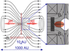 |
Fig. 1 Modeling setup. Left: schematic representation of the large-scale structure of the interstellar magnetic field disturbed by the accretion disk of a young stellar object (YSO) and taking the shape of an hourglass. The structure of the magnetic fields in the figure is an example and not a complete match. The red arrows indicate axisymmetric jets. The blue rectangle shows the area modeled in the experiment. Right: schematic of the experiment indicating the magnetic field structure with a plasma outflow. The shaded areas are unavailable for diagnostics; the white area illustrates the diagnostic window. |
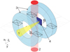 |
Fig. 2 Schematic view of the experimental setup. 1 – Nanosecond heating laser pulse, 2 – Femtosecond laser probe pulse, 3 – Windings, 4 – Teflon target. |
2 Experimental setup
The experiments were conducted on the PEARL high-power laser facility (IAP RAS; Lozhkarev et al. 2007; Ginzburg et al. 2021; Soloviev et al. 2022). In our previous works, (Burdonov et al. 2021, 2022; Soloviev et al. 2021) we performed several experiments on laboratory astrophysical modeling at the PEARL laser facility, and additional technical details can be found there. The specific conditions that are unique and important to the current experiment are discussed below. The experimental setup is shown in Fig. 2.
An optical laser pulse with an energy of around 10 J and a FWHM duration of 1 ns at a wavelength of 527 nm was focused on the surface of a Teflon (CF2) target. To focus the laser radiation, a lens with a focal length of 1 m was used, which provided a spot of about 0.35 mm in diameter on the target surface. This arrangement made it possible to have an intensity of the laser radiation on the target surface on the order of 1013 Wcm−2. The irradiation of the target with a nanosecond laser pulse led to the ablation of matter from the target surface and the formation of a supersonic (~200−300 kms−1) plasma flow expanding into vacuum along z, which is the main expansion axis. In the close vicinity of the target the initial plasma flow morphology is conical with an opening angle of around 40° (Revet 2018). The plasma temperature measured in similar conditions using a X-ray focusing spectrometer with spatial resolution (FSSR; Faenov et al. 1994) was about 100 eV near the target surface and decreased to 30 eV at a distance on the order of a few centimeters from the target (Higginson et al. 2017). To study the process of the interaction of plasma outflows with a poloidal magnetic field, a Teflon target was placed inside the magnetic system as is shown qualitatively in Fig. 2.
The magnetic system used in the experiments consisted of a pair of Helmholtz coils (Fig. 3) with its symmetry axis directed along the z-axis. The gap of 11 mm between the Helmholtz coils was used as a diagnostic window to observe the dynamics of plasma flows in the ambient magnetic field (see Figs. 1, right, and 2).
The coils of the magnetic system can be connected to the power supply in two different ways generating co-directed or oppositely directed currents in the coils. In the case of co-directed currents, a quasi-uniform magnetic field is generated in the center of the magnetic system (Fig. 4a). If the currents are directed oppositely, then a cusp magnetic field configuration is formed with a zero magnetic field in the center of the magnetic system (Fig. 4b). The structure of the magnetic field lines for both cases is presented in Figs. 4a and b along with 3D color maps of the magnetic induction inside the magnetic system. The profiles of the Bz-component of the magnetic field for both types of the connections are presented in Fig. 4c. The maximum induction of poloidal magnetic field in the present experiments was limited by 9 T due to the risk of rupture of the oppositely connected magnetic system by mechanical loads on its structural elements that reach up to 108 Nm−2 (Luchinin et al. 2021).
The plasma evolution was diagnosed with a Mach-Zehnder interferometer. The probing was done using a femtosecond laser pulse (10 mJ, 100 fs) which was synchronized with the nanosecond heating laser pulse. The delay line used to trace the evolution of the plasma flow made it possible to produce snapshots of the plasma with a delay of up to 100 ns after the start of laser irradiation of the target.
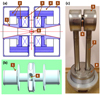 |
Fig. 3 Schematic sectional view of our magnetic system (a), the 3D model of the load-bearing metal frame (b), and a photo of the manufactured magnetic system (c). The numbers indicate the following: 1 - Load-bearing metal frame, 2 – Composite elements of the load-bearing frame, 3 – Windings, 4 – Nitrogen chamber, 5 – External shield, 6 – Conical holes for laser radiation input and plasma flow output, 7 – Channels for liquid nitrogen supply and placement of current leads, and 8 – Vacuum-tight bellows docking unit. The figure is from the article Luchinin et al. (2021), which presents the development of the magnetic system. |
 |
Fig. 4 Structure of the magnetic field: (a) co-directional connection of the coils, (b) oppositely directed connection, (c) Bz profiles on the axis of the magnetic system. |
3 Experimental approach and results
3.1 Collimation of a plasma jet via a poloidal quasi-uniform magnetic field
Although the main goal of this work is to study the morphology of plasma flows in a divergent hourglass-like magnetic field, in order to have a reference case to which the other configurations can be compared we began our studies with a series of experiments on plasma flow expansion into a uniform magnetic field. In this case the value of the quasi-uniform magnetic field B0 at the center of the magnetic system (see Fig. 4c) was chosen to be approximately equal to the maximum magnetic field of the cusp configuration. In addition, these experiments in a quasi-uniform magnetic field B0 allow us to study the initial stage of plasma expansion that occurs in the region of strong magnetic field in the cusp case. As shown in the right panel of Fig. 1, our diagnostic window is located in the central part of the magnetic system, and for the experiments with a cusp magnetic field, this region is not accessible to our diagnostics.
Based on our results and previous works (Ciardi et al. 2013; Albertazzi et al. 2014; Higginson et al. 2017) we can describe the plasma evolution and jet formation as follows. The plasma flow is launched thermally from the laser-irradiated region and expands at super-magnetosonic speeds. Because of its relatively high temperature, the plasma is highly conductive and the magnetic flux present in the plume when the plasma was formed is frozen into it. Since the expansion is supermagnetosonic, it sweeps and compresses the magnetic field, and thus modifies the initial distribution of the magnetic flux Ψ enclosed in a cylindrical circle with radius r (see numerical modeling in Sect. 5). The electron plasma distribution obtained from laser interferom-etry is presented in Fig. 5, which clearly shows the process of magnetic collimation of the initially diverging plasma flow.
The plasma flow expansion is initially (within 5 ns after irradiation) dominated by its kinetic energy (i.e., its ram pressure is higher than the magnetic pressure). The first stage of the magnetic collimation (Fig. 5a) corresponds to the deceleration of the plasma plume by the magnetic field, the formation of a dia-magnetic cavity, and the formation of a conical shock (diamond shock) structure at its apex. This standing shock leads to the re-focusing of the flow into a jet (Ciardi et al. 2013; Albertazzi et al. 2014; Higginson et al. 2017). The later evolution of the plasma flow are shown in Figs. 5b–d and correspond to the collapse of the cavity under the action of the magnetic forces (Fig. 5b). The collapse occurs because the generation of the plasma in the experiments is impulsive, so that the plasma flow ram pressure decreases in time.
The areal electron density measurements allows us to compare the characteristic radius of the plasma flow collimation with the deceleration radius in CGS units  , the scale on which a uniformly expanding cloud of conducting plasma with energy E is stopped by a uniform magnetic field B (Ciardi et al. 2013; Zakharov et al. 2006; Winske et al. 2019). For our parameters (E = 10 J, B = 9 T), we find Rb ~ 4 mm (i.e., a diameter 2Rb consistent with the observed diameter in Fig. 5a).
3.2 Expansion of a laser plasma into a diverging magnetic field
We now present the results of the expansion of the plasma flow into a diverging magnetic field. As described earlier, opposite currents in the coils were used to create a cusp magnetic field configuration (see Figs. 4b and c). The plasma flow in these experiments thus propagated from the region of strong magnetic field through diverging magnetic field lines toward the magnetic zero point. To study the influence, on the plasma flow morphology, of the length of the strong magnetic field region over which the plasma propagated, the laser-irradiated target was placed at different distances from the center of the magnetic system. The results are represented in Fig. 6 (at 28 and 48 ns after laser irradiation of the target) and Fig. 7 (at 68 ns after laser irradiation); the plasma flow morphology was imaged at the center of the magnetic system (i.e., in the vicinity ofthe magnetic zero point).
As expected, when the target was located in the close vicinity of the zero-point region the magnetic field had virtually no effect on the plasma dynamics, and the observed flow pattern was similar to the expansion without a magnetic field, which is a quasi-uniform diverging conical plasma flow with an opening angle of about 40° (see Figs. 6a, c and 7a). However, even a small displacement of the target into the position located at 9 mm from the zero point (Figs. 6b and 7b) already leads to a noticeable narrowing of the flow pattern.
Further displacement of the target inside one of the magnetic coils to the distance of 13.5 mm and more from the center of the magnetic system leads to the formation of well-collimated plasma flows propagating through the zero-point region (Figs. 6d and Figs. 7c–f). Such a strong change in the morphology of the plasma flow is caused by the fact that at the initial stage of its expansion the plasma flow interacts with a strong poloidal magnetic field.
Furthermore, based on these experimental results, we can determine the characteristic length of the strong magnetic field region that is required to collimate the plasma flow. Assuming that the magnetic field is strong when it exceeds |Bmax| / 2 = 4.5T (this point is located at z ≈ 7 mm from the magnetic zero point, see Fig. 4), the interaction length required for plasma flow collimation is found to be on the order of 9 mm.
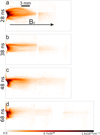 |
Fig. 5 Two-dimensional density profiles of the plasma stream propagating along a quasi-uniform magnetic field at 28 ns (a), 38 ns (b), 48 ns (c), and 68 ns (d) after the laser irradiation of the target. The spatial scale shown in (a) is the same for all the images. To demonstrate the evolution of the plasma cavity, the position of the target was shifted from shot to shot. Each panel in this figure is composed of a few such experimental snapshots. |
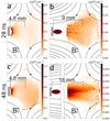 |
Fig. 6 Two-dimensional density profiles of the plasma stream propagating through a poloidal diverging magnetic field at 28 ns (a, b) and 48 ns (c, d) after laser irradiation of the target. The gray rectangle shows the location of the target. To depict the position of the target and reduce the scale of the picture, panel d is drawn with a gap, represented by the dashed line. |
3.3 Discussion of the experimental results
We have investigated the dynamics and topology of a plasma flow propagating in a diverging magnetic field under various initial conditions corresponding to different positions of the flow launching point with respect to the magnetic zero point. We have shown that the topology of the emerging flow depends significantly on whether the plasma flow launching point is located in the region of a strong poloidal magnetic field or, on the contrary, in the region of strongly divergent magnetic field.
The first important result revealed in Figs. 6 and 7 is that even a rather short region of a strong poloidal magnetic field of length H is enough to magnetically collimate a diverging plasma plume into a narrow jet. For the ~9 T magnetic field used in our experiments, the minimum length H of this strong-field region is approximately 9–10 mm, which corresponds to the target positions ≳13.5 mm from the center of the magnetic system (see Fig. 7). We note that this characteristic size is in good agreement with the magnetic nozzle concept (Albertazzi et al. 2014; Higginson et al. 2017; Ciardi et al. 2013). The characteristic size of the plasma cavity, at the end of which the magnetic nozzle is located (Higginson et al. 2017), turns out to be equal to the doubled deceleration radius 2Rb (called the recollimation length below). As was stated in Sect. 3.1, for our experimental parameters (E = 10 J, B = 9 T) we obtained 2Rb ≈ 8 mm, which corresponds to the typical location of the target inside the coil, when the collimated plasma flow is observed (Figs. 7c–f).
The second important result inferred from Figs. 7c–f is that a pre-collimated plasma flow does not follow the diverging magnetic field lines, but remains stable and collimated as it propagates ballistically through the region of a strongly diverging magnetic field.
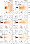 |
Fig. 7 Plasma stream propagating through the zero magnetic field region for different target positions. Interferometry measurements are at 68 ns after laser irradiation of the target. The gray rectangle indicates the location of the target. To depict the position of the target and reduce the scale of the picture, panels c–f are drawn with a gap, represented by the dashed line. |
4 Scalability to astrophysical plasmas
4.1 Jet parameters
The plasma density and temperature, as well as the strength of the poloidal magnetic field, vary greatly from the jet source region to its head. Regardless of the source of the winds (stellar or disk), the outflows are initially magnetically dominated.
Further, the flows are accelerated, magneto-centrifugally for the case of disk winds (Blandford & Payne 1982; Ferreira 1997) and by Alfvén waves or pressure gradients in the stellar corona for the stellar winds (Suzuki & Inutsuka 2006; Cranmer et al. 2007). During acceleration, the outflow’s ram pressure increases and becomes equal to the magnetic pressure on the Alfvén surface where the wind velocity reaches the Alfvén velocity  . It is believed that diverging winds start collimating beyond the Alfvén surface (Pelletier & Pudritz 1992) and it is this region with ram pressure-dominated plasma flow that is favorably reproduced in our laboratory experiment. Since our study is focused mainly on the issues of jet collimation by large-scale divergent poloidal magnetic fields, we consider regions tens AU away from the Alfvén surface to construct a scaling between the astrophysical and laboratory jets. A typical magnetic field in this region varies from 0.03 to 0.08 G; a typical outflow density ne varies from 4 × 10⁴ to 106 cm−3 (Hartigan et al. 2007; Coffey et al. 2008).
The typical value for the plasma temperature in the collimation region is assumed to be 20–50 kK (Coffey et al. 2008; Schneider et al. 2013). Since the flow velocity varies weakly throughout the entire jet, a realistic value to be taken into account for the YSO jets is 250 km s−1 (Hartigan et al. 2007; Schneider et al. 2013). Referring to the same authors, we assume that the characteristic scale L (width) of the jet near the source is about 30 AU. The corresponding scale L in laboratory experiments, as can be seen in Figs. 7 and 5, is about 1 cm.
4.2 Scalability of laboratory plasma to YSOs
The scalability of the laboratory plasma stream to the astrophysical jet of the YSOs is based on Ryutov’s Euler similarity approach, which is described in detail in (Ryutov et al. 1999, 2000; Ryutov 2018). The scaling of two systems is possible if the two parameters are similar, the Euler number (Eu = V(ρ/p)1/2) and the plasma beta (β = 8πp/B2), where V is the flow velocity, ρ is the mass density, p = kB(niTi + neTe) is the thermal pressure (kB is the Boltzmann constant, ni,e and Ti,e are the number densities and temperatures of the ions and electrons, respectively), and B is the magnetic field. In this case scaled systems evolve in the same way.
The Euler similarity is derived within the framework of ideal MHD equations, which is when dissipative processes can be neglected. Therefore, three parameters, namely the Reynolds number, the magnetic Reynolds number, and the Peclet number, should be higher than 1. The first parameter is the Reynolds number, Re = LV/v, which is responsible for the viscous dissipation, where L is the characteristic spatial scale, V is the flow velocity, and
![Mathematical equation: $v\left[ {{\rm{c}}{{\rm{m}}^2}{{\rm{s}}^{ - 1}}} \right] = 1.4 \times {10^9}{{{T_i}{{[{\rm{kK}}]}^{2.5}}} \over {{\rm{\Lambda }}\sqrt A {Z^4}{n_i}}}$](/articles/aa/full_html/2024/01/aa45251-22/aa45251-22-eq3.png) (1)
(1)
is the kinematic viscosity (Ryutov et al. 1999, p. 825) with Λ the Coulomb logarithm and A the averaged atomic weight. The second parameter is the magnetic Reynolds number, ReM = LV/η, which is responsible for the resistive diffusion, where
 (2)
(2)
is the magnetic diffusivity (Ryutov et al. 2000), σ is the electrical conductivity, me is the electron mass, and e is the electron charge. Finally, the third parameter is the Peclet number, Pe = LV/χ, which is responsible for the thermal conduction, the ratio of heat convection to the heat conduction, where
![Mathematical equation: $\chi \left[ {{\rm{c}}{{\rm{m}}^2}{{\rm{s}}^{ - 1}}} \right] = 1.4 \times {10^{11}}{{{T_i}{{[kK]}^{2.5}}} \over {{\rm{\Lambda }}Z(Z + 1){n_i}}}$](/articles/aa/full_html/2024/01/aa45251-22/aa45251-22-eq5.png) (3)
(3)
is the thermal diffusivity (Ryutov et al. 1999, p. 824).
We verified (see Table 1) that these three parameters are higher than unity for both the YSO and laboratory plasmas, which supports the validity of the Euler similarity. Moreover, we show that the Euler number and plasma-β values are well matched between the laboratory and the YSO jets, confirming the similarity of the evolution of the considered plasma outflows and jets.
Table 1 also summarizes other important parameters of the laboratory plasma flow, as well as of YSOs outflows, such as the deceleration radius Rb, which determines the radial scale of the plasma cavity. The simplest estimate for Rb can be derived in spherical symmetry by considering when the magnetic pressure is in equilibrium with the plasma ram pressure. This estimate indicates that for a reasonable magnetic field and mass outflow rate the collimation can be achieved over length scales consistent with observation and numerical models (Günther et al. 2014; Ustamujic et al. 2018). The estimate of Rb for YSO in Table 1 was done assuming a quasi-uniform magnetic field using formula in CGS units  (Matt et al. 2003; Günther et al. 2014) (we take Ṁ = 10−8M⊙ yr−1, Coffey et al. 2008).
We can estimate the magnetic flux requarements of the astrophysical jet for effective collimation (following the work of Cabrit 2007) as Ψ ~ π  Bz ≈ 4×1027 G cm2, where rmax is the scale of the annular region over which the magnetic field needs to be anchored to the disk and is fairly well estimated by the value of Rb ~ 1.6 × 1014 cm. The value of the corresponding magnetic flux Ψ is 0.1 % of the flux present before gravitational collapse (ΨB)crit ≈ 4 × 1030(M/1M⊙) G cm2 (Cabrit 2007; Mouschovias & Spitzer Jr 1976), which correlates very well with the relation in magnetic flux values that are reserved for launching of magnetically driven GRB jets (Komissarov & Barkov 2009; Barkov & Komissarov 2010).
Under more realistic conditions the magnetic field is expected to be nonuniform and to decrease with distance from the outflow axis and from the source. Modern observations resolve the structure of magnetic fields for Class 0, I protostars only at scales of 300 AU or more (Girart et al. 2006; Kwon et al. 2019; Hull et al. 2020). In particular, on large scales (up to 1000–2000 AU) the poloidal magnetic field can be approximated as a radial split-monopole field (B ~ r−2, Galli & Shu 1993a,b; Galli et al. 2006). The field structure on smaller scales (10–100 AU) has been reconstructed using numerical and analytical calculations, while comparing asymptotic behavior with observations (Gonçalves et al. 2008). The accuracy of such a reconstruction is not high and still requires further investigations.
There are no detailed calculations for the recollimation length 2Rb in the nonuniform case, but the simplest idea (Matt et al. 2003; Kwan & Tademaru 1995) is that as the wind expands its ram pressure decreases with radius as Pram = ρV2 ~ r−2, and assuming the magnetic field decrease as B ~ r−n, the magnetic pressure behaves as Pmag ~ r−2n. Thus, it seems that for n > 1 the magnetic pressure decreases too quickly and the balance is not achievable, hence no cavity is formed and recollimation does not occur. On the contrary, since the plasma is highly conductive and its expansion is super magnetosonic, it is able to sweep up and compress the magnetic field, forming shocks on the boundary; the modeling of this process can be seen in the recent MHD simulation (Jannaud et al. 2023). Furthermore, the magnetic field lines are also anchored in the disk, and magnetic tensions in addition to pressure also play an important role. Hence, the question of whether a cavity with a magnetic nozzle could be formed in such a diverging magnetic field requires a more comprehensive analysis. We plan to study this in our future work.
Comparison and scalability between the laser-driven plasma stream and a YSO jet.
5 Three-dimensional numerical modeling
To complement the previous analysis, in this section we present end-to-end full-scale numerical simulations using the hybrid approach. While we do not aim to perform a one-to-one simulation of the experiment, due to a restriction of computational resources, by modeling a pure hydrogen plasma we are able to reproduce the experimental aspect ratio of the jet and plasma temperature features.
To properly describe the interaction of ions with the magnetic field, we use the Arbitrary Kinetic Algorithm (AKA) hybrid code (Sladkov 2023), built on general and well-assessed principles of previous codes (Winske et al. 2003), such as Heckle (Smets et al. 2011), with advanced features, for example an ablation operator and a six-component electron pressure tensor. In the numerical model, the ion description follows the Particle-In-Cell formalism, and the electrons are described by the ten-moment model. These ten moments are density (n, equal to the total ion density by quasi-neutrality), bulk velocity (Ve), and the six-component electron pressure tensor (Pe). The electromagnetic fields are treated in the low-frequency (Darwin) approximation, neglecting the displacement current. The generalized Ohm’s law contains three terms: (i) Vi × B, where Vi is the ion bulk velocity; (ii) (J × B)/en, the Hall effect, which describes the ions decoupling from the magnetic field, where J is the total current density and is equal to the curl of B; and (iii) (∇ ⋅ Pe)/en, the divergence of the electron pressure tensor, which represents the electron fluid contribution (Sladkov et al. 2021). Ion-ion collisions were taken into account using the Takizuka-Abe binary collision model (Takizuka & Abe 1977).
In the model the magnetic field and density are normalized to B0 = 5 × 10⁵ G and n0 = 2 × 1020 cm−3, respectively, and the normalization of the other quantities follows from them. The density defines the inertial length of the ion, d0 ~ 16 µm, which determines the length normalization. The box is 3D rectangular (200 × 200 × 500d0 in size), and the maximum height of the jet is 8 mm in this normalization. The magnetic field defines the temporal normalization since the time is normalized to the inverse of the ion gyrofrequency,  , which is ~0.2 ns. The velocities are normalized to the Alfvén velocity V0 (calculated using B0 and n0), which is 77 km s−1. In the simulation, the target density was initialized to 5n0 (i.e., 1021 cm−3), and the magnetic field (along the z-axis), to 0.2B0 (i.e., 105 G).
Continuous plasma production by the laser-target interaction is imitated by the ablation operator (Sladkov et al. 2020), which is responsible for the heating of ions and electrons and the creation of ions. The particle creation operator allows a constant target density, mimicking the reservoir of a solid-density target. The heat operator pumps the electron pressure linearly into the near target-surface region, creating a pressure gradient along the normal to the target surface; this generates an electric field and accelerates ions, triggering the plasma expansion. The magnitude of the heat operator is adjusted to obtain the desired temperature for both ions and electrons ( , which is 730 kK for the chosen parameters). The ablation operator is turned on for tΩ0 < 12.5, after which the pressure pumping is turned off and the particles are loaded with cold temperature, the diameter of the heated area is 30d0.
Figure 8 illustrates the evolution of the plasma plume in the uniform external magnetic field. At first, once the cavity is formed (tΩ0 = 75), on the top of the cavity (150d0 < z < 180d0) we observe that the magnetic field is compressed and grows five times stronger (Fig. 8c), which is attributed to the conical shock (Revet et al. 2021). Panel d displays the analog of the interferom-etry at the end of the simulation (tΩ0 = 125). Compared with the experimental figures (Fig. 5), we see a good agreement, even if the experimental interferometry resolves only one order of magnitude. The flow velocity in the axial direction is ~4V0, which corresponds to ~300 km s−1. Plotting the ram pressure of the ions (Fig. 8c) at tΩ0 = 100, we can find the flow driver (340d0 < z < 380d0). As pointed out previously (Higginson et al. 2017), this part is marginally magnetized and maintains a high aspect ratio due to its high Mach number.
In Fig. 8, panels e, f, and g display the parallel ion temperature, perpendicular ion temperature, and the electron temperature, respectively, as color-coded images. Each panel represents a two-dimensional generalization of a lineout, where the abscissa axis represents time and the ordinate axis represents the Z coordinate. These panels capture the time evolution of a vertical lineout along the central axis of the jet. Panels e and f reveal that the ion temperature remains relatively uniform within the interior of the jet. This uniformity is primarily due to efficient ion-ion collision processes that equilibrate the ion temperatures. The perpendicular ion temperature (panel f) remains around the initial focal spot temperature 1T0. The electron temperature distribution along the central axis of the jet (panel g) suggests that the electron heating is predominantly confined by the compressed magnetic field; the estimated deceleration radius is approximately 150d0 (i.e., 2.4 mm). Using these parameters, the Mach number (the ratio of the ion flow velocity to the ion sound speed) is around 5, which can approach the value estimated experimentally (~ 10) by using heavy ions with a realistic charge-to-mass ratio (1/10) and the same flow velocity distribution.
To reproduce the experiments with the diverging magnetic field and to support the hypothesis of the possibility to maintain a narrow jet even in the space without an ambient magnetic field, we also simulated the evolution of a plasma plume in a nonuniform magnetic field modeling the experimental magnet, but we put the magnetic field strength in the region z > 0 (i.e., beyond the magnetic field reversal point) to zero. We expect that the stopping radius in the axial direction should be about 150d0, and we model two configurations with long (360d0, Figs. 9a– d) and short (180d0, Figs. 9e–h) gradients of the magnetic field pressure. In both cases the gradient length is enough for the conical shock to form (Albertazzi et al. 2014; Higginson et al. 2017) (Figs. 9b, f), which redirects the flow into a jet. The short gradient case shows a jet that is less collimated than in the uniform case. There the cavity finishes its formation in the volume that is free from the high magnetic pressure, which does not allow the jet to be recollimated into a narrow structure after flowing around the top conical shock. As a result, above the conical shock we see a diverging tip of the jet (Fig. 9h). This case can be found in the experimental data (Figs. 7b, c). Looking at the long-gradient case (Figs. 9a–d), we observe a well-collimated plasma jet, which is narrow enough to be comparable with the laboratory observations, see Figs. 7d, f.
In conclusion, the collimation of plasma outflows into narrow jets is possible through the interaction of initially diverging plasma flows with strong poloidal magnetic field region. The numerical results suggest that this interaction can lead to the formation of a plasma cavity with a compressed magnetic field region which redirects the plasma flow into a tightly focused jet. Future numerical investigations are needed to explore the underlying mechanisms responsible for the formation and stability of the real astrophysical jets, taking into account such effects as gravitation and the associated rotation of the object.
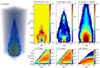 |
Fig. 8 Results of the three-dimensional hybrid simulation by the AKA code conducted in a uniform external magnetic field. Panel a: snapshot of the plasma density surrounded by the magnetic pressure. Panels b, c: plasma parameters in the median plane. Panel d: integrated plasma density along the x-axis. Panels e–g: evolution of the central axial lineout for the plasma temperature: (e) ion temperature parallel to magnetic field; (f) perpendicular ion temperature; (g) electron temperature, defined as one-third of the electron pressure tensor divided by density. The temporal and spatial normalization factors are, respectively, |

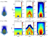 |
Fig. 9 Results of the three-dimensional hybrid simulation by the AKA code for two different diverging magnetic field configurations (top and bottom). Panels a, e: snapshot of the plasma density surrounded by the magnetic pressure. Panels b, c, f, g: magnetic pressure in the median plane. Panels d, h: integrated plasma density along the x-axis. The temporal and spatial normalization factors are, respectively, |

6 Summary
The exact mechanism of jet collimations is still under debate. Laboratory studies, such as the one presented here, are of particular importance as they allow us to address extreme flow conditions that are only accessible to simulations, and thus can help validate these models.
In the present study we conducted scaled laboratory experiments at the PEARL laser facility to explore the role of a poloidal magnetic field on the confinement of a wide angle flow and the formation of a jet. Unlike previous experimental works (Albertazzi et al. 2014; Higginson et al. 2017) and simulations (Matt et al. 2003; Ciardi et al. 2013; Ustamujic et al. 2018), we explored the impact of a diverging magnetic field on the flow dynamics.
We observed that a strong poloidal magnetic field region can lead to the generation of a plasma cavity with a magnetic nozzle tip and, as a result, it can collimate the outflow into a narrow jet. We studied experimentally and numerically how the collimation process depends on the scale of a region where a strong poloidal magnetic field is present, and found that the minimum scale-length of this region has to be on the order of 2Rb to collimate the flow. We also investigated the propagation of the plasma flow through the region with highly diverging magnetic field lines and zero point. In particular, we observed that the propagation of the jet proceeds unimpeded and maintains a high aspect ratio. This indicates that once the jet is formed, it propagates balistically and that its bulk kinetic energy dominates the magnetic field energy. The dynamics of the plasma is well recovered by kinetic hybrid-PIC simulations, including the effect of a rapidly decreasing magnetic field.
As was shown in Sect. 4.2, the scaling of the astrophysical and laboratory systems works with reasonable accuracy, indicating that our experimental approach could be used to interpret the structure and morphology of protostellar jets collimated in a large-scale divergent poloidal magnetic field. The exact structure of the magnetic field near a YSO (at scales of tens of AU) has not yet been determined, so it is speculative to compare it with the topology of the magnetic field reproduced in the experiment. However, in our experimental model the fundamental requirements for the divergence of magnetic fields that are able to affect collimation have been demonstrated. Some conditions still need to be verified numerically, but our laboratory model can already help in understanding the mechanisms of jet collimation. Finally, we emphasize that the collimation discussed in this work is not in contradiction with models of self-collimation by a toroidal magnetic field (Blandford & Payne 1982; Ferreira 1997), but it can be complementary, as in the work of Matsakos et al. (2009), who studied numerically the interaction of a stellar wind with a disk wind.
Acknowledgements
This work was supported by the European Research Council (ERC) under the European Union’s Horizon 2020 research and innovation program (Grant Agreement No. 787539). The experiments at the PEARL laser facility were supported by 10th project of the National Center for Physics and Mathematics (NCPhM) “Experimental laboratory astrophysics and geophysics”. A.Z. was supported by the Russian Foundation for Basic Research, project no. 19-29-11013. R.Z., K.B., A.S., A.K., M.S., S.P. acknowledge support from the Ministry of Higher Education and Science of the Russian Federation (project no. 075-15-2021-1361). The simulations were performed on resources provided by the Joint Supercomputer Center of the Russian Academy of Sciences.
References
- Albertazzi, B., Ciardi, A., Nakatsutsumi, M., et al. 2014, Science, 346, 325 [NASA ADS] [CrossRef] [Google Scholar]
- Allen, A., Shu, F. H., & Li, Z.-Y. 2003, ApJ, 599, 351 [NASA ADS] [CrossRef] [Google Scholar]
- Anathpindika, S., & Whitworth, A. P. 2008, A&A, 487, 605 [NASA ADS] [CrossRef] [EDP Sciences] [Google Scholar]
- Anglada, G., Rodríguez, L. F., & Carrasco-González, C. 2018, A&ARv, 26, 1 [NASA ADS] [CrossRef] [Google Scholar]
- Bally, J., Reipurth, B., & Davis, C. J. 2007, Protostars and Planets V, 215 [Google Scholar]
- Barkov, M. V., & Komissarov, S. S. 2010, MNRAS, 401, 1644 [NASA ADS] [CrossRef] [Google Scholar]
- Begelman, M. C. 1998, ApJ, 493, 291 [NASA ADS] [CrossRef] [Google Scholar]
- Bellan, P. 2018, J. Plasma Phys., 84 [CrossRef] [Google Scholar]
- Blandford, R. D., & Payne, D. G. 1982, MNRAS, 199, 883 [CrossRef] [Google Scholar]
- Burdonov, K., Bonito, R., Giannini, T., et al. 2021, A&A, 648, A81 [NASA ADS] [CrossRef] [EDP Sciences] [Google Scholar]
- Burdonov, K., Yao, W., Sladkov, A., et al. 2022, A&A, 657, A112 [NASA ADS] [CrossRef] [EDP Sciences] [Google Scholar]
- Cabrit, S. 2007, Proc. Int. Astron. Union, 3, 203 [NASA ADS] [CrossRef] [Google Scholar]
- Ciardi, A., Lebedev, S., Frank, A., et al. 2007, Phys. Plasmas, 14, 056501 [Google Scholar]
- Ciardi, A., Vinci, T., Fuchs, J., et al. 2013, Phys. Rev. Lett., 110, 025002 [Google Scholar]
- Coffey, D., Bacciotti, F., & Podio, L. 2008, ApJ, 689, 1112 [NASA ADS] [CrossRef] [Google Scholar]
- Cranmer, S. R., Van Ballegooijen, A. A., & Edgar, R. J. 2007, ApJS, 171, 520 [NASA ADS] [CrossRef] [Google Scholar]
- Dupree, A., Brickhouse, N., Smith, G. H., & Strader, J. 2005, ApJ, 625, L131 [CrossRef] [Google Scholar]
- Edwards, S., Fischer, W., Kwan, J., Hillenbrand, L., & Dupree, A. K. 2003, ApJ, 599, L41 [NASA ADS] [CrossRef] [Google Scholar]
- Edwards, S., Fischer, W., Hillenbrand, L., & Kwan, J. 2006, ApJ, 646, 319 [Google Scholar]
- Faenov, A. Y., Pikuz, S., Erko, A., et al. 1994, Physica Scripta, 50, 333 [NASA ADS] [CrossRef] [Google Scholar]
- Ferreira, J. 1997, A&A, 319, 340 [Google Scholar]
- Ferreira, J., Pelletier, G., & Appl, S. 2002, MNRAS, 312, 387 [Google Scholar]
- Ferreira, J., Dougados, C., & Cabrit, S. 2006, A&A, 453 [Google Scholar]
- Galli, D., & Shu, F. H. 1993a, ApJ, 417, 220 [NASA ADS] [CrossRef] [Google Scholar]
- Galli, D., & Shu, F. H. 1993b, ApJ, 417, 243 [NASA ADS] [CrossRef] [Google Scholar]
- Galli, D., Lizano, S., Shu, F. H., & Allen, A. 2006, ApJ, 647, 374 [NASA ADS] [CrossRef] [Google Scholar]
- Ginzburg, V., Yakovlev, I., Kochetkov, A., et al. 2021, Opt. Exp., 29, 28297 [CrossRef] [Google Scholar]
- Girart, J. M., Crutcher, R. M., & Rao, R. 1999, ApJ, 525, L109 [NASA ADS] [CrossRef] [Google Scholar]
- Girart, J. M., Rao, R., & Marrone, D. P. 2006, Science, 313, 812 [Google Scholar]
- Günther, H. M., Li, Z.-Y., & Schneider, P. C. 2014, ApJ, 795, 51 [CrossRef] [Google Scholar]
- Gonçalves, J., Galli, D., & Girart, J. M. 2008, A&A, 490, L39 [NASA ADS] [CrossRef] [EDP Sciences] [Google Scholar]
- Goodson, A. P., Böhm, K.-H., & Winglee, R. M. 1999, ApJ, 524, 142 [NASA ADS] [CrossRef] [Google Scholar]
- Hartigan, P., Frank, A., Varniere, P., & Blackman, E. 2007, ApJ, 661, 910 [NASA ADS] [CrossRef] [Google Scholar]
- Higginson, D., Revet, G., Khiar, B., et al. 2017, High Energy Density Physics, 23 [Google Scholar]
- Hull, C. L., Le Gouellec, V. J., Girart, J. M., Tobin, J. J., & Bourke, T. L. 2020, ApJ, 892, 152 [NASA ADS] [CrossRef] [Google Scholar]
- Jacquemin-Ide, J., Lesur, G., & Ferreira, J. 2021, A&A, 647, A192 [EDP Sciences] [Google Scholar]
- Jannaud, T., Zanni, C., & Ferreira, J. 2023, A&A, 669, A159 [NASA ADS] [CrossRef] [EDP Sciences] [Google Scholar]
- Kamali, F., Henkel, C., Koyama, S., et al. 2019, A&A, 624, A42 [NASA ADS] [CrossRef] [EDP Sciences] [Google Scholar]
- Komissarov, S. S., & Barkov, M. V. 2009, MNRAS, 397, 1153 [NASA ADS] [CrossRef] [Google Scholar]
- Königl, A., & Salmeron, R. 2010, Physical Processes in Circumstellar Disks around Young Stars, ed. P. J. V. Garcia (Chicago, IL: University of Chicago Press), 283 [Google Scholar]
- Korobkov, S., Nikolenko, A., Gushchin, M., et al. 2023, Astron. Rep., 67, 93 [NASA ADS] [CrossRef] [Google Scholar]
- Kwan, J., & Tademaru, E. 1995, ApJ, 454, 382 [NASA ADS] [CrossRef] [Google Scholar]
- Kwan, J., Edwards, S., & Fischer, W. 2007, ApJ, 657, 897 [Google Scholar]
- Kwon, W., Stephens, I. W., Tobin, J. J., et al. 2019, ApJ, 879, 25 [NASA ADS] [CrossRef] [Google Scholar]
- Lai, S.-P., Crutcher, R. M., Girart, J. M., & Rao, R. 2002, ApJ, 566, 925 [NASA ADS] [CrossRef] [Google Scholar]
- Li, J., & Cao, X. 2019, ApJ, 872, 149 [NASA ADS] [CrossRef] [Google Scholar]
- Lozhkarev, V. V., Freidman, G. I., Ginzburg, V. N., et al. 2007, Laser Phys. Lett., 4, 421 [Google Scholar]
- Luchinin, A., Malyshev, V., Kopelovich, E., et al. 2021, Rev. Sci. Instrum., 92, 123506 [NASA ADS] [CrossRef] [Google Scholar]
- Matsakos, T., Massaglia, S., Trussoni, E., et al. 2009, A&A, 502, 217 [NASA ADS] [CrossRef] [EDP Sciences] [Google Scholar]
- Matt, S., & Pudritz, R. 2005, ApJ, 632 [Google Scholar]
- Matt, S., & Pudritz, R. E. 2008, ApJ, 678, 1109 [NASA ADS] [CrossRef] [Google Scholar]
- Matt, S., Winglee, R., & Böhm, K.-H. 2003, MNRAS, 345, 660 [NASA ADS] [CrossRef] [Google Scholar]
- Moll, R. 2009, A&A, 507, 1203 [NASA ADS] [CrossRef] [EDP Sciences] [Google Scholar]
- Moll, R., Spruit, H., & Obergaulinger, M. 2008, A&A, 492, 621 [NASA ADS] [CrossRef] [EDP Sciences] [Google Scholar]
- Mouschovias, T. C., & Spitzer Jr, L. 1976, ApJ, 210, 326 [NASA ADS] [CrossRef] [Google Scholar]
- Pelletier, G., & Pudritz, R. E. 1992, ApJ, 394, 117 [NASA ADS] [CrossRef] [Google Scholar]
- Pudritz, R. E., Ouyed, R., & Brandenburg, A. 2007, Protostars and planets V, 277 [Google Scholar]
- Ray, T., Poetzel, R., Solf, J., & Mundt, R. 1990, ApJ, 357, L45 [NASA ADS] [CrossRef] [Google Scholar]
- Revet, G. 2018, Theses, Université Paris Saclay (COmUE) [Google Scholar]
- Revet, G., Khiar, B., Filippov, E., et al. 2021, Nat. Commun., 12, 1 [CrossRef] [Google Scholar]
- Ryutov, D. D. 2018, Phys. Plasmas, 25, 100501 [Google Scholar]
- Ryutov, D., Drake, R. P., Kane, J., et al. 1999, A&A, 518, 821 [Google Scholar]
- Ryutov, D. D., Drake, R. P., & Remington, B. A. 2000, ApJS, 127, 465 [Google Scholar]
- Schleuning, D. 1998, ApJ, 493, 811 [NASA ADS] [CrossRef] [Google Scholar]
- Schneider, P., Eislöffel, J., Güdel, M., et al. 2013, A&A, 550, A1 [Google Scholar]
- Shu, F., Najita, J., Ostriker, E., et al. 1994, ApJ, 429, 781 [Google Scholar]
- Sladkov, A. 2023, https://doi.org/10.5281/zenodo.7878463 [Google Scholar]
- Sladkov, A., Smets, R., & Korzhimanov, A. 2020, J. Phys. Conf. Ser., 1640, 012011 [NASA ADS] [CrossRef] [Google Scholar]
- Sladkov, A., Smets, R., Aunai, N., & Korzhimanov, A. 2021, Phys. Plasmas, 28, 072108 [NASA ADS] [CrossRef] [Google Scholar]
- Smets, R., Belmont, G., Aunai, N., & Rezeau, L. 2011, Phys. Plasmas, 18 [CrossRef] [Google Scholar]
- Soloviev, A., Burdonov, K., Kotov, A., et al. 2021, Radiophys. Quant. Electron., 63, 876 [NASA ADS] [CrossRef] [Google Scholar]
- Soloviev, A., Kotov, A., Martyanov, M., et al. 2022, Opt. Express, 30, 40584 [CrossRef] [Google Scholar]
- Spruit, H., Foglizzo, T., & Stehle, R. 1997, MNRAS, 288, 333 [NASA ADS] [CrossRef] [Google Scholar]
- Suzuki, T. K., & Inutsuka, S.-i. 2006, J. Geophys. Res. Space Phys., 111 [Google Scholar]
- Takizuka, T., & Abe, H. 1977, J. Comput. Phys., 25, 205 [CrossRef] [Google Scholar]
- Ustamujic, S., Orlando, S., Bonito, R., Miceli, M., & Gómez de Castro, A. 2018, A&A, 615 [NASA ADS] [CrossRef] [EDP Sciences] [Google Scholar]
- Winske, D., Yin, L., Omidi, N., Karimabadi, H., & Quest, K. 2003, Hybrid Simulation Codes: Past, Present and Future – A Tutorial, eds. J. Büchner, M. Scholer, & C. T. Dum (Berlin, Heidelberg: Springer Berlin Heidelberg), 136 [Google Scholar]
- Winske, D., Huba, J., Niemann, C., & Le, A. 2019, Front. Astron. Space Sci., 5, 51 [NASA ADS] [CrossRef] [Google Scholar]
- Wright, G. 1973, MNRAS, 162, 339 [NASA ADS] [CrossRef] [Google Scholar]
- Zakharov, Y., Antonov, V., Boyarintsev, E., et al. 2006, Plasma Phys. Rep., 32, 183 [NASA ADS] [CrossRef] [Google Scholar]
- Zhu, Z., & Stone, J. 2017, ApJ, 857, 34 [Google Scholar]
All Tables
All Figures
|
Fig. 1 Modeling setup. Left: schematic representation of the large-scale structure of the interstellar magnetic field disturbed by the accretion disk of a young stellar object (YSO) and taking the shape of an hourglass. The structure of the magnetic fields in the figure is an example and not a complete match. The red arrows indicate axisymmetric jets. The blue rectangle shows the area modeled in the experiment. Right: schematic of the experiment indicating the magnetic field structure with a plasma outflow. The shaded areas are unavailable for diagnostics; the white area illustrates the diagnostic window. |
| In the text | |
|
Fig. 2 Schematic view of the experimental setup. 1 – Nanosecond heating laser pulse, 2 – Femtosecond laser probe pulse, 3 – Windings, 4 – Teflon target. |
| In the text | |
|
Fig. 3 Schematic sectional view of our magnetic system (a), the 3D model of the load-bearing metal frame (b), and a photo of the manufactured magnetic system (c). The numbers indicate the following: 1 - Load-bearing metal frame, 2 – Composite elements of the load-bearing frame, 3 – Windings, 4 – Nitrogen chamber, 5 – External shield, 6 – Conical holes for laser radiation input and plasma flow output, 7 – Channels for liquid nitrogen supply and placement of current leads, and 8 – Vacuum-tight bellows docking unit. The figure is from the article Luchinin et al. (2021), which presents the development of the magnetic system. |
| In the text | |
|
Fig. 4 Structure of the magnetic field: (a) co-directional connection of the coils, (b) oppositely directed connection, (c) Bz profiles on the axis of the magnetic system. |
| In the text | |
|
Fig. 5 Two-dimensional density profiles of the plasma stream propagating along a quasi-uniform magnetic field at 28 ns (a), 38 ns (b), 48 ns (c), and 68 ns (d) after the laser irradiation of the target. The spatial scale shown in (a) is the same for all the images. To demonstrate the evolution of the plasma cavity, the position of the target was shifted from shot to shot. Each panel in this figure is composed of a few such experimental snapshots. |
| In the text | |
|
Fig. 6 Two-dimensional density profiles of the plasma stream propagating through a poloidal diverging magnetic field at 28 ns (a, b) and 48 ns (c, d) after laser irradiation of the target. The gray rectangle shows the location of the target. To depict the position of the target and reduce the scale of the picture, panel d is drawn with a gap, represented by the dashed line. |
| In the text | |
|
Fig. 7 Plasma stream propagating through the zero magnetic field region for different target positions. Interferometry measurements are at 68 ns after laser irradiation of the target. The gray rectangle indicates the location of the target. To depict the position of the target and reduce the scale of the picture, panels c–f are drawn with a gap, represented by the dashed line. |
| In the text | |
|
Fig. 8 Results of the three-dimensional hybrid simulation by the AKA code conducted in a uniform external magnetic field. Panel a: snapshot of the plasma density surrounded by the magnetic pressure. Panels b, c: plasma parameters in the median plane. Panel d: integrated plasma density along the x-axis. Panels e–g: evolution of the central axial lineout for the plasma temperature: (e) ion temperature parallel to magnetic field; (f) perpendicular ion temperature; (g) electron temperature, defined as one-third of the electron pressure tensor divided by density. The temporal and spatial normalization factors are, respectively, |
| In the text | |
|
Fig. 9 Results of the three-dimensional hybrid simulation by the AKA code for two different diverging magnetic field configurations (top and bottom). Panels a, e: snapshot of the plasma density surrounded by the magnetic pressure. Panels b, c, f, g: magnetic pressure in the median plane. Panels d, h: integrated plasma density along the x-axis. The temporal and spatial normalization factors are, respectively, |
| In the text | |
Current usage metrics show cumulative count of Article Views (full-text article views including HTML views, PDF and ePub downloads, according to the available data) and Abstracts Views on Vision4Press platform.
Data correspond to usage on the plateform after 2015. The current usage metrics is available 48-96 hours after online publication and is updated daily on week days.
Initial download of the metrics may take a while.