| Issue |
A&A
Volume 667, November 2022
|
|
|---|---|---|
| Article Number | A127 | |
| Number of page(s) | 9 | |
| Section | Planets and planetary systems | |
| DOI | https://doi.org/10.1051/0004-6361/202244280 | |
| Published online | 18 November 2022 | |
Planet-star interactions with precise transit timing
III. Entering the regime of dynamical tides★,★★
1
Institute of Astronomy, Faculty of Physics, Astronomy and Informatics, Nicolaus Copernicus University in Toruń,
Grudziadzka 5,
87-100
Toruń, Poland
e-mail: gmac@umk.pl
2
Instituto de Astrofísica de Andalucía (IAA-CSIC),
Glorieta de la Astronomía 3,
18008
Granada, Spain
3
Institute of Astronomy and National Astronomical Observatory, Bulgarian Academy of Sciences,
72 Tsarigradsko Chaussee Blvd.,
1784
Sofia, Bulgaria
4
Michael Adrian Observatorium, Astronomie Stiftung Trebur,
65428
Trebur, Germany
5
University of Applied Sciences, Technische Hochschule Mittelhessen,
61169
Friedberg, Germany
6
Astrophysikalisches Institut und Universitäts-Sternwarte,
Schillergässchen 2,
07745
Jena, Germany
7
Valencia International University,
46002
Valencia, Spain
Received:
15
June
2022
Accepted:
21
September
2022
Context. Hot Jupiters on extremely short-period orbits are expected to be unstable due to tidal dissipation and spiral toward their host stars. That is because they transfer the angular momentum of the orbital motion through tidal dissipation into the stellar interior. Although the magnitude of this phenomenon is related to the physical properties of a specific star-planet system, statistical studies show that tidal dissipation might shape the architecture of hot Jupiter systems during the stellar lifetime on the main sequence.
Aims. The efficiency of tidal dissipation remains poorly constrained in star-planet systems. Stellar interior models show that the dissipation of dynamical tides in radiation zones could be the dominant mechanism driving planetary orbital decay. These theoretical predictions can be verified with the transit timing method.
Methods. We acquired new precise transit mid-times for five planets. They were previously identified as the best candidates for which orbital decay might be detected. Analysis of the timing data allowed us to place tighter constraints on the orbital decay rate.
Results. No statistically significant changes in their orbital periods were detected for all five hot Jupiters in systems HAT-P-23, KELT-1, KELT-16, WASP-18, and WASP-103. For planets HAT-P-23 b, WASP-18 b, and WASP-103 b, observations show that the mechanism of the dynamical tidal dissipation probably does not operate in their host stars, preventing their orbits from rapidly decaying. This finding aligns with the models of stellar interiors of F-type stars, in which dynamical tides are not fully damped due to convective cores. For KELT-16 b, the span of transit timing data was not long enough to verify the theoretical predictions. KELT-1 b was identified as a potential laboratory for studying the dissipative tidal interactions of inertial waves in a convective layer. Continued observations of those two planets may provide further empirical verification of the tidal dissipation theory.
Key words: planet-star interactions / planets and satellites: dynamical evolution and stability / methods: observational / techniques: photometric
The ground-based light curves and the full Table A.2 are only available at the CDS via anonymous ftp to cdsarc.cds.unistra.fr (130.79.128.5) or via https://cdsarc.cds.unistra.fr/viz-bin/cat/J/A+A/667/A127
This research is partly based on: (1) data obtained at the 1.5 m telescope of the Sierra Nevada Observatory (Spain), which is operated by the Consejo Superior de Investigaciones Científicas (CSIC) through the Instituto de Astrofísica de Andalucía; (2) observations collected with telescopes at the Rozhen National Astronomical Observatory; and (3) observations obtained with telescopes of the University Observatory Jena, which is operated by the Astrophysical Institute of the Friedrich-Schiller-University.
© G. Maciejewski et al. 2022
 Open Access article, published by EDP Sciences, under the terms of the Creative Commons Attribution License (https://creativecommons.org/licenses/by/4.0), which permits unrestricted use, distribution, and reproduction in any medium, provided the original work is properly cited.
This article is published in open access under the Subscribe-to-Open model. Subscribe to A&A to support open access publication.
1 Introduction
The statistical studies of the planetary systems harbouring hot Jupiters provide substantial evidence of dissipative tidal interactions between those massive planets and their host stars. In a typical configuration, in which the host star rotates slower than its close planetary companion orbits it, the angular momentum of the orbital motion is transferred into the stellar spin due to tidal dissipation in the stellar interior. The population of hot Jupiter host stars was found to have a lower Galactic velocity dispersion than the field stars in a reference sample (Hamer & Schlaufman 2019). This kinematical youth suggests that their planets must spiral in due to tidal interactions in timescales noticeably shorter than the stellar evolution on the main sequence. Furthermore, the host stars with close-orbiting giant planets tend to be younger in gyro-chronological dating compared to their ages determined from stellar-evolutionary models (Brown 2014; Maxted et al. 2015; Tejada Arevalo et al. 2021). They are supposed to rotate faster because their spiralling-in planets have spun them up.
The magnitude of tidal dissipation in a star is quantified by a modified tidal quality factor, defined as
 (1)
(1)
where Etide is the maximum energy stored in the tide, D is the dissipation integrated over the tidal period Ptide, and k2 is the second-order potential Love number (Barker 2020). The tidal period is related to the stellar rotation period P* and the planetary orbital period Porb with the formula
 (2)
(2)
The value of Q′⋆ encompasses the physical properties of the specific star-planet system. Hence, it might significantly vary from one system to another and means that we must take the results of population-wide studies of hot-Jupiters as a rather rough approximation (Barker 2020).
The stellar interior might dissipate the tidal energy under the equilibrium (EQ) and dynamical regimes. In the former, the global-scale flow is induced by the hydrostatic response of the stellar figure over the planet’s gravitational potential. Those tides are dissipated in a convective layer1. The efficiency of this mechanism is, however, low for main-sequence stars, resulting in its component of the modified tidal quality factor of Q′⋆,eQ > 1010 (Barker 2020). In the dynamical regime, internal gravity waves (IGWs) in radiation layers or inertial waves (IWs) in convective layers are excited in response to tidal forcing. Calculations show that these mechanisms can be efficient in tidal dissipation under favourable conditions in which non-adiabatic or non-linear effects can operate. Dissipation of IGWs in radiation layers might be substantially enhanced, resulting in Q′⋆,IGW of the order of 106 for main-sequence F-type stars, and even as low as 105–106 for 0.4 M⊙ at the same evolutionary stage (Barker 2020). Dissipation due to IWs in convective layers only operates if Ptide > 2P⋆, and might yield Q′⋆,IW as low as 105–106 for fast-rotating stars with masses below 1.1 M⊙ (Barker 2020). Dissipation of the EQ tides seems to be too weak to have observable effects on individual planetary systems. On the other hand, the magnitude of dynamical tides dissipation could manifest as orbital decay detectable in decadal timescales for favourable systemic configurations.
In our previous papers (Maciejewski et al. 2018, 2020), we used the transit timing method to probe values of Q′⋆ for a sample of systems with massive planets on extremely tight orbits. We selected them among the candidates for which orbital decay due to tidal dissipation might be detected over a decade if their modified tidal quality factors were 106. In this study, we extend the time coverage of observations for five systems: HAT-P-23 (Fulton et al. 2011), KELT-1 (Siverd et al. 2012), KELT-16 (Oberst et al. 2017), WASP-18 (Hellier et al. 2009), and WASP-103 (Gillon et al. 2014) using both high-quality ground-based follow-up observations and photometric time series from the Transiting Exoplanet Survey Satellite (TESS, Ricker et al. 2014). The datasets with homogeneously determined mid-transit times allowed us to place tighter constraints on the values of Q′⋆ in these systems and explore the dynamical tides’ regime.
2 Observations and data reduction
2.1 Ground-based observations
We acquired ten transit light curves for HAT-P-23 b, five for KELT-1 b, ten for KELT-16 b, and eight for WASP-103 b (including two light curves of the transit observed on 2019 June 01). We employed six instruments: the 2.0 m Ritchey-Chrétien-Coudé telescope (Rozhen) at the National Astronomical Observatory Rozhen (Bulgaria) equipped with a Roper Scientific VersArray 1300B CCD camera; the 1.5 m Ritchey-Chrétien telescope (OSN150) at the Sierra Nevada Observatory (OSN, Spain) with a Roper Scientific VersArray 2048B CCD camera; the 1.2 m Trebur one-meter telescope (Trebur) at the Michael Adrian Observatory in Trebur (Germany) with an SBIG STL-6303 CCD camera; the 0.9 m Ritchey-Chrétien telescope (OSN90) at OSN with a Roper Scientific VersArray 2048B CCD camera; the 0.9/0.6 m Schmidt Teleskop Kamera (Jena, Mugrauer & Berthold 2010) at the University Observatory Jena (Germany); and the 0.6m Cassegrain photometric telescope (Torun) at the Institute of Astronomy of the Nicolaus Copernicus University in Torun (Poland) with an FLI 16803 CCD camera.
The telescope defocusing technique, in which the stellar point spread function is broadened, spreading starlight over many CCD pixels, was used at each instrument. It reduces flat-fielding errors and minimises the amount of observing time lost for CCD readout (e.g. Southworth et al. 2009). The observations were primarily performed without any filter to maximise the signal-to-noise ratio for precise transit timing, and only occasionally were the observations acquired through an R-band filter. The only exception is KELT-1, the brightest star in our sample (G ≈ 10.6 mag). For that field, photometric time series were secured with the R filter to avoid saturation of the target and comparison stars. If available, auto-guiding was applied to minimise field drifts during each run. Otherwise, tracking corrections were applied manually to keep stellar images around the fixed position in a CCD matrix within ≈5″.
The observations were scheduled to secure 60-90 min of out-of-transit monitoring before and after each transit to remove trends reliably. For several light curves, data portions were lost due to unfavourable weather conditions or observing constraints. Details on the individual observing runs are collected in Table 1.
AstroImageJ (Collins et al. 2017) was used for data processing and photometric extraction of the final light curves. The science frames were preprocessed following a standard procedure, including de-biasing or dark-current correction and flat-fielding with sky flat-field frames. The timestamps of mid-exposures were transformed into barycentric Julian dates and barycentric dynamical time BJDTDB using a built-in converter. Fluxes were obtained with the aperture photometry method with the aperture size and ensemble of comparison stars optimised in trial iterations. Then, normalisation to unity outside the transit was performed simultaneously with a trial transit model and de-trending against air mass, time, and seeing2. The final light curves are plotted in Figs. 1–4.
2.2 TESS observations
Three systems of our sample, KELT-1, KELT-16, and WASP-18, were observed with TESS in a 2-min cadence mode. The photometric time series were extracted from Pre-search Data Conditioning Simple Aperture Photometry, which is available via the exo.MAST portal3. The details on individual observing runs are given in Table 2.
The Savitzky-Golay filter implemented in the Lightkurve package (ver. 2.0, Lightkurve Collaboration 2018) was used to remove any low-frequency trends from astrophysical or systematic effects on timescales much longer than the expected transit duration. Data points falling in transits and occultations were masked out using preliminary transit ephemerides. Since the durations of the transits were 2.1–2.7 h, the length of the filter window was set to 6 h. Measurements with fluxes or flux errors listed as NaN were automatically removed. Apparent outliers were identified by visual inspection and then rejected. The light curves of complete transits within some time margins before and after each transit were extracted for further analysis. The length of these margins was set as twice the transit duration. The phase-folded transit light curves are shown in Fig. 5.
Details of the observing runs.
3 Results
3.1 Transit light curve modelling
The Transit Analysis Package (TAP, Gazak et al. 2012) was employed to model the transit light curves. For each planet, the orbital inclination ib, the semi-major axis scaled in stellar radii ab/R⋆, the ratio of planet to star radii Rb/R⋆, the limb darkening coefficients (LDCs) of a quadratic law u1 and u2, times of transit midpoints Tmid, and possible flux variations approximated with a second-order polynomial were fitted. The systemic parameters were linked for all light curves. In test runs, we searched for variations in Rb/R⋆ in the individual bands, but we found no statistically significant differences. The LDCs for light curves acquired in the same band were also linked. We obtained ground-based and TESS light curve solutions separately in the trial iterations and compared the results. We found no statistically significant differences between these datasets, nor between these datasets and the results reported in Maciejewski et al. (2018) and Maciejewski et al. (2020). Thus, in the final iterations, the best-fitting models were found using joint datasets from Maciejewski et al. (2018, 2020), and the groud-based and TESS light curves that are presented in this paper. This approach allowed us to refine most of the parameters with higher precision. Our tests showed that the greater uncertainties for Rb/R⋆ in the HAT-P-23, KELT-1, and WASP-103 systems are caused by allowing u1 and u2 to be the free parameters. This approach is advocated by Patel & Espinoza (2022) who have found that discrepancies between the predicted and determined values of TESS LDCs can reach up to ∆u ≈ 0.2. The best-fitting parameters and their uncertainties were taken as the 50, 15.9, and 84.1 percentiles of the marginalised posterior probability distributions generated by ten Markov chain Monte Carlo (MCMC) walkers, each 106 steps long with a 10% burn-in phase. The results are collected in Table A.1, together with some recent literature values for easy comparison. The new values of Tmid are given in Table A.2. The models are sketched in Figs. 1–4 and in Fig. 5 together with the residuals.
Details of the TESS observations used.
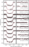 |
Fig. 1 New ground-based transit light curves for HAT-P-23 b. Left: individual photometric time series sorted by the observation date. The best-fitting model is drawn with red lines. A signature of star-spot occultation identified in the light curve acquired on 2021 September 4 is marked with grey points. These measurements were masked out in the transit modelling. Right: photometric residuals from the transit model. |
3.2 Transit timing
Transit timing analysis was performed following the procedure described in Maciejewski et al. (2018). In brief, linear transit ephemerides were refined using the updated sets of mid-transit times. We used the new mid-transit times, which are collected in Table A.2, together with those compiled in Maciejewski et al. (2018, 2020). For homogeneity, we also redetermined the mid-transit times using publicly available light curves reported in the literature since then. Thus, we enhanced our timing datasets with 27 measurements based on data published by Mancini et al. (2022) for KELT-16 b and with 12 measurements from Barros et al. (2022) for WASP-103 b. The de-trended light curves acquired with the CHaracterising ExOplanet Satellite (CHEOPS) were taken in the latter case. The redetermined transit times are also listed in Table A.2. Finally, we used a compilation of 38 mid-transit times for HAT-P-23 b, 39 for KELT-1 b, 103 for KELT-16 b, 125 for WASP-18 b, and 51 for WASP-103 b.
The transit timing datasets were used to refine the linear ephemerides in the form
 (3)
(3)
where E is the transit number counted from the reference epoch T0, taken from the discovery paper. The best-fitting parameters and their 1σ were derived with the MCMC technique based on 100 chains, each of which was 104 steps long, and the first 1000 trials were discarded. Then, the procedure was repeated for a trial quadratic ephemeris in the form
 (4)
(4)
where dPorb/dE is the change of the orbital period between succeeding transits. The Bayesian information criterion (BIC) values were calculated to assess the preferred model. The results are collected in Table A.3. The values of the quadratic terms were found to be consistent with zero within 0.3–1.8σ. The values of BIC also speak in favour of the linear ephemerides for all planets in our sample. The residuals against the refined linear ephemerides are shown in Fig. 6.
Since no statistically significant change of Porb was detected, the fifth percentile of the posterior probability distribution of  was used to place the lower constraint on Q′⋆ at the 95% confidence level. We followed Eq. (5) from Maciejewski et al. (2018). The values of the planet-to-star mass ratio Mb/M⋆ were calculated using the radial velocity amplitudes of the orbital motion Kb following the formula:
 (5)
(5)
where Kb is in m s−1, Pb is in days, and M⋆ is in M⊙. The values of Pb and ib were taken from this study. The values of Kb and come from the most recent redeterminations, which are available in the literature; they are collected together with the references in Table A.4. The errors of the individual parameters were used to estimate the uncertainty for the constraint on Q′⋆. The results are given in Table A.3.
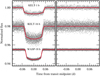 |
Fig. 5 TESS photometric data. Left: phase folded transit light curves for KELT-1 b, KELT-16 b, and WASP-18 b. The best-fitting models are plotted with red lines. Right: photometric residuals from the transit models. |
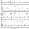 |
Fig. 6 Transit timing residuals for the planets of our sample. The open circles mark the data compiled in Maciejewski et al. (2018, 2020). Open squares are the new literature mid-points redetermined in this study (for Kelt-16 b and WASP-103 b). The filled dots are the new determinations reported in this paper: the green and blue points come from TESS and ground-based photometry, respectively. The uncertainties of the refined ephemerides are illustrated with bunches of 100 lines, each drawn from the Markov chains. |
4 Discussion
For HAT-P-23, Maciejewski et al. (2018) placed the lower constraints on Q′⋆ equal to 5.6 × 10⁵. Then it was refined to (6.4 ± 1.9) × 105 by Patra et al. (2020). Our constraint of Q′⋆ > (2.76 ± 0.21) × 106 is tighter by a factor of ≈4. More recently, Baştürk et al. (2022) have reported 3.8 × 10⁶ but at a higher confidence level of 99%. For WASP-18 b, precise transit timing observations span over 13 yr, making the system the most sensitive probe in the tidal dissipation studies. In the previous study, we eliminated the values of Q′⋆ lower than 3.9 × 10⁶ (Maciejewski et al. 2020). In this study, we push this constraint to Q′⋆ > (1.09 ± 0.04) × 107. In the case of the WASP-103 system, the results of Maciejewski et al. (2018), Patra et al. (2020), and Barros et al. (2022) showed that the orbital period of the giant planet could increase. The presence of a third body in the system or apsidal precession was postulated to explain that finding. Because of that apparently positive derivative of Porb, Maciejewski et al. (2018) and Barros et al. (2022) could place constraints on Q′⋆ only with higher confidence levels: 106 at 99.96% and 1.6 × 10⁶ at 99.7%, respectively. Patra et al. (2020) reported a rather weak constraint with Q′⋆ > (1.1 ± 0.1) × 105 at the 95% confidence level. However, the statistical significance of the reported positive period derivative appears to decrease as the span of observations widens. Our new observations allowed us to place the tighter constraint of  with no statistically significant change in the orbital period of WASP-103 b.
If the mechanism of IGW dissipation operated in the host stars of these three systems, the orbital period shorting could likely be detected in current transit timing data. For HAT-P-23, WASP-18, and WASP-103, the predicted values of Q′IGW are 3.5 × 10⁵, 2.6 × 10⁶, and 4 × 10⁵, respectively (Barker 2020). Our empirical limits on Q′⋆ are greater up to one order of magnitude. As predicted by models of Barker (2020), wave breaking does not happen in these stars, preventing their planets from undergoing rapid orbital decay. KELT-16 b has the shortest observational coverage among our sample objects, which results in the weakest constraint on Q′⋆. Maciejewski et al. (2018) and Patra et al. (2020) reported the consistent values of 1.1 × 10⁵ and (0.9 ± 0.2) × 105, respectively. More recently, Mancini et al. (2022) used the TESS data from Sector 15 and the additional ground-based observations to push this constraint to (2.2 ± 0.4) × 105. Our timing dataset yields a tighter constraint of (2.95 ± 0.23) × 105. This results is still too weak to address tidal boosting because the theoretical prediction is Q′IGW = 7 × 10⁵ (Barker 2020). However, as the mass of the star is ≈1.2 M⊙ (Mancini et al. 2022), this tidal boost is improbable.
The KELT-1 system was recognised as the best candidate for studying the star-planet tidal interaction (Maciejewski et al. 2018) unless the stellar spin is synchronised to the orbital period. The rotation period of the host star was found to be equal to P⋆ = 1.33 ± 0.06 days from the measured projected rotation velocity (Siverd et al. 2012) and P⋆ = 1.52 ± 0.29 days from photometric variations (von Essen et al. 2021). Both results differ by more than 1σ from the orbital period of KELT-1 b, which is 1.22 days. Thus, the spin and orbit synchronisation may still be ongoing. The tidal period in the KELT-1 system is ≈7 days and is longer than half the host star’s rotation. In such a configuration, tidal dissipation might be enhanced by interactions of IWs and turbulent motions in a convective layer of the star. Since an analytic formula that estimates the theoretical value of Q′IW is not available, we utilised Figs. 4 and 6 of Barker (2020) to find Q′IW ≈ 2.6 × 10⁶ for KELT-1. Our empirical constraint of  does not reject this value. We also calculated Q′IGW using Eq. (44) from Barker (2020). Its value of ≈5 × 10⁸ is well beyond the detection limit of current and near-future transit timing observations.
5 Conclusions
Our transit timing data show that tidal dissipation is not boosted by breaking IGWs in HAT-P-23, WASP-18, and WASP-103 host stars. This negative result is in line with the models of stellar interiors of stars with masses above 1.1 M⊙, for which convective cores prevent the waves from reaching the stellar centres and breaking. For KELT-16, the span of observations is not yet long enough to verify the theoretical predictions. Precise transit timing in the following years will allow us to probe the regime of dynamical tides in that system.
The KELT-1 system was found not to be a favourable laboratory for studying tidal dissipation if the EQ tides or IGW mechanisms are considered. However, it might become a unique tool for probing the dissipative tidal interactions of IWs in convective layers. Further observations will help us to explore that scenario.
Acknowledgements
We thank the anonymous referee for the comments that improved the quality of this paper. G.M. acknowledges the financial support from the National Science Centre, Poland through grant no. 2016/23/B/ST9/00579. M.F. and P.J.A. acknowledge financial support from grant PID2019-109522GB-C5X/AEI/10.13039/501100011033 of the Spanish Ministry of Science and Innovation (MICINN) and from grant P20-00737 of the Andalusian Government program PAIDI 2020. M.F., A.S., and P.J.A. acknowledge financial support from the State Agency for Research of the Spanish MCIU through the Center of Excellence Severo Ochoa award to the Instituto de Astrofísica de Andalucía (SEV-2017-0709). M.M. and R.B. acknowledge the support of the DFG priority programme SPP 1992 Exploring the Diversity of Extrasolar Planets (NE 515/58-1 and MU 2695/27-1). This paper includes data collected with the TESS mission, obtained from the MAST data archive at the Space Telescope Science Institute (STScI). Funding for the TESS mission is provided by the NASA Explorer Program. STScI is operated by the Association of Universities for Research in Astronomy, Inc., under NASA contract NAS 5-26555. This research made use of Lightkurve, a Python package for Kepler and TESS data analysis (Lightkurve Collaboration 2018). This research has made use of the SIMBAD database and the VizieR catalogue access tool, operated at CDS, Strasbourg, France, and NASA’s Astrophysics Data System Bibliographic Services.
Appendix A Additional tables
Systemic parameters refined from transit light curves.
Mid-transit times reported in this paper.
Parameters of the refined transit ephemerides.
Literature parameters of the systems under investigation.
References
- Baştürk, Ö., Esmer, E. M., Yalçınkaya, S., et al. 2022, MNRAS, 512, 2062 [CrossRef] [Google Scholar]
- Barker, A. J. 2020, MNRAS, 498, 2270 [Google Scholar]
- Barros, S. C. C., Akinsanmi, B., Boué, G., et al. 2022, A&A, 657, A52 [NASA ADS] [CrossRef] [EDP Sciences] [Google Scholar]
- Brown, D. J. A. 2014, MNRAS, 442, 1844 [NASA ADS] [CrossRef] [Google Scholar]
- Ciceri, S., Mancini, L., Southworth, J., et al. 2015, A&A, 577, A54 [NASA ADS] [CrossRef] [EDP Sciences] [Google Scholar]
- Claret, A. 2017, A&A, 600, A30 [NASA ADS] [CrossRef] [EDP Sciences] [Google Scholar]
- Claret, A., & Bloemen, S. 2011, A&A, 529, A75 [NASA ADS] [CrossRef] [EDP Sciences] [Google Scholar]
- Collins, K. A., Kielkopf, J. F., Stassun, K. G., & Hessman, F. V. 2017, AJ, 153, 77 [Google Scholar]
- Cortés-Zuleta, P., Rojo, P., Wang, S., et al. 2020, A&A, 636, A98 [NASA ADS] [CrossRef] [EDP Sciences] [Google Scholar]
- Fulton, B. J., Shporer, A., Winn, J. N., et al. 2011, AJ, 142, 84 [CrossRef] [Google Scholar]
- Gazak, J. Z., Johnson, J. A., Tonry, J., et al. 2012, Adv. Astron., 2012, 697967 [CrossRef] [Google Scholar]
- Gillon, M., Anderson, D. R., Collier-Cameron, A., et al. 2014, A&A, 562, A3 [NASA ADS] [CrossRef] [EDP Sciences] [Google Scholar]
- Hamer, J. H., & Schlaufman, K. C. 2019, AJ, 158, 190 [Google Scholar]
- Hellier, C., Anderson, D. R., Collier Cameron, A., et al. 2009, Nature, 460, 1098 [NASA ADS] [CrossRef] [Google Scholar]
- Kirk, J., Rackham, B. V., MacDonald, R. J., et al. 2021, AJ, 162, 34 [NASA ADS] [CrossRef] [Google Scholar]
- Lightkurve Collaboration (Cardoso, J.V.D.M., et al.) 2018, Lightkurve: Kepler and TESS time series analysis in Python [Google Scholar]
- Maciejewski, G., Fernández, M., Aceituno, F., et al. 2018, Acta Astron., 68, 371 [NASA ADS] [Google Scholar]
- Maciejewski, G., Knutson, H. A., Howard, A. W., et al. 2020, Acta Astron., 70, 1 [NASA ADS] [Google Scholar]
- Mancini, L., Southworth, J., Naponiello, L., et al. 2022, MNRAS, 509, 1447 [Google Scholar]
- Maxted, P. F. L., Serenelli, A. M., & Southworth, J. 2015, A&A, 577, A90 [NASA ADS] [CrossRef] [EDP Sciences] [Google Scholar]
- Mugrauer, M., & Berthold, T. 2010, Astron. Nachr., 331, 449 [NASA ADS] [CrossRef] [Google Scholar]
- Oberst, T. E., Rodriguez, J. E., Colón, K. D., et al. 2017, AJ, 153, 97 [NASA ADS] [CrossRef] [Google Scholar]
- Patel, J. A., & Espinoza, N. 2022, AJ, 163, 228 [NASA ADS] [CrossRef] [Google Scholar]
- Patra, K. C., Winn, J. N., Holman, M. J., et al. 2020, AJ, 159, 150 [NASA ADS] [CrossRef] [Google Scholar]
- Ricker, G. R., Winn, J. N., Vanderspek, R., et al. 2014, SPIE Conf. Ser., 9143, 914320 [Google Scholar]
- Shporer, A., Wong, I., Huang, C. X., et al. 2019, AJ, 157, 178 [Google Scholar]
- Siverd, R. J., Beatty, T. G., Pepper, J., et al. 2012, ApJ, 761, 123 [Google Scholar]
- Southworth, J., Hinse, T. C., Jørgensen, U. G., et al. 2009, MNRAS, 396, 1023 [NASA ADS] [CrossRef] [Google Scholar]
- Tejada Arevalo, R. A., Winn, J. N., & Anderson, K. R. 2021, ApJ, 919, 138 [NASA ADS] [CrossRef] [Google Scholar]
- von Essen, C., Mallonn, M., Piette, A., et al. 2021, A&A, 648, A71 [NASA ADS] [CrossRef] [EDP Sciences] [Google Scholar]
- Wong, I., Kitzmann, D., Shporer, A., et al. 2021, AJ, 162, 127 [NASA ADS] [CrossRef] [Google Scholar]
The contribution of dissipation in a convective core is predicted to be negligibly small (Barker 2020).
All Tables
All Figures
|
Fig. 1 New ground-based transit light curves for HAT-P-23 b. Left: individual photometric time series sorted by the observation date. The best-fitting model is drawn with red lines. A signature of star-spot occultation identified in the light curve acquired on 2021 September 4 is marked with grey points. These measurements were masked out in the transit modelling. Right: photometric residuals from the transit model. |
| In the text | |
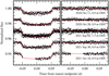 |
Fig. 2 Same as for Fig. 1, but for KELT-1 b. |
| In the text | |
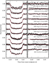 |
Fig. 3 Same as Fig. 1, but for KELT-16 b. |
| In the text | |
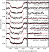 |
Fig. 4 Same as Fig. 1, but for WASP-103 b. |
| In the text | |
|
Fig. 5 TESS photometric data. Left: phase folded transit light curves for KELT-1 b, KELT-16 b, and WASP-18 b. The best-fitting models are plotted with red lines. Right: photometric residuals from the transit models. |
| In the text | |
|
Fig. 6 Transit timing residuals for the planets of our sample. The open circles mark the data compiled in Maciejewski et al. (2018, 2020). Open squares are the new literature mid-points redetermined in this study (for Kelt-16 b and WASP-103 b). The filled dots are the new determinations reported in this paper: the green and blue points come from TESS and ground-based photometry, respectively. The uncertainties of the refined ephemerides are illustrated with bunches of 100 lines, each drawn from the Markov chains. |
| In the text | |
Current usage metrics show cumulative count of Article Views (full-text article views including HTML views, PDF and ePub downloads, according to the available data) and Abstracts Views on Vision4Press platform.
Data correspond to usage on the plateform after 2015. The current usage metrics is available 48-96 hours after online publication and is updated daily on week days.
Initial download of the metrics may take a while.