| Issue |
A&A
Volume 667, November 2022
|
|
|---|---|---|
| Article Number | A118 | |
| Number of page(s) | 13 | |
| Section | Cosmology (including clusters of galaxies) | |
| DOI | https://doi.org/10.1051/0004-6361/202244108 | |
| Published online | 15 November 2022 | |
A bubble size distribution model for the Epoch of Reionization
1
Sorbonne Université, Observatoire de Paris, PSL Research University, CNRS, LERMA, 75014 Paris, France
e-mail: This email address is being protected from spambots. You need JavaScript enabled to view it.
2
Sorbonne Université, UMR7095, Institut d’Astrophysique de Paris, 98 bis Boulevard Arago, 75014 Paris, France
Received:
24
May
2022
Accepted:
29
August
2022
Abstract
Aims. The bubble size distribution is a summary statistics that can be computed from the observed 21-cm signal from the Epoch of Reionization. As it depends only on the ionization field and is not limited to Gaussian information, it is an interesting probe that is complementary to the power spectrum of the full 21-cm signal. Devising a flexible and reliable theoretical model for the bubble size distribution paves the way for its use in astrophysical parameter inference.
Methods. The proposed model was built from the excursion set theory and a functional relation between the bubble volume and the collapsed mass in the bubble. Unlike previous models, it can accommodate any functional relation or distribution. The use of parameterized relations allows us to test the predictive power of the model by performing a minimization best-fit to the bubble size distribution obtained from a high-resolution, fully coupled radiative hydrodynamics simulation known as HIRRAH-21.
Results. Our model is able to provide a better fit to the numerical bubble size distribution at an ionization fraction of xH II ∼ 1% and 3%, as compared to other existing models. Moreover, we compare the relation between the bubble volume and the collapsed mass corresponding to the best-fit parameters, which is not an observable, to the numerical simulation data. A good match is obtained, confirming the possibility of inferring this relation from an observed bubble size distribution using our model. Finally, we present a simple algorithm that empirically implements the process of percolation. We show that it extends the usability of our bubble size distribution model up to xH II ∼ 30%.
Key words: dark ages, reionization, first stars / cosmology: theory / intergalactic medium
© A. Doussot and B. Semelin 2022
 Open Access article, published by EDP Sciences, under the terms of the Creative Commons Attribution License (https://creativecommons.org/licenses/by/4.0), which permits unrestricted use, distribution, and reproduction in any medium, provided the original work is properly cited.
This article is published in open access under the Subscribe-to-Open model. This email address is being protected from spambots. You need JavaScript enabled to view it. to support open access publication.
1. Introduction
The Epoch of Reionization (EoR) is the era when the formation of the first stars and galaxies triggered a major transformation of the intergalactic medium (IGM), whereby the cold and neutral state that follows recombination (at z ∼ 1000) thus transitioned to a warm ionized state. This transition is brought about by the emission of ionizing radiations from the first sources. The resulting ionized bubbles first grow and then percolate until the last islands of neutral hydrogen finally disappear. While the first star in the observable universe may have formed as early as z ∼ 65 (Naoz et al. 2006), the beginning of the reionization process, defined as the time when it becomes observable (through a non-negligible contribution to the Thomson scattering optical depth, the 21-cm signal, or individual high-redshift proto-galaxies) is likely in the z = 15 − 30 range. A more accurate timing depends on the very uncertain formation efficiency of the first stars, which rely on a number of physical processes such as molecular hydrogen formation and dissociation, dynamical feedback from the first supernovae explosions, and a subsequent chemical enrichment of the gas. The end of the process, defined as the complete ionization of the IGM, occurs around z ∼ 5.5 − 6.5 (e.g., Fan et al. 2006; McGreer et al. 2015; Gangolli et al. 2021; Qin et al. 2021; Bosman et al. 2022). Among the many possible probes of the EoR (galaxy luminosity functions, quasar proximity effects, Gamma-ray bursts, Lyman-alpha emitters observations), the 21-cm signal emitted by the neutral IGM holds a unique place. Indeed, rather than sampling the universe on individual lines of sight, it can provide a full 3D tomographic mapping of the EoR (see e.g., Furlanetto & Peng 2006; Mellema et al. 2013). While 21-cm signal statistics such as the global signal or the power spectrum are, in principle, observable with current instruments if systematics are brought under control (e.g., Bernardi et al. 2009, 2010; Ghosh et al. 2011; Yatawatta et al. 2013; Jelic et al. 2014; Asad et al. 2015; Remazeilles et al. 2015; Offringa et al. 2016; Procopio et al. 2017; Line et al. 2017), only the Square Kilometer Array should have sufficient sensitivity to perform tomography at 5′ angular resolution (Koopmans et al. 2015).
The difficulty in interpreting observations of the 21-cm line is that it depends on several local quantities: the gas density, ionization fraction, kinetic temperature and velocity, and the local flux in the Lyman-alpha line for coupling the spin temperature to the kinetic temperature. These values are, in turn, determined by non-local and non-linear processes: mainly gravity and radiative transfer, but also all the processes that regulate the formation of the sources of radiations. Consequently, it is necessary to build parameterized models that are theoretical, semi-numerical, or numerical that would attempt to account for all these effects and explore the parameter space in the hope of matching the observed signal. Obviously, the methodology to explore the parameter space efficiently (beyond brute-force gridding) has been an active field of research. For example, Pober et al. (2014) used the Fisher matrix formalism in combination with the 21cmFAST semi-numerical code (Mesinger et al. 2011) to estimate the constraints that can be obtained from future observations with the HERA interferometer. Greig & Mesinger (2015, 2017, 2018) deployed a full Bayesian Markov chain Monte Carlo (MCMC) framework, which is also based on 21cmFAST, to compute the full posterior distribution for the model parameters. Since even the use of a semi-numerical model at low resolution in conjunction with a MCMC approach represents a significant computational cost, some authors have explored the use of emulators of the semi-numerical model, using Gaussian processes (Kern et al. 2017) or neural networks (Schmit & Pritchard 2018; Jennings et al. 2019; Cohen et al. 2020; Bye et al. 2022; Bevins et al. 2021). Another avenue of research consists of training supervised learning algorithms to perform the inverse modeling to retrieve the model parameters from the signal (Shimabukuro & Semelin 2017; Gillet et al. 2019; Doussot et al. 2019; Hassan et al. 2020; Zhao et al. 2022a,b; Prelogović et al. 2021). While these works have been limited to maximum likelihood-type inference, the posterior distribution could, in principle, be accessed using a Bayesian neural network (see, e.g., Hortúa et al. 2020) or with density estimators that also use neural networks for dimensionality reduction (Zhao et al. 2022a).
Most of these parameter inference studies use the 21-cm signal power spectrum as a metric of the difference between the model and reality, either as a proof of concept (as in the above references) or based on the existing upper limits (Mondal et al. 2020; Ghara et al. 2020, 2021; Greig et al. 2021a,b; Abdurashidova et al. 2022). Others have used the global signal (e.g., Monsalve et al. 2019) or, as a proof of concept only, they have used the full tomography (e.g., Gillet et al. 2019; List & Lewis 2020; Zhao et al. 2022a). When the study is based on the global signal or the power spectrum, fluctuations induced by the ionization fraction, the X-ray heating, and the Lyman-α coupling are mixed. It is only at times when one type dominates over the others that we can hope to isolate it. Tomography, on the other hand, offers the possibility to disentangle the different contributions, for example, by identifying individual ionized bubbles. However, as it is not summary statistics, it suffers from a high level of thermal noise. This is why a summary statistics derived from the tomography and associated with a single source of fluctuation such as the bubble size distribution (BSD), which depends only on the ionization field, may be an interesting metric for parameter inference. It would likely provide constraints on the parameter space with different degeneracies than the 21-cm power spectrum, for example. It is also sensitive to the non-Gaussian information in the signal. While instrumental limitations, starting with the increasing thermal noise at higher angular resolution (e.g., Mellema et al. 2013), will affect the process, methods for obtaining the bubble size distribution from tomographic observations have been explored (Giri et al. 2018; Bianco et al. 2021). Semi-numerical, or even numerical simulations, could then be used to perform parameter inference studies based on this quantity. If an accurate theoretical model can indeed be devised, however, it stands a good chance of involving a lower computational cost during the inference process.
To our knowledge, there exists currently only one theoretical model: it is described in Furlanetto et al. (2004, hereafter FZH04) and relies on the excursion set theory (see also Paranjape & Choudhury 2014; Paranjape et al. 2016 for some improvements to the model). The FZH04 model has been tested against numerical simulations in Mesinger & Furlanetto (2007) and Lin et al. (2016), who found some level of discrepancy. The fundamental assumption in the FZH04 model is that the mass of the ionized gas in each bubble is uniquely determined and directly proportional to the collapsed halo mass in the bubble. This is actually a necessary assumption for the model to be able to deliver an analytic formula. While this assumption is natural, it is also simplistic. Indeed, environmental effects such as source clustering, inhomogeneous recombination, or external photo-evaporation, are bound to introduce some scattering into the one-to-one relation, but also induce a non-linear relation. Another limitation of the model is associated with the percolation process. Indeed, the excursion set formalism evaluates the probability for a region to be ionized, but does not account for the possibility that such regions overlap. Furlanetto & Oh (2016) have studied the process of percolation for the ionization field and shown that an ionized region with infinite volume (that is extending from one side of the box to the other in simulations) appears as soon as the average ionized fraction reaches xH II ∼ 0.1. There is no framework in the FZH04 model to account for percolation.
In this work, we present an alternative, more flexible theoretical model to describe the BSD. By reverting to the original Press-Schechter spirit rather than using the excursion set theory, we lose something in terms of formal rigor, but we gain much in term of flexibility. Not only are we able to consider any functional relation between the ionized gas mass and collapsed halo mass, but we can also move from a one-to-one relation to a distribution characterized by its average and dispersion. We aim to show that this more flexible representation offers a good match to the result of a high-resolution numerical simulation. Then, a choice of an astrophysically motivated parameterization for the relation opens the way for parameter inference using the BSD as a metric.
In Sect. 2, we present our methods: the reference numerical simulation, the algorithm for computing the numerical BSD and our proposed theoretical model. In Sect. 3, we test the predictive power of the model by performing a best fit of the theoretical model parameters to the numerical BSD. The resulting ionized-gas volume to collapsed-mass relation that corresponds to the best-fit parameters is then compared to the same relation directly computed from the simulation data. Section 4 evaluates the improvements produced by including a dispersion in the relation. Section 5 presents and evaluates the performances of an empirical percolation algorithm. Finally, in Sect. 6, we give our conclusions.
2. Bubble size distribution: Numerical computation and analytical models
2.1. The HIRRAH-21 simulation
High Resolution Radiative Hydrodynamics simulation for 21-cm (HIRRAH-21) is a simulation based on the LICORICE code, as detailed in Baek et al. (2009; see Baek et al. 2010; Semelin 2016 for subsequent upgrades). LICORICE computes the evolution of gas, dark matter, and radiation on cosmological scales. It is a particle-based code modeling the dynamics using the Tree-SPH method (and references therein Semelin & Combes 2002). The dynamics is fully-coupled to the radiative transfer of ionizing UV and X-ray using the Monte Carlo scheme described in Baek et al. (2009, 2010). Notable features easily implemented in the Monte Carlo approach include: the photons being propagated with the correct speed of light on an adaptive grid, with cosmological redshifting included. This is especially relevant when handling X-rays, which can travel long distances prior to absorption.
HIRRAH-21 is meant to complement the 21SSD set of simulations presented in Semelin et al. (2017). The set’s 21-cm signal predictions are publicly available1. The initial conditions for HIRRAH-21 were produced with the MUSIC package (Hahn & Abel 2011), using the same random seeds as for the 21SSD simulations for the shared resolution levels, along with a new one for the additional resolution level in HIRRAH-21 (see below). Thus, the initial density field in HIRRAH-21 differs from those in 21SSD only by fluctuations at the newly resolved scales. For reference, the X-ray production parameters are fX = 1 and rH/S = 0.5 (see Semelin et al. 2017 for definitions), although in this work, where we focus on the ionized bubbles size distribution, such moderate values have little impact on the results.
HIRRAH-21 follows the evolution of 20483 particles, half of them baryons and the other half dark matter, in a 200 h−1 cMpc box. A parallelized halo finder based on a friend-of-friend (FoF) scheme resolves halos down to 4 × 10⁹ M⊙ (i.e., 20 dark matter particles). The dynamicalimestep is 0.5 Myr (divided by 3 at an expansion factor smaller than 0.03) and the gravitational softening is ϵ = 2 ckpc. The parameters of star formation and the ionizing photon escape fraction are the same as in 21SSD, yielding an earlier reionization history due to the better mass resolution for halos. The spectral properties of the sources are also the same as in 21SSD, resulting from a Salpeter initial mass function truncated at 1.6 M⊙ and 120 M⊙. Roughly 5 × 10¹¹ Monte Carlo photon packets were propagated during the simulation, with 7 × 10¹⁰ in-flight photons by the end of reionization, which occurs around z ∼ 6.9.
For reference, we show in Fig. 1, the volume-weighted ionized (purple) and neutral (orange) fractions as functions of the redshift from the HIRRAH-21 simulation. The optical depth obtained from this simulation is τ ∼ 0.0692. We use a standard Λ-CDM cosmology with parameter values in accordance with Planck Collaboration XIII (2016): H0 = 67.8 km s−1, ΩM = 0.308, Ωb = 0.0484, ΩΛ = 0.692, σ8 = 0.8149, and ns = 0.968. The HIRRAH-21 simulation was performed on 16386 CPU cores using 4096 MPI domains and required ∼3 × 10⁶ CPU hours.
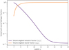 |
Fig. 1. Volume-weighted ionized (purple) and neutral (orange) fraction as a function of the redshift from the HIRRAH-21 simulation. |
2.2. Numerical computation of the bubble size distribution
To identify ionized bubbles in HIRRAH-21, we use a FoF method, based on the ionization field interpolated on a 10243 grid. It means that we can detect bubbles with a characteristic size of ≳288 ckpc. We tag as ionized any cell that has an ionization fraction above a given threshold,  . A bubble is a connected set of ionized cells. A similar algorithm has been used and analyzed in previous studies (Friedrich et al. 2011; Furlanetto & Oh 2016; Giri et al. 2018).
When the bubble is identified, we can compute its volume as:  where Vcell is the volume of one cell, Ncell is the number of cells in the considered ionized bubble, and xH II,i is the ionization fraction of cell, i. If necessary, we can then compute an equivalent radius from the volume assuming a spherical shape. Other methods such as the mean-free-path or the spherical-average methods give similar but not strictly equivalent results (Mesinger & Furlanetto 2007; Zahn et al. 2007; Giri et al. 2018).
We subsequently produced a list of bubble volumes which can easily be converted into a number density of bubble in an interval of radius, [r, r + dr]: nb(r)dr. In accordance with previous works (Furlanetto & Oh 2016; Giri et al. 2018), to depict the bubble size distribution, we use the quantity  . This quantity measures the fraction of space occupied by ionized bubbles with volume V in a given logarithmic bin of volume dlnV. This is equivalent to the probability density function
  given in some works (Furlanetto et al. 2004; Lin et al. 2016; Giri et al. 2019) up to a constant of
  , where Q is the global volume-filling fraction of ionized regions.
In Fig. 2, we show the bubble size distribution from our HIRRAH-21 simulation at average ionization fractions of xH II ∼ 1%, 3%, 10%, and 20%, which in our simulation correspond, respectively, to redshifts z ∼ 9.8, 9.3, 8.5, and 8.1, for ionization thresholds:  (solid lines) and 0.8 (dashed lines). At high volumes (V ≳ 10 cMpc3), the distribution drops for xH II ∼ 1% and 3% because we consider very early stages of reionization when bubbles have not yet had time to grow. The distribution is more or less flat for xH II ∼ 10%, and it drops again for xH II ∼ 20%. The decrease in amplitude after xH II ∼ 10% is theoretically expected because of the percolation process that merges large bubbles into a single one spanning a whole simulation box (Furlanetto & Oh 2016). The average ionization value at which this percolated cluster forms seems to be only weakly model-dependent, as shown in Furlanetto & Oh (2016). In our case, it appears at xH II ∼ 10%. For smaller bubbles (V ≲ 5 cMpc3), the finite resolution of our simulation affects the results leading to a depletion in the number of detected bubbles.
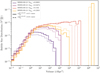 |
Fig. 2. Bubble size distribution from the HIRRAH-21 simulation at global ionization fractions xH II ∼ 1%, 3%, 10%, and 20% for ionization thresholds, |

Figure 2 also shows that the BSD obtained for  is similar to the one using a threshold of 0.5, with a slightly delayed evolution. This is understandable as the threshold value simply modifies our definition of what is part of the ionized bubbles but does not affect the physical processes that rule their evolution. The exact same bubble will have, at the same redshift, an estimated volume smaller in the
  case than in the
  case or, equivalently, a volume that was reached somewhat earlier in the
  case. We note, however, that the changes in the BSDs created by changing the threshold value are smaller than those created by the evolution between two of our sampled average ionization fractions and would thus correspond to very small shifts in the timing of the ionization history. Moreover, the parameters that are inferred from the BSD (described in Sect. 3) do not seem to evolve much. Thus, in the following, we only use
  .
.
2.3. Excursion set based model of the bubble size distribution
An analytical model used to compute the bubble size distribution was proposed by Furlanetto et al. (2004, already referred to as FZH04), based on the assumption that the mass of the gas in an ionized region is directly proportional to the mass of the collapsed objects inside the region, with the proportionality factor called the efficiency factor, ζ. We refer to FZH04 for the full details of the model. The end result is that the bubble size distribution is expressed analytically as :
![Mathematical equation: $$ \begin{aligned} m\frac{\mathrm{d}n}{\mathrm{d}m}=\sqrt{\frac{2}{\pi }}\frac{\overline{\rho }}{m}\left|\frac{\mathrm{d}\ln \sigma }{\mathrm{d}\ln m}\right|\frac{B_{0}}{\sigma (m)}\exp \left[-\frac{B^{2}(m,z)}{2\sigma ^{2}(m)}\right] ,\end{aligned} $$](/articles/aa/full_html/2022/11/aa44108-22/aa44108-22-eq13.gif) (1)
(1)
where m is the ionized gas mass in the bubble, dn is the number density of bubbles with gas mass between m and m + dm,  is the mean density of the universe, σ(m) is the mass variance of the linear density field, and B(m, z) = B0 + B1σ2(m) is a linear fit to the overdensity threshold; the latter is required so that the collapsed fraction in the region is sufficient to ionize it. To enable a comparison with our own model, we convert the mass dependency of the distribution in Eq. (1) into a size dependency, based on the relation:

Using a formalism derived from the extended Press-Schechter theory, this model relies on the assumption that the mass of ionized gas depends linearly on the mass of collapsed objects to produce an analytical formulation for the BSD. Thus, it cannot take into account another functional relation nor any dispersion in the relation.
2.4. A new, flexible model for the bubble size distribution
2.4.1. Computing the conditional mass function
Our model for computing the BSD aims at using a flexible physical prescription to relate, for a given “ionized” region, the amount of mass bound in self-gravitating objects (i.e., the collapsed mass) to the volume of the region. So, the first task is to describe the population of collapsed objects in a given region of the universe. Since ionized bubbles typically form in overdense regions, we cannot simply use the formalism of the halo mass function (HMF), but we must resort to the conditional mass function (CMF) first presented in Lacey & Cole (1993, 1994).
We go on to consider a region of volume V0, mass  and mass variance σ0 = σ(M0). In the following study, σ(M) is computed using THEHALOMOD online calculator (Murray et al. 2013, 2021). By construction, our model can use any form for the conditional mass function. In this study we will mainly use the conditional mass function derived from the empirical best-fitting halo mass function of Sheth & Tormen (1999). For a region with overdensity δ0, the CMF can be written as (Rubiño-Martín et al. 2008):
![Mathematical equation: $$ \begin{aligned} n_{\text{ c,ST}}=\sqrt{\frac{2}{\pi }}\frac{\overline{\rho }}{m}\left|\frac{\mathrm{d}\sigma }{\mathrm{d}m}\right|\frac{\sigma (m)\left|T(\sigma ,\sigma _{0}) \right|}{(\sigma (m)-\sigma _{0})^{\frac{3}{2}}}\exp \left[-\frac{(B_{\text{ ec}}(\sigma ,z)-\delta _{0})^{2}}{2(\sigma (m)-\sigma _{0})^{2}}\right] ,\end{aligned} $$](/articles/aa/full_html/2022/11/aa44108-22/aa44108-22-eq17.gif) (2)
(2)
where
with Bec the barrier derived by Sheth et al. (2001) and given by
![Mathematical equation: $$ \begin{aligned}B_{\text{ ec}}(\sigma ,z)=\sqrt{0.707}\delta _{c}(z)\left[ 1+0.485\left( \frac{0.707\delta _{\rm c}(z)^{2}}{\sigma ^{2}} \right)^{-0.615}\right].\end{aligned} $$](/articles/aa/full_html/2022/11/aa44108-22/aa44108-22-eq19.gif)
In Sect. 4.3, we compare the results with those for the CMF derived in the extended Press-Schechter formalism (Press & Schechter 1974; Bond et al. 1991; Lacey & Cole 1993, 1994) to highlight our model sensitivity to this initial choice for the CMF. This other form of the conditional mass function can be written as:
![Mathematical equation: $$ \begin{aligned} n_{\text{ c,EPS}}=\sqrt{\frac{2}{\pi }}\frac{\overline{\rho }}{m}\left|\frac{\mathrm{d}\sigma }{\mathrm{d}m}\right|\frac{\sigma (m)(\delta _{c}-\delta _{0})}{(\sigma (m)-\sigma _{0})^{\frac{3}{2}}}\exp \left[-\frac{(\delta _{c}-\delta _{0})^{2}}{2(\sigma (m)-\sigma _{0})^{2}}\right] ,\end{aligned} $$](/articles/aa/full_html/2022/11/aa44108-22/aa44108-22-eq20.gif) (3)
(3)
where δc = 1.686.
2.4.2. Collapsed mass probability distribution
As long as the non-Gaussianities resulting from non-linear structure formation have not had time to develop on the scale of the considered region, the probability density function for a region of volume V0 to have an overdensity δ0 is given by:
 (4)
(4)
Then, the collapsed mass probability density for a region of volume V0 can be expressed as a marginalization over δ:
 (5)
(5)
where PV0(Mcoll | δ) is the conditional probability for a region of volume V0 to have a collapsed mass Mcoll, knowing that it has an overdensity δ. In the CMF formalism this conditional probability is a Dirac distribution: the collapsed mass is uniquely determined by the volume and overdensity of the region. This collapsed mass is however only an average value for all regions with identical volume and overdensity. A sample variance of the density field within each region will generate a distribution of values around this average. Thus, we explored two ways to model PV0(Mcoll | δ):
The simplest approach is to use the average value from the CMF formalism. In this case we can directly compute the collapsed mass using a generic conditional mass function nc:
 (6)
(6)
The minimum mass threshold Mmin is necessary in our case since we are interested only in halos that can efficiently form stars and thus produce ionizing photons. It can be set, for example, at the atomic cooling limit, ∼1 × 10⁸ M⊙, or at the resolution limit of a simulation, allowing our model to fit results in various frameworks. For this study, we set Mmin ∼ 4 × 10⁹ M⊙ to correspond to the resolution limit of the HIRRAH-21 simulation. With this assumption, the conditional probability of PV0(Mcoll | δ) is:

where δD is the Dirac distribution and we can rewrite the collapsed mass distribution inside regions of volume, V0, of Eq. (5) as:
 (7)
(7)
The more realistic approach is to consider that regions of the same size and average overdensity can have a distribution of collapsed masses. A simple way to take the sample variance within each region into account is to model the number of objects in each mass bin using a Poisson distribution (Barkana & Loeb 2004). We note that since we are not interested simply in the total number of collapsed objects but, rather, in the total mass in collapsed objects, we cannot work with a single mass bin, relying on the fact that the sum of two independent Poisson distributed random variables is Poisson distributed: indeed, this property does not work for a linear combination of independent random variables (the total collapsed mass in our case).
The Poisson distribution of the number of halos in a region of volume, V0, and overdensity, δ*, with a mass in the range of [M*, M* + dM], must have an expected value equal to the average number of halos in this range as predicted by the conditional mass function: V0nc(M*, δ*)dM. This is sufficient to fully define the Poisson distribution. Therefore, we can numerically construct the distribution PV0(Mcoll | δ*) with a Monte Carlo sampling approach. In each mass bin, we draw the number of halos from the correct Poisson distribution, then we combine these values to compute the total collapsed mass, and iterate the process many times to build the total collapsed mass distribution. Since these distributions depend on two parameters (V0 and δ*), it is useful to tabulate them in advance. We can finally apply Eq. (5) to get the collapsed mass distribution marginalized over the overdensity.
Figure 3 represents the collapsed mass distribution computed at redshift z ∼ 9.8 including (dashed lines) the sample variance or without including it (solid lines) and using a CMF either from Eq. (3) (purple) or Eq. (2) (yellow) for various ionized regions sizes. The main difference induced by sample variance is for values of collapsed mass of ≲1010 M⊙, namely, values that are close to our simulation mass resolution of 4 × 10⁹ M⊙. This is expected since in the cases when many bin are populated with halos (thus yielding a large collapsed mass), the central limit theorem applies and the distribution peaks around this average. In addition, since at a given size, ionized regions are likely to be regions with a large amount of collapsed mass, it is only the right-end of the distributions that are relevant for the BSD computation. In this range, the expected difference between BSD computed with or without the sample variance is significant for the smallest ionized bubbles, where only a few halos are present in the region. The low mass oscillations that can be seen in the cases when the Poisson distribution is used are generated by using a sharp lower mass limit for halos. Indeed, between Mmin and 2 × Mmin the region contains at most one halo, with decreasing probability toward larger mass (as dictated by the CMF). When the collapsed-mass reaches 2 × Mmin, suddenly configurations with two halos become possible, creating a sharp rise in the probability. Such a phenomenon occurs again, with decreasing amplitude, when integer numbers of Mmin are reached.
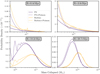 |
Fig. 3. Collapsed mass distribution computed at redshift z ∼ 9.8 (corresponding to xH II ∼ 1%) considering the sample variance (dashed lines) or not (solid lines) using the conditional mass function of Eq. (3) (purple) or of Eq. (2) (yellow). The results are shown for ionized regions of radius of: 0.4 cMpc, 3 cMpc, 10 cMpc, and 20 cMpc. |
In Fig. 3, we also see that the collapsed mass probability distribution peak is shifted to lower collapsed mass when using the CMF based on Press & Schechter (1974) compared to the Sheth & Tormen (1999) case, thereby showing the effect on the collapsed mass probability distribution of this well-known difference between the two theories (Sheth & Tormen 1999; Rubiño-Martín et al. 2008). This difference impacts the resulting BSD, as we discuss later in this work.
2.4.3. Parameterizable bubble size distribution
Having computed the collapsed mass distributions for a wide range of region volumes using Eq. (5), we can now express the probability for a region of volume V0 to be ionized as:
 (8)
(8)
where  is computed from the physical relation Mcoll(Vion) that links the volume of an ionized bubble with the collapsed mass it contains. We note that this relation cannot be derived from an HMF formalism since it must implement the condition that the region is ionized. One of the key properties of our model is that it allows us to use various physical relations based on theory or simulations results alike. We will investigate different functional relations. The final step to compute the BSD is to write the number per unit volume of ionized bubbles with volume between V and V + dV as:
 (9)
(9)
This last step is very much in the spirit of the original Press-Schecher theory (even if we do not rely on the corresponding halo mass function). What it lacks in rigour, it gains in flexibility in the Mcoll(Vion) relation. The FZH04 model follows the more rigorous approach of the extended Press-Schechter formalism, but it is limited to a linear Mcoll(Vion) relation, which is the only case where an analytical solution to the diffusion equation is known.
2.4.4. Accounting for dispersion in the Mcoll(Vion) relation
If the physical relation between the ionized bubble volume and the collapsed mass in the bubble displays a non-negligible dispersion, as for our HIRRAH-21 simulation, we can account for it. Given the collapsed mass distribution for a region of a volume V0, we use the distribution characterizing the collapsed mass dispersion at this same volume PV0, ion(Mcoll) to obtain a modified distribution encapsulating this scatter :
 (10)
(10)
It is worth noting that although we will suppose a Gaussian behaviour for our following study, the dispersion distribution can theoretically take any form, be it analytical or numerical. Applying Eq. (9) to our new distribution, we can now compute a bubble size distribution corresponding to a physical relation with dispersion PV0, ion(Mcoll).
2.4.5. Model summary
For the sake of clarity, we hereby sum up the main computation steps of our model. We compute the number per unit volume nb(V0) of ionized regions of volume V0 as follows:
We first compute PV0(δ0) which is the probability density function for a region of volume V0 to have an overdensity δ0 using Eq. (4). We then compute PV0(Mcoll | δ) the conditional probability for a region of volume V0 to have a collapsed mass Mcoll knowing that it has an overdensity δ. This can be done in two ways: (1) assuming that the numerical sample variance effect within ionized regions is negligible it can be computed using a Dirac distribution and the CMF formalism (Eq. (6)); (2) taking into account the sample variance effect implies to numerically construct PV0(Mcoll|δ) using a Poisson distribution and a Monte Carlo sampling as detailed in Sect. 2.4.2.
We then marginalize over δ to obtain the collapsed mass probability density PV0(Mcoll) for a region of volume V0 using Eq. (5). We define a parameterized physical relation Mcoll(Vion) that connects the volume of a ionization bubble with the collapsed mass it contains. This can be a one-to-one relation or a distribution. The probability of a region of volume V0 to be ionized Pion(V0) is then computed differently depending on the case: (1) using Eq. (8) if the Mcoll(Vion) is one-to-one or (2) if a dispersion is assumed, the functional form of its variance has to be defined. We then access Pion(V0) by marginalizing over the collapsed mass distribution (now approximated by its mean and variance) using Eq. (10). Finally, the number per unit volume of ionized bubbles with volume between V and V + dV is given by Eq. (9).
3. Testing the model for parameter inference
3.1. Physical relation between the collapsed mass inside an ionized region and its volume
To compare our model with the numerical results of the HIRRAH-21 simulation, we selected two functional forms to parameterize the relation between the volume of an ionized region and its collapsed mass content. A simple physical insight would lead us to consider Mcoll ∝ Vion: the ionized volume is proportional to the number of emitted photons, itself proportional to the collapsed mass assuming a linear mass-to-luminosity relation. Nevertheless, we initially chose to consider a more general  relation, a liberty that we withdraw later on.
3.1.1. Power law relation
The first and most straightforward choice is to assume a power law relation which can be expressed as:
 (11)
(11)
where α and A are two parameters to be fitted. While convenient, this first parameterization will not be able to handle the effect of the mass resolution and should be limited to a range of volumes which is not affected by this limit, that is, a volume, Vion, such that  , where Mmin = 4 × 10⁹ M⊙ in our case.
3.1.2. Logarithmic softplus
To better fit the simulations and observations, we want to be able to account for the effect of the lower mass limit for star forming halos that exists physically, although at a lower mass than our simulation mass resolution limit. This physical limit is set by the temperature floor that can be reached by hydrogen atomic or molecular cooling. This suggests another parameterization that will be able to account for this change of regime (at the cost of a higher number of free parameters).
In HIRRAH-21, the mass limit, Mmin, is the result of the resolution limit. It induces a sharp threshold in mass and so a flat Mcoll(Vion) relation at low volumes. This is very much model dependent: for instance, Cohen et al. (2016) considered three regimes of star formation efficiency depending on the halo mass. For our simulation, a possible choice for a function that must be flat in a given range (as the collapsed mass cannot be smaller than Mmin) and linear above a given threshold is the rectifier linear function, better known as ReLu in the artificial intelligence domain and defined as y : x ↦ αmin(x − xth, 0)+yth with α, xth, and yth three free parameters and, in our case, y ≡ log10(R) and x ≡ log10(Mcoll). However, this function is piece-wise linear and numerical computation around the breakpoint tends to result in a brutal and artificial drop in the amplitude of the output BSD. For this reason we chose to implement a variation of this function without any breakpoints: the logarithmic Softplus, as follows:
![Mathematical equation: $$ \begin{aligned} \log _{10}\left(\frac{M_{\rm coll}}{M_{\rm coll,th}}\right) =\alpha \frac{\ln \left( 1+\exp \left[k\log _{10}\left(\frac{V_{\text{ ion}}}{V_{\text{ th}}}\right)\right]\right)}{k} ,\end{aligned} $$](/articles/aa/full_html/2022/11/aa44108-22/aa44108-22-eq33.gif) (12)
(12)
where α is the slope of the relation at high volume, k = 10 is the smoothness of the transition from one regime to the other and Mcoll, th and Vth are the collapsed mass and corresponding volume at the transition from the regime dominated by the mass limit to a regime where it is negligible. We set k = 10, since the sharpness of the transition is not critical for this proof-of-concept study, meaning that this parameterization effectively relies on three parameters.
3.2. Parameter inference
One key application of the model developed in this study is that it can be used to infer the relation Mcoll(Vion) from the BSD and thus to constrain the underlying astrophysical processes. For that, one has to assume a parametric form for the relation and apply optimization algorithms such as gradient-descent or Markov chain Monte Carlo (MCMC) to fit a given observed BSD. For this study, we apply a simple grid-search method to illustrate the capabilities of this model. To quantify the error, we use a mean squared error on the logarithm of the quantities which can be written as:
 (13)
(13)
where ytrue is the reference value. In our case, ytrue is always the numerical value computed from HIRRAH-21 simulation. We first focus on low global ionization fractions (xH II ∼ 1% and xH II ∼ 3%) where the effect of percolation is negligible.
In Fig. 4, we use both of our power law (green lines) and Softplus (orange lines) parameterization, with (dashed lines) and without (solid lines) sample variance modeled by the Poisson distribution. We fit the BSD from the HIRRAH-21 simulation (gray histogram) to infer the parameters. The method is applied at two different global ionization fraction of xH II ∼ 1% (left panel) and xH II ∼ 3% (right panel). We also show the best-fit FZH04 model for reference. We see that all our best fits are reasonably close to the numerical distribution. Table 1 presents the resulting mean squared errors for the BSD best-fit ![Mathematical equation: $ \mathrm{MSE}\left(\log_{10}\left[V^{2}\frac{\mathrm{d}n_{\mathrm{b}}}{\mathrm{d}V}\right]\right) $](/articles/aa/full_html/2022/11/aa44108-22/aa44108-22-eq35.gif) and of the corresponding reconstructed Mcoll(Vion) relations compared to the numerical relation MSE(log10[Mcoll(Vion)]), for both xH II ∼ 1% and xH II ∼ 3%. For all the current models, it shows that the fit mean squared error is, at worst, 17% but always under 10% for the Softplus parameterization.
and of the corresponding reconstructed Mcoll(Vion) relations compared to the numerical relation MSE(log10[Mcoll(Vion)]), for both xH II ∼ 1% and xH II ∼ 3%. For all the current models, it shows that the fit mean squared error is, at worst, 17% but always under 10% for the Softplus parameterization.
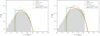 |
Fig. 4. Various fit of the reference numerical BSD (gray histogram) using a power law parameterization from Sect. 3.1.1 (green lines) or a logarithmic Softplus parameterization from Sect. 3.1.2 (orange lines) considering the sample variance (dashed lines) or otherwise (solid lines). A numerical fit of the reference BSD from Furlanetto et al. (2004; Eq. (1)) using only the efficiency parameter ζ is shown as a comparison (yellow dashed line). The fit is done at xH II ∼ 1% (left panel) and xH II ∼ 3% (right panel). |
![Mathematical equation: $ \mathrm{MSE}\left(\log_{10}\left[V^{2}\frac{\mathrm{d}n_{\mathrm{b}}}{\mathrm{d}V}\right]\right) $](/articles/aa/full_html/2022/11/aa44108-22/aa44108-22-eq36.gif)
However, the theoretical BSD seems to overestimate the total ionization fraction as illustrated by their respective maximums that have an amplitude that is about 50% greater than the numerical one. As expected, the decreasing population of ionized bubbles with decreasing volume due to the mass resolution limit is better fitted when using the Softplus model and the overall shape appears to be closer to the numerical reference. Our model also gives results closer to the numerical distribution for all cases than the FZH04 model, especially at volumes of V ≲ 102cMpc3.
Fitting the relatively smooth shape of the numerical BSD with two- and three-parameter models is not in itself a strong result. The fact that the parameters and the model are based on a physical understanding of the system is more interesting; however, showing that the inferred values for the parameters yield a Mcoll(Vion) relation that actually matches what we can directly compute from simulations data would tell us that when we apply this procedure to an observed BSD, we will learn something relevant about the process of reionization. We show in Fig. 5, for both xH II ∼ 1% (left panel) and xH II ∼ 3% (right panel), the inferred physical relation Mcoll(Vion) for the power law (green lines) and Softplus (orange lines) parameterizations, with (dashed lines) and without (solid lines) considering the sample variance, and the distribution for the same relation computed directly with the data from the simulation. We see that all parameterizations infer relatively reasonable physical relations. However all our inferred relations overestimate the average amount of collapsed mass inside a region of a given volume, especially for the smallest volumes (V ≲ 2 × 101 cMpc3), compared to the average value directly computed from the simulation. Referring to Table 1, it leads to a Mcoll(Vion) mean squared error of ∼5% for models considering the sample variance and ∼2.5% for the others.
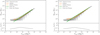 |
Fig. 5. Collapsed mass inside an ionized region as a function of its volume. The gray colormap represents the distribution of halos the HIRRAH-21 simulation and its numerical mean (top panel) and dispersion (bottom panel) are shown as black lines in the corresponding panels. The inferred relations with (dashed lines) and without (solid lines) considering the sample variance are shown for both our power law (green lines) and our logarithmic Softplus (orange lines) parameterizations. The fit is done at xH II ∼ 1% (left panel) and xH II ∼ 3% (right panel). |
This difference must be tempered by the possible uncertainties in both the simulation and the model results. Concerning HIRRAH-21 simulation, a FoF algorithm is run on the particle distribution to construct halos. This halo finder especially relies on a linking length that roughly quantify the maximal distance for two particles to be considered as neighbours inside the same halo (Davis et al. 1985). Various values of the linking length can be considered reasonable and choosing one rather than another impacts the resulting Mcoll(Vion) relation. For the analytical model, it has been specifically designed to be adjustable and we show in Fig. 3 that the collapsed mass probability already differs by a factor of 2 between the two depicted halo mass function formalisms. The inferred Mcoll(Vion) can therefore vary for two different CMFs.
In Fig. 4, we see that the difference induced by including the sample variance is relatively negligible in our case. In terms of physical relation inference, Fig. 5 and Table 1 show that models that include sample variance show worse performance than the others, as they are less in agreement with the numerical mean relation. It is possible that the sharp mass cutoff considered in the Poisson distribution approach is a poor description of the actual mass resolution limit in the simulation. Consequently, although it is theoretically more comprehensive to account for this effect, we will from now on only look at cases where the sample variance is not considered. Furthermore, for all cases the slope α of our mean relation in Eqs. (11) and (12) is always close to the expected value of 1. Going forward, we fix it at this value, effectively withdrawing one free parameter from both mean relations.
4. Injecting dispersion in the Mcoll(Vion) relation
In Sect. 3, we show that for both of our parameterizations, our best-fit BSD have a moderate deficit of large bubbles and excess of mid-sized bubbles. This problem could be partially solved if we consider a dispersion in the physical Mcoll(Vion) relation. In our numerical simulation, this dispersion does exist and is non-negligible, as can be seen in Fig. 5. The effect of this dispersion could be important considering that a variation of the mean Mcoll results in a strong variation in term of collapsed mass probability distribution, as we can see in Fig. 3.
4.1. Dispersion parameterizations
As we detail in Sect. 2.4.4, the model requires a modification to include dispersion in the Mcoll(Vion) relation. We now need to choose a parameterization. As shown in Fig. 5, the dependence of the standard deviation as a function of Vion exhibits two different trends depending on the dominance of the mass resolution effect. However, the slopes are not sharp and to avoid adding too many free parameters, we decided to use the following simple parameterization:
 (14)
(14)
with B and β as our free parameters. Since we set α to 1 in the mean relation, by using Eq. (14) along with the mean relations of Eq. (11), we can fit a total of three free parameters while with Eq. (12) we will be using four free parameters in total.
4.2. Fitting the bubble size distribution with models including dispersion
In Fig. 6, we used both of our parameterizations detailed in Sects. 3.1.1 (green lines) and 3.1.2 (orange lines) with (dashed lines) and without (solid lines) considering dispersion. We fit the BSD from the HIRRAH-21 simulation (gray histogram) to infer the underlying parameters of this parameterizations. The method is also applied at two different global ionization fractions of xH II ∼ 1% (left panel) and xH II ∼ 3% (right panel). For both parameterizations, considering the dispersion results in a decrease of the global amplitude of the theoretical best-fit BSD. Over the whole range, however, the fit to the numerical BSD is not substantially improved when considering dispersion.
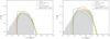 |
Fig. 6. Various fit of the reference numerical BSD (gray histogram) using power law parameterization from Sect. 3.1.1 (green lines) or logarithmic Softplus parameterization from Sect. 3.1.2 (orange lines) considering the dispersion (dashed lines) and not (solid lines). A numerical fit of the reference BSD using Eq. (1) from Furlanetto et al. (2004) inferring the efficiency parameter ζ is shown as a comparison (yellow dashed line). The fit is done at xH II ∼ 1% (left panel) and xH II ∼ 3% (right panel). |
In Fig. 7, we show the inferred Mcoll(Vion) relation with (dashed lines) and without (solid lines) including the dispersion for both our power law (green lines) and our logarithmic Softplus (orange lines) parameterizations. The cases with dispersion highlight the fact that the inference capability of our model strongly depends on the choice of an adequate functional form.
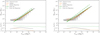 |
Fig. 7. Collapsed mass inside an ionized region as a function of its volume. The gray colormap represents the distribution of halos the HIRRAH-21 simulation and its numerical mean and dispersion are shown as black lines in the corresponding panels. The inferred relations with (dashed lines) and without (solid lines) considering the dispersion are shown for both our power law (green lines) and our logarithmic Softplus (orange lines) parameterizations. The fit is done at xH II ∼ 1% (left panel) and xH II ∼ 3% (right panel). |
Here, the simple power law model being less flexible and unreasonable for volumes where the mass resolution effect is dominant (V ≲ 2 cMpc3), the resulting theoretical BSD is unable to match the numerical BSD. To approach the numerical BSD as closely as possible, within the constraints of this functional form, the best-fit model overestimates the dispersion amplitude by a factor of ∼3. On the contrary, when using the logarithmic Softplus relation of Eq. (12), a functional form that is flexible enough to account for the mass resolution effect, the inferred mean Mcoll(Vion) relation is in very good agreement with the numerical one, though the dispersion seems to be somewhat underestimated in this case. In Table 1, we see that using the logarithmic Softplus relation in case of dispersion leads to a mean squared error of ≲0.1%, on the logarithm of the inferred physical relation Mcoll(Vion) for both xH II ∼ 1% and xH II ∼ 3%.
4.3. Model sensitivity to the halo mass formalism
The previous analysis was performed using the conditional mass function of Eq. (2), but (as stated in Sect. 2.4.1) our model can use various functional forms for the conditional mass functions that will logically affect the resulting BSD.
In Fig. 8, we represent the resulting BSD at xH II ∼ 1% for the same power law relation between the collapsed mass inside an ionized region and its volume using the CMF of Eq. (2) based on Sheth & Tormen (1999, green line) and the CMF of Eq. (3) based on Press & Schechter (1974, purple line). We observe an uniform decrease of the amplitude on the whole range for the CMF based on Press & Schechter (1974), compared to the one based on Sheth & Tormen (1999). The amplitude decrease can be explained by the fact that for a given volume, the regions that are ionized are most likely the ones with a large collapsed fraction. In Fig. 3, we show that the collapsed mass probability distribution peak is shifted to lower collapsed mass for Press & Schechter (1974) compared to Sheth & Tormen (1999). Therefore, a given volume is less likely to have a high collapsed mass for the former than for the latter, which consequently leads to an overall lower occurrence of bubbles in the Press & Schechter (1974) case for the same physical relation.
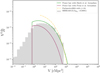 |
Fig. 8. Bubble size distribution at xH II ∼ 1% using the same parameters (inferred with the model using Sheth & Tormen 1999) in Eq. (11) using the CMF of Eq. (2) based on Sheth & Tormen (1999, green line) and the CMF of Eq. (3) based on Press & Schechter (1974, purple line). The Numerical BSD from the HIRRAH-21 simulation and a numerical fit of the reference BSD using Eq. (1) from Furlanetto et al. (2004) inferring the efficiency parameter ζ (yellow line) are shown for comparison. |
It is worth noting that the previous result is not a comparison of the quality of the inference between the two CMFs. Indeed the parameter values for the physical relation Mcoll(Vion) are those from the best fit using the CMF of Sheth & Tormen (1999). The theoretical BSD using Sheth & Tormen (1999) has thus been fitted to match the numerical BSD while the BSD using Press & Schechter (1974) CMF has not. This comparison strongly emphasizes the fact that the choice of mass function formalism has an effect which is non-negligible.
5. Extending the model in the percolation regime
In the previous section, we show that given an adequate functional form, the inference capability of our model is especially high when considering dispersion. However, even using dispersion, the inference power, and even the BSD matching capability of our model is strongly degraded for xH II > 10%. This effectively limits its inference possibilities to the early stages of the reionization process. The degradation is mainly due to the well-known percolation process (Furlanetto & Oh 2016), which has to be implemented in our model.
5.1. Implementing the percolation effect
To account for the percolation process without extensively modifying our model, we implement an algorithm that empirically emulates the effect of percolation on a distribution of bubbles where the possibility of overlap has been ignored. It thus takes as an input the BSD  for our model. The algorithm acts on each bin of volume, Vi, starting from the lowest and proceeds as follows :
First, we assume random, uncorrelated locations for bubble centers. If the center of a bubble of a given volume Vj > Vi is closer than Ri + Rj (where Rx is the radius corresponding to Vx) to the center of a bubble of volume, Vi, they are overlapping. There is therefore a shell around each bubble of volume Vj that generates an overlap. Considering all bubbles of size Vj, the total volume (per unit of volume) where an overlap with a bubble of size Vi can happen is calculated as:
![Mathematical equation: $$ \begin{aligned}V_{\text{ over}}^{i|j}= f_{\rm f}\left[\frac{4\pi }{3}(R_{i}+R_{j})^{3} - V_{j} \right] \mathrm{d}n_{\rm b}(V_{j}),\end{aligned} $$](/articles/aa/full_html/2022/11/aa44108-22/aa44108-22-eq41.gif)
where dnb(Vj) is the comoving number density of bubbles of volume, Vj, and ff is an empirical fudge factor. This fudge factor is needed to roughly account for the fact that ionized bubbles, such as the sources of ionizing photons, actually tend to be clustered and not homogeneously distributed.
Then, the number of bubbles of volume Vi, per unit volume, whose center falls in this overlapping zone (assuming uncorrelated center positions) is:
 (15)
(15)
Assuming that each percolation only involves one bubble of volume Vi and one of volume Vj,  is the number of bubbles in the two volumes bin that will percolate with a bubble of the other bin. There are
  bubbles of volume Vi and of volume Vj that percolate, thus the comoving number density of ionized bubbles in these two volumes bins is decreased accordingly:
We go on to approximate the volume of the bubbles that result from the percolation process as Vi + Vj – we note that this is obviously the value in the case where the two bubbles are just touching, the actual average value should be somewhat smaller, but also depends on the relative values of Vi and Vj. The comoving number density of ionized bubbles at this volume is thus increased by:

When all volume bins, Vj, have been considered for a given volume, Vi, the algorithm selects the next bin (in increasing volume order) and repeats the previous steps.
5.2. Results at xH II ≳ 10%
To assess the validity of our percolation algorithm, we fit the BSD at xH II ≳ 10%, where the percolation effect is dominant. Without prior knowledge on the value of the fudge factor, ff, we consider it as a free parameter to be fitted. In this regime, where the percolation is non-negligible, ionized bubbles more voluminous than a given volume have virtually all percolated into a single percolated cluster that spans the whole Universe, the remaining bubble growing inside neutral patches embedded into this percolated cluster. A sharp cut-off is therefore expected at large volume, creating a discontinuity in the BSD and making the fitting process tricky. We decided not to include the percolated cluster in the fit, as its volume depends on the simulation box size in the numerical simulation whereas it tends to infinity in our theoretical percolation algorithm. Additionally, if our fitted model happens to have a sharp cutoff at large volumes shifted by even only one bin compared to the numerical BSD cutoff, the resulting difference between the two BSDs in this bin will dramatically increase the value of the mean squared error, possibly disfavoring a set of parameter values that might have well reproduced the numerical BSD for all the other bins.
To tackle both issues, we perform the fit using the mean squared error computed on max in the interval 5 × 10⁻¹ cMpc3 ≲ V ≲ 106 cMpc3. We studied multiple other values of the 10−5 threshold and concluded that it does not change the parameter inference result significantly – only the absolute value of the error.
In Fig. 9, we show the fit of the reference numerical BSD (gray histogram) at xH II ∼ 10% (top) and xH II ∼ 22% (bottom) using the logarithmic Softplus parameterization, considering the dispersion with percolation (purple line) and without percolation (orange line). When using our percolation algorithm, the resulting BSD shape is closer to the numerical one and allows for a better fitting, especially of the sharp cut-off at high volumes. In Table 2, we show the mean squared relative error of the BSD fitting process computed with the adaptations explained above, for the logarithmic Softplus parameterization using dispersion with and without using the percolation algorithm at various global ionization fraction. We can see that in both cases, the mean squared error is always below 0.25 for xH II > 10% and it is divided by a factor of ∼2 when using percolation.
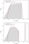 |
Fig. 9. Fit of the reference numerical BSD (gray histogram) at xH II ∼ 10% (top) and xH II ∼ 22% (bottom), using the logarithmic Softplus parameterization from Sect. 3.1.2 and considering the dispersion with percolation (purple line) and without percolation (orange line). |
Mean squared error computed on ![Mathematical equation: $ \log_{10}\left[\text{ max}\left( V^{2}\frac{\mathrm{d}n_{\mathrm{b}}}{\mathrm{d}V},10^{-5}\right)\right] $](/articles/aa/full_html/2022/11/aa44108-22/aa44108-22-eq48.gif) for 5 × 10⁻¹ ≲ V ≲ 106 for the logarithmic Softplus parameterization using dispersion with and without the use of the percolation algorithm at various global ionization fractions (xH II ∼ 10%, 16%, 22%, 30%, 38%, and 50%).
for 5 × 10⁻¹ ≲ V ≲ 106 for the logarithmic Softplus parameterization using dispersion with and without the use of the percolation algorithm at various global ionization fractions (xH II ∼ 10%, 16%, 22%, 30%, 38%, and 50%).
This decrease in the mean squared error when fitting the BSD comes with a better parameter prediction ability, compared to the case without percolation. In Fig. 10, we show the collapsed mass inside an ionized region as a function of its volume at at xH II ∼ 10% (top) and xH II ∼ 22% (bottom). The gray colormap represents the distribution of halos the HIRRAH-21 simulation and its numerical mean and dispersion are shown as black lines in the corresponding panels. We also show the inferred relations using the logarithmic Softplus parameterization considering the dispersion with percolation (purple line) and without percolation (orange line). We see that both the inferred relation Mcoll(Vion) and its dispersion are significantly closer to the numerical ones when using percolation. To quantify this improvement, in Table 3, we present the mean squared error of the physical Mcoll(Vion) relation reconstruction at various xH II. We see that the error on the inferred Mcoll(Vion) relation in the case with percolation is lower by an order of magnitude for xH II ≲ 30% and by a factor ∼5 for 30% ≲ xH II ≲ 50%, compared to the error in the case without percolation.
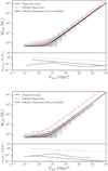 |
Fig. 10. Collapsed mass inside an ionized region as a function of its volume. The gray colormap represents the distribution of halos the HIRRAH-21 simulation and its numerical mean and dispersion are shown as black lines in the corresponding panels. The inferred relations using the logarithmic Softplus parameterization from Sect. 3.1.2 considering the dispersion with percolation (purple line) and without percolation (orange line) are shown. The fit is done at xH II ∼ 10% (top) and xH II ∼ 22% (bottom). |
Mean squared error of the physical Mcoll(Vion) relation reconstruction for the logarithmic Softplus parameterization using dispersion with and without using the percolation algorithm at various global ionization fraction (xH II ∼ 10%, 16%, 22%, 30%, 38%, and 50%).
However, in Fig. 10 and Table 3, we also see that the mean squared error is increasing with increasing xH II. This is not surprising as, for example, for large average ionization fractions, the percolation increasingly involve the non-spherical percolated cluster, deviating from the simple sphere overlap considered in our model. Nonetheless, until xH II ∼ 30% our percolation algorithm still allows us to infer the physical Mcoll(Vion) relation with an mean squared error lower than 15%.
In Fig. 11, we represent the evolution of the fudge factor (resulting from the fitting process) as a function of the global ionization fraction xH II. It appears to increase more or less linearly on the studied range of 0.10 ≲ xH II ≲ 0.50. One motivation for introducing this fudge factor is to correct for the fact that the positions of the ionized bubbles are in reality not uncorrelated, as is assumed in our simple percolation model. Thus, it is not surprising that we need higher values in situations where bubble overlap is more present. Another contribution to the fudge factor may be the departure from the assumed spherical geometry, which is also getting stronger as the percolation process progresses.
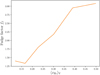 |
Fig. 11. Evolution of the fudge factor, ff, as a function of the volume-weighted global ionization fraction, ⟨xH II⟩V. |
6. Conclusions
In this work, we develop a new analytical model to compute the ionized bubble size distribution of the Epoch of Reionization (5 ≲ z ≲ 15) starting from the underlying physical relation between the collapsed mass inside an ionized region and its size. We compare it to both the fiducial model of Furlanetto et al. (2004) and the numerical results from the HIRRAH-21 simulation for global ionization fractions of xH II ∼ 1%,3%,10%,16%,22%,30%,38%, and 50%. The HIRRAH-21 simulation is composed of 20483 particles in a 200 h−1 cMpc box and was performed using the LICORICE code, which fully couples the hydrodynamics with the radiative transfer of ionizing UV and X-rays. The key features and results of our models are as follows:
-
The underlying physical relation between the collapsed mass inside an ionized region and its volume is totally parameterizable, whereas in the original model by Furlanetto et al. (2004) it takes a fixed form that enables an analytical computation. In our model, it is possible to use any functional form and obtain the resulting BSD. In this study, we use two functional forms: a power law and a logarithmic softplus, both producing a BSD in strong agreement with the numerical BSD directly computed from the HIRRAH-21 simulation before the percolation regime at xH II ≲ 10%.
-
More than just the functional form, our model is largely adaptable to different theoretical frameworks. As it is based on the halo conditional mass function theory, it can use various mass function formalisms such as Press & Schechter (1974) and Sheth & Tormen (1999) formalisms. It could even accommodate a numerically determined conditional mass function, so that no biases are introduced. One can choose to include the sample variance effect if needed. A functional form for the dispersion in the underlying Mcoll(Vion) physical relation can also be implemented.
-
Using various algorithms, our model can infer the Mcoll(Vion) relation from the observed BSD. Before the percolation regime, for our two choices of parameterization, the resulting physical relation is in accordance with the relation computed from the HIRRAH-21 simulation, thus demonstrating the inference capability of the model. Further studies using results from other simulation codes would be useful to better assess this inference capability.
-
We also developed a percolation algorithm that can apply a percolation effect to an existing BSD computed without percolation. Good performances rely on introducing a fudge factor whose optimal value seems to be dependent on the average ionization fraction, although with a simple linear relation across the studied range. Using this algorithm, our model keeps a strong inference capability even in the percolation regime as it can recover the physical relation with a mean squared error lower than 1% for xH II ≲ 16% and lower than 15% for xH II ≲ 30% for the softplus parameterization. The inference capability decreases with increasing global ionization as it is likely that the underlying approximations of our percolation algorithm would not stand at the latest stage of percolation.
Let us emphasize again that the Mcoll(Vion) parameterization can be readily interpreted in term of underlying physical processes. For example, in the logarithmic softplus parameterization, Mcoll, th, is essentially the minimum halo mass for efficient star formation, especially if α ∼ 1, Vth was proportional to the amount of radiation emitted per unit collapsed mass. Thus, constraining Mcoll(Vion) really provides information on the astrophysics.
It is necessary to mention that the effect of thermal noise, imperfect calibration, and foreground removal and limited angular resolution will impact the quality of the tomographic data from which an observed BSD will be derived. The limited angular resolution of real observations will at least result in a cut-off of the BSD on small scales that will limit the range of scales that can be used in the inference process. It will also impact the general shape of the BSD on larger scales (Giri et al. 2018). It is possible that our model could be improved to include the effect of angular resolution with a similar approach (just as for the effect of percolation) but at this stage, this remains an open question. A variance in each bin of the observed BSD resulting from various sources, starting with the thermal noise, could be taken into account by using a χ2 evaluation for the goodness of fit.
A more difficult issue is the current domain of validity of the model (i.e., xH II ≲ 30% at best). This likely corresponds to redshifts z ≳ 9 while the signal-to-noise ratio of observations with radio interferometers such as SKA degrades with increasing redshift. One way to tackle this issue would be to devise a more sophisticated percolation model that would describe more precisely the spatial correlation in the ionized bubble distribution. Then, our BSD model would likely be valid at higher ionization fractions as well as at lower redshifts. In any case, the inferred parameters will then have posterior distributions with a potentially broad variance. Quantifying this aspect and making a comparison to the constraints that can be derived from other quantities such as the signal power spectrum will be necessary for future studies.
Acknowledgments
This work was performed using HPC resources from GENCI-CINES (grant 2018-A0050410557).
References
- Abdurashidova, Z., Aguirre, J. E., Alexander, P., et al. 2022, ApJ, 924, 51 [NASA ADS] [CrossRef] [Google Scholar]
- Asad, K. M., Koopmans, L. V., Jelic, V., et al. 2015, MNRAS, 451, 3709 [NASA ADS] [CrossRef] [Google Scholar]
- Baek, S., Di Matteo, P., Semelin, B., Combes, F., & Revaz, Y. 2009, A&A, 495, 389 [NASA ADS] [CrossRef] [EDP Sciences] [Google Scholar]
- Baek, S., Semelin, B., Di Matteo, P., Revaz, Y., & Combes, F. 2010, A&A, 523, A4 [NASA ADS] [CrossRef] [EDP Sciences] [Google Scholar]
- Barkana, R., & Loeb, A. 2004, ApJ, 609, 474 [NASA ADS] [CrossRef] [Google Scholar]
- Bernardi, G., De Bruyn, A. G., Brentjens, M. A., et al. 2009, A&A, 500, 965 [NASA ADS] [CrossRef] [EDP Sciences] [Google Scholar]
- Bernardi, G., de Bruyn, A. G., Harker, G., et al. 2010, A&A, 522, A67 [NASA ADS] [CrossRef] [EDP Sciences] [Google Scholar]
- Bevins, H. T. J., Handley, W. J., Fialkov, A., de Lera Acedo, E., & Javid, K. 2021, MNRAS, 508, 2923 [NASA ADS] [CrossRef] [Google Scholar]
- Bianco, M., Giri, S. K., Iliev, I. T., & Mellema, G. 2021, MNRAS, 505, 3982 [NASA ADS] [CrossRef] [Google Scholar]
- Bond, J. R., Cole, S., Efstathiou, G., & Kaiser, N. 1991, ApJ, 379, 440 [NASA ADS] [CrossRef] [Google Scholar]
- Bosman, S. E. I., Davies, F. B., Becker, G. D., et al. 2022, MNRAS, 514, 55 [NASA ADS] [CrossRef] [Google Scholar]
- Bye, C. H., Portillo, S. K. N., & Fialkov, A. 2022, ApJ, 930, 79 [NASA ADS] [CrossRef] [Google Scholar]
- Cohen, A., Fialkov, A., & Barkana, R. 2016, MNRAS, 459, L90 [NASA ADS] [CrossRef] [Google Scholar]
- Cohen, A., Fialkov, A., Barkana, R., & Monsalve, R. A. 2020, MNRAS, 495, 4845 [NASA ADS] [CrossRef] [Google Scholar]
- Davis, M., Efstathiou, G., Frenk, C. S., & White, S. D. M. 1985, ApJ, 292, 371 [Google Scholar]
- Doussot, A., Eames, E., & Semelin, B. 2019, MNRAS, 490, 371 [NASA ADS] [CrossRef] [Google Scholar]
- Fan, X., Strauss, M. A., Becker, R. H., et al. 2006, AJ, 132, 117 [NASA ADS] [CrossRef] [Google Scholar]
- Friedrich, M. M., Mellema, G., Alvarez, M. A., Shapiro, P. R., & Iliev, I. T. 2011, MNRAS, 413, 1353 [NASA ADS] [CrossRef] [Google Scholar]
- Furlanetto, S. R., & Oh, S. P. 2016, MNRAS, 457, 1813 [NASA ADS] [CrossRef] [Google Scholar]
- Furlanetto, S. R., Zaldarriaga, M., & Hernquist, L. 2004, ApJ, 613, 1 [NASA ADS] [CrossRef] [Google Scholar]
- Furlanetto, S. R., Oh, S. P., & Briggs, F. H., 2006, Phys. Rep., 433, 181 [Google Scholar]
- Gangolli, N., Aloisio, D. A., Nasir, F., & Zheng, Z. 2021, MNRAS, 501, 5294 [NASA ADS] [CrossRef] [Google Scholar]
- Ghara, R., Giri, S. K., Mellema, G., et al. 2020, MNRAS, 493, 4728 [NASA ADS] [CrossRef] [Google Scholar]
- Ghara, R., Giri, S. K., Ciardi, B., Mellema, G., & Zaroubi, S. 2021, MNRAS, 503, 4551 [NASA ADS] [CrossRef] [Google Scholar]
- Ghosh, A., Bharadwaj, S., Ali, S. S., & Chengalur, J. N. 2011, MNRAS, 418, 2584 [NASA ADS] [CrossRef] [Google Scholar]
- Gillet, N., Mesinger, A., Greig, B., Liu, A., & Ucci, G. 2019, MNRAS, 10, 1 [Google Scholar]
- Giri, S. K., Mellema, G., Dixon, K. L., & Iliev, I. T. 2018, MNRAS, 473, 2949 [NASA ADS] [CrossRef] [Google Scholar]
- Giri, S. K., Mellema, G., Aldheimer, T., Dixon, K. L., & Iliev, I. T. 2019, MNRAS, 489, 1590 [NASA ADS] [CrossRef] [Google Scholar]
- Greig, B., & Mesinger, A. 2015, MNRAS, 449, 4246 [NASA ADS] [CrossRef] [Google Scholar]
- Greig, B., & Mesinger, A. 2017, MNRAS, 472, 2651 [NASA ADS] [CrossRef] [Google Scholar]
- Greig, B., & Mesinger, A. 2018, MNRAS, 477, 3217 [NASA ADS] [CrossRef] [Google Scholar]
- Greig, B., Mesinger, A., Koopmans, L. V., et al. 2021a, MNRAS, 501, 1 [Google Scholar]
- Greig, B., Trott, C. M., Barry, N., et al. 2021b, MNRAS, 500, 5322 [Google Scholar]
- Hahn, O., & Abel, T. 2011, MNRAS, 415, 2101 [Google Scholar]
- Hassan, S., Andrianomena, S., & Doughty, C. 2020, MNRAS, 494, 5761 [NASA ADS] [CrossRef] [Google Scholar]
- Hortúa, H. J., Volpi, R., & Malagò, L. 2020, ArXiv e-prints [arXiv:2005.02299] [Google Scholar]
- Jelic, V., de Bruyn, A. G., Mevius, M., et al. 2014, A&A, 568, A101 [NASA ADS] [CrossRef] [EDP Sciences] [Google Scholar]
- Jennings, W. D., Watkinson, C. A., Abdalla, F. B., & McEwen, J. D. 2019, MNRAS, 483, 2907 [NASA ADS] [CrossRef] [Google Scholar]
- Kern, N. S., Liu, A., Parsons, A. R., Mesinger, A., & Greig, B. 2017, ApJ, 848, 23 [NASA ADS] [CrossRef] [Google Scholar]
- Koopmans, L., Pritchard, J., Mellema, G., et al. 2015, in Proceedings of Advancing Astrophysics with the Square Kilometre Array - PoS(AASKA14) (Trieste, Italy: Sissa Medialab), 9, 001 [NASA ADS] [Google Scholar]
- Lacey, C., & Cole, S. 1993, MNRAS, 262, 627 [NASA ADS] [CrossRef] [Google Scholar]
- Lacey, C., & Cole, S. 1994, MNRAS, 271, 676 [Google Scholar]
- Lin, Y., Oh, S. P., Furlanetto, S. R., & Sutter, P. M. 2016, MNRAS, 461, 3361 [NASA ADS] [CrossRef] [Google Scholar]
- Line, J. L., Webster, R. L., Pindor, B., Mitchell, D. A., & Trott, C. M. 2017, PASA, 34, 003 [NASA ADS] [CrossRef] [Google Scholar]
- List, F., & Lewis, G. F. 2020, MNRAS, 493, 5913 [NASA ADS] [CrossRef] [Google Scholar]
- McGreer, I. D., Mesinger, A., & D’Odorico, V. 2015, MNRAS, 447, 499 [NASA ADS] [CrossRef] [Google Scholar]
- Mellema, G., Koopmans, L. V. E., Abdalla, F. A., et al. 2013, Exp. Astron., 36, 235 [NASA ADS] [CrossRef] [Google Scholar]
- Mesinger, A., & Furlanetto, S. 2007, ApJ, 669, 663 [Google Scholar]
- Mesinger, A., Furlanetto, S., & Cen, R. 2011, MNRAS, 411, 955 [Google Scholar]
- Mondal, R., Fialkov, A., Fling, C., et al. 2020, MNRAS, 498, 4178 [NASA ADS] [CrossRef] [Google Scholar]
- Monsalve, R. A., Fialkov, A., Bowman, J. D., et al. 2019, ApJ, 875, 67 [NASA ADS] [CrossRef] [Google Scholar]
- Murray, S., Power, C., & Robotham, A. 2013, Astron. Comput., 3, 23 [CrossRef] [Google Scholar]
- Murray, S., Diemer, B., Chen, Z., et al. 2021, Astron. Comput., 36, 100487 [NASA ADS] [CrossRef] [Google Scholar]
- Naoz, S., Noter, S., & Barkana, R. 2006, MNRAS, 373, 98 [Google Scholar]
- Offringa, A. R., Trott, C. M., Hurley-Walker, N., et al. 2016, MNRAS, 458, 1057 [Google Scholar]
- Paranjape, A., & Choudhury, T. R. 2014, MNRAS, 442, 1470 [NASA ADS] [CrossRef] [Google Scholar]
- Paranjape, A., Choudhury, T. R., & Padmanabhan, H. 2016, MNRAS, 460, 1801 [NASA ADS] [CrossRef] [Google Scholar]
- Planck Collaboration XIII. 2016, A&A, 594, A13 [NASA ADS] [CrossRef] [EDP Sciences] [Google Scholar]
- Pober, J. C., Liu, A., Dillon, J. S., et al. 2014, ApJ, 782, 66 [NASA ADS] [CrossRef] [Google Scholar]
- Prelogović, D., Mesinger, A., Murray, S., Fiameni, G., & Gillet, N. 2021, MNRAS, 509, 3852 [CrossRef] [Google Scholar]
- Press, W. H., & Schechter, P. 1974, ApJ, 187, 425 [Google Scholar]
- Procopio, P., Wayth, R. B., Line, J., et al. 2017, PASA, 34, e033 [NASA ADS] [CrossRef] [Google Scholar]
- Qin, Y., Mesinger, A., Bosman, S. E. I., & Viel, M. 2021, MNRAS, 506, 2390 [NASA ADS] [CrossRef] [Google Scholar]
- Remazeilles, M., Dickinson, C., Banday, A. J., Bigot-Sazy, M. A., & Ghosh, T. 2015, MNRAS, 451, 4311 [NASA ADS] [CrossRef] [Google Scholar]
- Rubiño-Martín, J. A., Betancort-Rijo, J., & Patiri, S. G. 2008, MNRAS, 386, 2181 [CrossRef] [Google Scholar]
- Schmit, C. J., & Pritchard, J. R. 2018, MNRAS, 475, 1213 [NASA ADS] [CrossRef] [Google Scholar]
- Semelin, B. 2016, MNRAS, 455, 962 [NASA ADS] [CrossRef] [Google Scholar]
- Semelin, B., & Combes, F. 2002, A&A, 388, 826 [NASA ADS] [CrossRef] [EDP Sciences] [Google Scholar]
- Semelin, B., Eames, E., Bolgar, F., & Caillat, M. 2017, MNRAS, 472, 4508 [NASA ADS] [CrossRef] [Google Scholar]
- Sheth, R. K., & Tormen, G. 1999, MNRAS, 308, 119 [Google Scholar]
- Sheth, R. K., Mo, H. J., & Tormen, G. 2001, MNRAS, 323, 1 [NASA ADS] [CrossRef] [Google Scholar]
- Shimabukuro, H., & Semelin, B. 2017, MNRAS, 468, 3869 [NASA ADS] [CrossRef] [Google Scholar]
- Yatawatta, S., de Bruyn, A. G., Brentjens, M. A., et al. 2013, A&A, 550, A136 [NASA ADS] [CrossRef] [EDP Sciences] [Google Scholar]
- Zahn, O., Lidz, A., McQuinn, M., et al. 2007, ApJ, 654, 12 [NASA ADS] [CrossRef] [Google Scholar]
- Zhao, X., Mao, Y., Cheng, C., & Wandelt, B. D. 2022a, ApJ, 926, 151 [NASA ADS] [CrossRef] [Google Scholar]
- Zhao, X., Mao, Y., & Wandelt, B. D. 2022b, ApJ, 933, 236 [NASA ADS] [CrossRef] [Google Scholar]
All Tables
Mean squared error computed on for 5 × 10⁻¹ ≲ V ≲ 106 for the logarithmic Softplus parameterization using dispersion with and without the use of the percolation algorithm at various global ionization fractions (xH II ∼ 10%, 16%, 22%, 30%, 38%, and 50%).
Mean squared error of the physical Mcoll(Vion) relation reconstruction for the logarithmic Softplus parameterization using dispersion with and without using the percolation algorithm at various global ionization fraction (xH II ∼ 10%, 16%, 22%, 30%, 38%, and 50%).
All Figures
|
Fig. 1. Volume-weighted ionized (purple) and neutral (orange) fraction as a function of the redshift from the HIRRAH-21 simulation. |
| In the text | |
|
Fig. 2. Bubble size distribution from the HIRRAH-21 simulation at global ionization fractions xH II ∼ 1%, 3%, 10%, and 20% for ionization thresholds, |
| In the text | |
|
Fig. 3. Collapsed mass distribution computed at redshift z ∼ 9.8 (corresponding to xH II ∼ 1%) considering the sample variance (dashed lines) or not (solid lines) using the conditional mass function of Eq. (3) (purple) or of Eq. (2) (yellow). The results are shown for ionized regions of radius of: 0.4 cMpc, 3 cMpc, 10 cMpc, and 20 cMpc. |
| In the text | |
|
Fig. 4. Various fit of the reference numerical BSD (gray histogram) using a power law parameterization from Sect. 3.1.1 (green lines) or a logarithmic Softplus parameterization from Sect. 3.1.2 (orange lines) considering the sample variance (dashed lines) or otherwise (solid lines). A numerical fit of the reference BSD from Furlanetto et al. (2004; Eq. (1)) using only the efficiency parameter ζ is shown as a comparison (yellow dashed line). The fit is done at xH II ∼ 1% (left panel) and xH II ∼ 3% (right panel). |
| In the text | |
|
Fig. 5. Collapsed mass inside an ionized region as a function of its volume. The gray colormap represents the distribution of halos the HIRRAH-21 simulation and its numerical mean (top panel) and dispersion (bottom panel) are shown as black lines in the corresponding panels. The inferred relations with (dashed lines) and without (solid lines) considering the sample variance are shown for both our power law (green lines) and our logarithmic Softplus (orange lines) parameterizations. The fit is done at xH II ∼ 1% (left panel) and xH II ∼ 3% (right panel). |
| In the text | |
|
Fig. 6. Various fit of the reference numerical BSD (gray histogram) using power law parameterization from Sect. 3.1.1 (green lines) or logarithmic Softplus parameterization from Sect. 3.1.2 (orange lines) considering the dispersion (dashed lines) and not (solid lines). A numerical fit of the reference BSD using Eq. (1) from Furlanetto et al. (2004) inferring the efficiency parameter ζ is shown as a comparison (yellow dashed line). The fit is done at xH II ∼ 1% (left panel) and xH II ∼ 3% (right panel). |
| In the text | |
|
Fig. 7. Collapsed mass inside an ionized region as a function of its volume. The gray colormap represents the distribution of halos the HIRRAH-21 simulation and its numerical mean and dispersion are shown as black lines in the corresponding panels. The inferred relations with (dashed lines) and without (solid lines) considering the dispersion are shown for both our power law (green lines) and our logarithmic Softplus (orange lines) parameterizations. The fit is done at xH II ∼ 1% (left panel) and xH II ∼ 3% (right panel). |
| In the text | |
|
Fig. 8. Bubble size distribution at xH II ∼ 1% using the same parameters (inferred with the model using Sheth & Tormen 1999) in Eq. (11) using the CMF of Eq. (2) based on Sheth & Tormen (1999, green line) and the CMF of Eq. (3) based on Press & Schechter (1974, purple line). The Numerical BSD from the HIRRAH-21 simulation and a numerical fit of the reference BSD using Eq. (1) from Furlanetto et al. (2004) inferring the efficiency parameter ζ (yellow line) are shown for comparison. |
| In the text | |
|
Fig. 9. Fit of the reference numerical BSD (gray histogram) at xH II ∼ 10% (top) and xH II ∼ 22% (bottom), using the logarithmic Softplus parameterization from Sect. 3.1.2 and considering the dispersion with percolation (purple line) and without percolation (orange line). |
| In the text | |
|
Fig. 10. Collapsed mass inside an ionized region as a function of its volume. The gray colormap represents the distribution of halos the HIRRAH-21 simulation and its numerical mean and dispersion are shown as black lines in the corresponding panels. The inferred relations using the logarithmic Softplus parameterization from Sect. 3.1.2 considering the dispersion with percolation (purple line) and without percolation (orange line) are shown. The fit is done at xH II ∼ 10% (top) and xH II ∼ 22% (bottom). |
| In the text | |
|
Fig. 11. Evolution of the fudge factor, ff, as a function of the volume-weighted global ionization fraction, ⟨xH II⟩V. |
| In the text | |
Current usage metrics show cumulative count of Article Views (full-text article views including HTML views, PDF and ePub downloads, according to the available data) and Abstracts Views on Vision4Press platform.
Data correspond to usage on the plateform after 2015. The current usage metrics is available 48-96 hours after online publication and is updated daily on week days.
Initial download of the metrics may take a while.