| Issue |
A&A
Volume 663, July 2022
|
|
|---|---|---|
| Article Number | A126 | |
| Number of page(s) | 11 | |
| Section | Galactic structure, stellar clusters and populations | |
| DOI | https://doi.org/10.1051/0004-6361/202243195 | |
| Published online | 19 July 2022 | |
Galactic ArchaeoLogIcaL ExcavatiOns (GALILEO)
I. An updated census of APOGEE N-rich giants across the Milky Way⋆
1
Instituto de Astronomía, Universidad Católica del Norte, Av. Angamos 0610, Antofagasta, Chile
e-mail: jose.fernandez@ucn.cl
2
Department of Physics and JINA Center for the Evolution of the Elements, University of Notre Dame, Notre Dame, IN, 46556, USA
3
Universidade de São Paulo, IAG, Rua do Matão 1226, Cidade Universitária, São Paulo, 05508-900, Brazil
4
Depto. de Cs. Físicas, Facultad de Ciencias Exactas, Universidad Andrés Bello, Av. Fernández Concha 700, Las Condes, Santiago, Chile
5
Vatican Observatory, 00120 Vatican City State, Italy
6
Leibniz-Institut für Astrophysik Potsdam (AIP), An der Sternwarte 16, 14482 Potsdam, Germany
7
Laboratório Interinstitucional de e-Astronomia – LIneA, Rua Gal. José Cristino 77, Rio de Janeiro, RJ 20921-400, Brazil
8
School of Physics and Astronomy, Sun Yat-sen University, Zhuhai 519082, China
9
ExtraUniversidade Federal do Rio Grande do Sul, Instituto de Física, Av. Bento Gonçalves 9500, Porto Alegre, RS, Brazil
10
Departamento de Astronomía, Universidad de Concepción, Casilla 160-C, Concepción, Chile
11
Department of Astronomy – Universidad de La Serena, Av. Juan Cisternas, 1200 North, La Serena, Chile
12
Instituto de Investigación Multidisciplinario en Ciencia y Tecnología, Universidad de La Serena, Benavente 980, La Serena, Chile
13
Centro de Investigación en Astronomía, Universidad Bernardo O’Higgins, Avenida Viel 1497, Santiago, Chile
Received:
25
January
2022
Accepted:
30
March
2022
We use the 17th data release of the second phase of the Apache Point Observatory Galactic Evolution Experiment (APOGEE-2) to provide a homogenous census of N-rich red giant stars across the Milky Way (MW). We report a total of 149 newly identified N-rich field giants toward the bulge, metal-poor disk, and halo of our Galaxy. They exhibit significant enrichment in their nitrogen abundance ratios ([N/Fe] ≳ +0.5), along with simultaneous depletions in their [C/Fe] abundance ratios ([C/Fe] < +0.15), and they cover a wide range of metallicities (−1.8 < [Fe/H] < −0.7). The final sample of candidate N-rich red giant stars with globular-cluster-like (GC-like) abundance patterns from the APOGEE survey includes a grand total of ∼412 unique objects. These strongly N-enhanced stars are speculated to have been stripped from GCs based on their chemical similarities with these systems. Even though we have not found any strong evidence for binary companions or signatures of pulsating variability yet, we cannot rule out the possibility that some of these objects were members of binary systems in the past and/or are currently part of a variable system. In particular, the fact that we identify such stars among the field stars in our Galaxy provides strong evidence that the nucleosynthetic process(es) producing the anomalous [N/Fe] abundance ratios occurs over a wide range of metallicities. This may provide evidence either for or against the uniqueness of the progenitor stars to GCs and/or the existence of chemical anomalies associated with likely tidally shredded clusters in massive dwarf galaxies such as “Kraken/Koala”, Gaia-Enceladus-Sausage, among others, before or during their accretion by the MW. A dynamical analysis reveals that the newly identified N-rich stars exhibit a wide range of dynamical characteristics throughout the MW, indicating that they were produced in a variety of Galactic environments.
Key words: stars: abundances / techniques: spectroscopic / globular clusters: general / stars: chemically peculiar
Full Tables 1 and 3 are only available at the CDS via anonymous ftp to cdsarc.u-strasbg.fr (130.79.128.5) or via http://cdsarc.u-strasbg.fr/viz-bin/cat/J/A+A/663/A126
© ESO 2022
1. Introduction
The formation and assembly history of the Milky Way (MW) reveal that during early epochs it was an inexhaustible galactic cannibal, which has completely devoured a number of other large and massive dwarf galaxies some 9–11 Gyr ago (see e.g., Kruijssen et al. 2020; Helmi 2020). Some of these now defunct dwarf galaxies have been identified as stellar structures or debris that populate the present-day Galactic field (e.g., the bulge, disk, and/or halo of the MW), and they are very phase mixed. Among the most populated progenitors associated to these systems are the Helmi Stream (Helmi et al. 1999; Chiba & Beers 2000), the Gaia-Sausage (Belokurov et al. 2018) also referred to as Gaia-Enceladus (Helmi et al. 2018), Sequoia (Myeong et al. 2019; Barbá et al. 2019), Thamnos (Koppelman et al. 2019), Kraken/Koala (Kruijssen et al. 2020; Forbes 2020), and Pontus (Malhan et al. 2022), which serve as the fossil records of the events that created them, acting as time capsules that preserve the dynamical and chemical memory of the MW assembly history.
Besides the ancient accretion events, there is a wealth of observational evidence for a more recent (< 7 Gyr ago; see e.g., Kruijssen et al. 2020) event which corresponds to the Sagittarius dwarf spheroidal galaxy (Ibata et al. 1994; Hasselquist et al. 2017, 2019) and its dispersed streams (Hasselquist et al. 2017, 2019), which also preserve traces of tidal stripping and disruption of globular clusters (GCs; see e.g., Fernández-Trincado et al. 2021c), followed by the unusual Omega Centauri (NGC 5139) system (Villanova et al. 2014), together with its hypothesized “Fimbulthul” stream (Ibata et al. 2019) as well as its controversial tidal tails and stellar debris (Da Costa & Coleman 2008; Majewski et al. 2012; Fernández-Trincado et al. 2015a,b; Marconi et al. 2014; Sollima 2020), and a number of stellar streams with variate origins and over a wide range of metallicities (Wan et al. 2020; Martin et al. 2022). These claims are bolstered by the detection of extratidal stars with unusual GC-like abundance patterns, similar to that seen toward the Large and Small Magellanic systems today (Fernández-Trincado et al. 2020b), the stellar halo (Hanke et al. 2020), and the Galactic bulge (Minniti et al. 2018; Fernández-Trincado et al. 2021b).
In addition to the major accretion events, the Galactic field is also polluted by a plethora of minor substructures (Koppelman et al. 2019), some of which have been named Aleph, Arjuna, I’itoi, LMS-1 (Wukong), among other (see e.g., Naidu et al. 2020; Malhan et al. 2022). These substructures are in turn accompanied by a number of chemically atypical stars associated with dissolved GCs, such as the genuine population of giants with GC second-generation-like chemical patterns (Fernández-Trincado et al. 2016a, 2017) identified toward the bulge, disk, and inner halo (Fernández-Trincado et al. 2020d). The recently discovered “Jurassic” substructure (Fernández-Trincado et al. 2019a, 2020a) is accompanied by a prominent population of aluminum-enhanced stars buried in the inner Galaxy (Fernández-Trincado et al. 2020c; Lucey et al. 2022). There is also a recently discovered population of high-metallicity ([Fe/H] > −0.7) giants with atmospheres strongly enhanced in nitrogen and aluminum (Fernández-Trincado et al. 2021d) well above typical Galactic levels.
All of these chemically unusual populations were likely formed after the infall of major satellites and/or stellar clusters during different epochs of MW evolution, as envisioned by many studies (see e.g., Leon et al. 2000; Majewski et al. 2012; Kunder et al. 2014; Anguiano et al. 2015; Fernández-Trincado et al. 2015a,b, 2016a,b; Lind et al. 2015; Recio-Blanco et al. 2017; Minniti et al. 2018; Kundu et al. 2019a,b, 2021; Hanke et al. 2020; Sollima 2020 and references therein). Based on low- and high-resolution spectroscopic surveys, several pioneering works have searched for traces of a unique and exclusive collection of field stars that contrast with the typical chemical composition of the majority of Galactic stars, and they are uniquely distinctive in some of the canonical abundance planes and speculated to belong to the population of GCs’ escapee. Among these field stars are the nitrogen-enhanced metal-poor stars (NEMP; Johnson et al. 2007) with [C/N] < −0.5 and [N/Fe] > +0.5, which have also been exclusively identified in GC environments (see e.g., Simpson & Martell 2019).
Previous studies along these lines include a unique collection of carbon-deficient ([C/Fe]< + 0.15) nitrogen-enhanced field stars (hereafter N-rich stars) identified toward the inner Galaxy by Fernández-Trincado et al. (2016a) and Martell et al. (2016); toward the bulge field by Schiavon et al. (2017) and Fernández-Trincado et al. (2017, 2019b); and an extra-tidal N-rich star from the bulge GC NGC 6723 was identified by Fernández-Trincado et al. (2021b). A number of more recently added examples are from Kisku et al. (2021) in the inner Galaxy, toward the disk field, and beyond the tidal radius of Palomar 5 by Fernández-Trincado et al. (2019b), and in the field of the Large and Small Magellanic Clouds (LMC and SMC, respectively) and the Sagittarius Spheroidal galaxy by Fernández-Trincado et al. (2020b, 2021c), respectively. Additionally, the similarity in orbital properties between GCs and N-rich field stars (or previously called “CN-strong field stars”) was demonstrated in Carollo et al. (2013) and Tang et al. (2020). While the wide gamut of elemental abundances recently examined by Yu et al. (2021) with optical spectra for some of these N-rich stars strengthened their exclusive link to GCs.
Besides the carbon-deficient N-rich field stars, there is a significant population of carbon-deficient aluminum-enriched field stars (hereafter Al-rich stars) that exhibit low and high levels of nitrogen abundance ratios (Fernández-Trincado et al. 2020c), suggesting that there are at least two groups of N-rich field stars that have likely been formed from two different nucleosynthetic pathways over a wide range of metallicities. Such anomalous abundance patterns are found in many GCs over a wide range of metallicities (Fernández-Trincado et al. 2019d, 2020e, 2021a; Fernández-Trincado et al. 2022a,b; Mészáros et al. 2020, 2021; Geisler et al. 2021; Romero-Colmenares et al. 2021; Masseron et al. 2019), and even into the most metal-poor MW GC (see e.g., Fernández-Trincado et al. 2021e). Thus, the escape of stars from GCs could be a plausible explanation for the presence of these chemically anomalous stars in the Galactic field.
Although the recognized number of such chemically anomalous field stars has expanded greatly during the last decades, the origin of their unusual abundance signatures remains under discussion. For instance, recently, Bekki (2019) proposed an alternative way to produce these N-rich stars, which could be formed in high-density environments. More recently, Fernández-Trincado et al. (2019c) has confirmed the existence of a N-rich star in a genuine binary system, which owes its nitrogen enrichment to binary mass transfer of an evolved asymptotic giant branch (AGB) star that is likely now a white dwarf. There still remains the possibility that a high fraction of the N-rich and Al-rich field stars could be evolved objects, possibly an “early-AGB” or an AGB star, rather than being formed through GC self-enrichment (see e.g., Pereira et al. 2017). The presence of such a young and moderately metal-poor star in the Galactic field would have important implications. However, its nature remains uncertain.
As emphasized by Tang et al. (2019), some of the CH-normal field stars and the N-rich field stars could have a very similar origin, and likely they share the same nucleosynthetic pathways. The wide range of elemental abundances recently examined by Yu et al. (2021) for some of these N-rich stars has strengthened the proposed link to GCs. Thus, future dedicated long-term radial-velocity monitoring of all of these stars would naturally be the best course of action in order to offer clues about the rare astrophysical events behind these unique and atypical objects in the MW.
The zoo of chemically anomalous stars in the Galactic field is very diverse. In addition to the previously mentioned N-rich and Al-rich stars, substantial evidence has been offered for the existence of Si-rich stars (Fernández-Trincado et al. 2019a, 2020a), K-rich stars (Kemp et al. 2018), r-process enriched stars (Holmbeck et al. 2020; Gudin et al. 2021; Shank et al. 2022), s-process enriched stars (Anders et al. 2018; Pereira et al. 2019a), Na-rich stars (Pereira et al. 2019b; Koo et al. 2022), and P-rich stars (Masseron et al. 2020a,b) over a wide range of metallicities, and they are thought to form through different nucleosynthetic channels.
Here, we report the results of the analysis of the final and complete data release of the Apache Point Observatory Galactic Evolution Experiment II survey (APOGEE-2; Majewski et al. 2017) through Galactic ArchaeoLogIcaL ExcavatiOns (GALILEO). This project dedicated to searching for and detecting chemically anomalous giants – including the stars that show anomalously high levels of [N/Fe] and [Al/Fe] – for long-term radial-velocity monitoring to better understand the nature of these stars with unusual elemental abundances, as well as its nucleosynthetic pathways.
2. Observations and data
We employed high-resolution (R ∼ 22 500) near-infrared (NIR) spectra taken from the final APOGEE-2 seventeenth data release (DR 17; Abdurro’uf et al. 2022), which is one of the internal programs of the Sloan Digital Sky Survey-IV (Blanton et al. 2017). These programs have been developed to provide precise radial velocities (RVs) < 1 km s−1 and elemental abundances for over 700 000 unique stars across the MW and nearby systems.
APOGEE-2 observations were carried out through two identical spectrographs (Wilson et al. 2019) from the Northern Hemisphere on the 2.5m telescope at Apache Point Observatory (APO, APOGEE-2N; Gunn et al. 2006) and from the Southern Hemisphere on the Irénée du Pont 2.5m telescope (Bowen & Vaughan 1973) at Las Campanas Observatory (LCO, APOGEE-2S). Each instrument records most of the H band (1.51 μm–1.69 μm) on three detectors, with coverage gaps between ∼1.58–1.59 μm and ∼1.64–1.65 μm, and with each fiber subtending a ∼2″ diameter on-sky field of view for the northern instrument and 1.3″ for the southern one. The targeting strategy and plan for the updates of the APOGEE-2 survey is fully described in Zasowski et al. (2013, 2017), and Beaton et al. (2021) for Northern Hemisphere observations, and in Santana et al. (2021) for Southern Hemisphere observations.
The APOGEE-2 spectra have been reduced as described in Nidever et al. (2015), Holtzman et al. (2018), and Jönsson et al. (2018), and analyzed using the APOGEE Stellar Parameters and Chemical Abundance Pipeline (ASPCAP; García Pérez et al. 2016), as well as the libraries of synthetic spectra described in Zamora et al. (2015). The customized H-band line lists are fully described in Shetrone et al. (2015), Hasselquist et al. (2016) (neodymium lines, Nd II), Cunha et al. (2017) (cerium lines, Ce II), Masseron et al. (2020a) (phosphorus lines), and have been recently updated and reviewed in Smith et al. (2021).
3. Data selection
Our goal was to search for the ambiguous population of N-rich stars that likely detached from GCs across the MW by making use of the latest data release of the APOGEE-2 survey. Before selecting potential N-rich stars, we were required to apply a number of criteria to certify the quality of the data for our analysis. We first cleaned the sample from sources with unreliable parameters by removing all stars with STARFLAG and ASPCAPFLAG different from zero (see e.g., Holtzman et al. 2015). That is to say, ASPCAPFLAG == 0 ensures that there are not major flagged issues, such as a low signal-to-noise ratio (S/N), poor synthetic spectral fit, stellar parameters near grid boundaries, among others; whilst STARFLAG == 0 minimizes potentially problematic object spectra. We then limited the data to red giant stars with spectral S/Ns larger than 70 pixel−1, stellar effective temperatures in the range 3200 K–5500 K, surface gravities log g < 3.6, and metallicities ([Fe/H]) between −1.8 and −0.7, so as to minimize the presence of sources from the thin and thick disk at the metal-rich end, and to include giants with reliable carbon and nitrogen abundances at the metal-poor end. We also removed sources with C_FE_FLAG == BAD, N_FE_FLAG == BAD, O_FE_FLAG == BAD, and FE_H_FLAG == BAD.
Following the conventions in the literature (see e.g., Fernández-Trincado et al. 2016a, 2019b), we required noncarbon-enhanced stars with [C/Fe]< + 0.15, which are typically found in GC environments. These criteria allowed us to reduce the presence of possible CH stars (Karinkuzhi & Goswami 2015).
Next, we removed a total of 1826 stars from the sample which are deemed to be potential members of GCs, as listed in the catalogs of Masseron et al. (2019) and Mészáros et al. (2020, 2021), and in the more recent compilation from Baumgardt’s web service1 which is fully described in Vasiliev & Baumgardt (2021) and Baumgardt & Vasiliev (2021). We also removed N-rich red giant stars previously reported in the literature (see e.g., Fernández-Trincado et al. 2016a, 2017, 2019a,b,c, 2020a,b,c, 2021b,c; Martell et al. 2016; Schiavon et al. 2017; Kisku et al. 2021).
The application of the above filters and removing duplicate entries left us with a sample of 8812 unique sources with high-quality spectral information. The data for the objects of interest were extracted from this final sample as described in the following sections.
4. Newly identified N-rich stars
We started with a nitrogen- and metallicity-based selection criterion in the [Fe/H] vs. [N/Fe] plane, which is presented in Fig. 1 (top-left panel), and similar to the one used in Martell et al. (2016) and Fernández-Trincado et al. (2019b). We fit a fourth-order polynomial to the distribution in the [N/Fe]–[Fe/H] plane which captures the mean behavior of our data set, and we selected all stars more than 4σ above that curve as N-rich. As can be seen in the top-left panel in Fig. 1, the newly identified N-rich stars exhibit typical nitrogen abundance ratios of [N/Fe]> + 0.5. This returns a large sample of 149 newly identified unique red giant stars that are strongly nitrogen-enhanced relative to the final data set. The main kinematic properties, orbital elements, and elemental abundances of these newly identified N-rich stars are listed in Table 1.
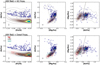 |
Fig. 1. Distribution of [N/Fe] vs. [Fe/H], [Al/Fe] vs. [Mg/Fe], and [Mg/Mn] vs. [Al/Fe] for the newly identified N-rich stars (navy) compared to GC stars (black dashed contours) from Mészáros et al. (2020), LMC (solid black contours), SMC (cyan dashed contours), and Sgr (solid red contours) stars from Helmi et al. (2018) with ASPCAP abundance information. The black dashed lines roughly define the criterion to “distinguish” in situ from accreted populations, similar to that as defined in Das et al. (2020) and Horta et al. (2021). Also included are kernel density estimation (KDE) models showing the density of objects belonging to the MW. The continuous black line in the first column represents the fourth order polynomial fit at the 4σ level selection criterion for N-rich stars as described in the text. Typical error bars are shown as black plus symbols in each panel. |
Description of the columns of the catalog containing the 149 newly identified N-rich stars.
Table 1 also lists five newly identified N-rich star candidates toward the SMC (three stars: 2M01055438−6833068, 2M01021954−7147493, and 2M00592789−6943291) and LMC (two stars: 2M05023164−7157181 and 2M05481230−7937052), which display similar physical properties to that seen in the stars of these systems. We do not provide orbital calculations for these stars because of the reasons provided in Sect. 6. These stars have been cataloged as Orbital_Sense == “Unknow/LMC-Candidate” and Orbital_Sense == “Unknow/SMC-Candidate”.
N-rich stars in Table 1 with Orbital_Sense == “prograde/HVNS-Candidate”, have been classified as hypervelocity N-rich star (HVNS) candidates. While N-rich stars in our sample with unreliable orbital solutions have been tagged as Orbital_Sense == “Unknow”, stars in different Galactic orbital configurations have been classified as Orbital_Sense == “P–R” to refer to the orbits changing their sense of motion from prograde to retrograde (P–R) during the integration time and vice versa, as Orbital_Sense == “Prograde” to highlight those stars in a prograde orbital configuration, and as Orbital_Sense == “Retrograde” to refer to those that lie in retrograde orbits. We characterize this newly identified N-rich population in Sect. 6.
It is also important to note that none of the 149 N-rich candidates without strong carbon enhancement have a particularly strong variability in their radial velocity over the period of the APOGEE-2 observations, thus limiting the possible orbital properties than can be detected in our data. Those sources with available multi-epoch observations exhibit a typical Vscatter < 0.9 km s−1, with the exception of three sources, which show a slightly high Vscatter between 1.64 and 2.6 km s−1. We also found no matches with the ASAS-SN Catalog of Variable Stars (Jayasinghe et al. 2021).
Although we have not found strong evidence for a binary companion or a pulsating variable star as of yet, we cannot rule out the possibility that some of these stars were members of a binary system in the past (see e.g., Fernández-Trincado et al. 2019c), or they could likely be part of the semi-regular (SR) variable populations (see e.g., Fernández-Trincado et al. 2020b). Therefore, long-term radial-velocity monitoring for all the identified N-rich stars is currently being carried out with the SDSS-V panoptic spectroscopic survey (Kollmeier et al. 2017) which, with a baseline that is better (≲6 months) than that of the APOGEE-2 DR 17 survey, would naturally be the best course to establish the number of such objects that formed through the binary channel or that currently belong to a kind of pulsating variable.
Table 2 summarizes the nearly complete census in APOGEE of N-rich field stars, for a grand total of ∼412 unique carbon-depleted N-rich candidates across the MW. It is expected that this number will increase further once the results from the new Milky Way Mapper (MWM) program of SDSS-V (Kollmeier et al. 2017) are published. Table 2 does not include the recent exploration by Phillips et al. (2022), which reports on the detection of two N-rich stars along the Palomar 5 Stream. These two stars were already identified previously by Martell et al. (2016) for 2M15204588+0055032, suggested as potential extra-tidal material of Palomar 5 in Fernández-Trincado et al. (2019b) for 2M15183589+0027100, and confirmed as members of the Palomar 5 Stream by the STREAMFINDER algorithm in Ibata et al. (2021). Table 3 lists the APOGEE ids and origin on the literature of the 412 compiled APOGEE N-rich stars.
Census updated of ∼412 unique field carbon-depleted N-rich ([C/Fe] < +0.15; [N/Fe] ≳ +0.5) stars in the APOGEE survey.
Compilation of the 412 N-rich stars identified thus far in the APOGEE survey.
Finally, we found that there are no known GCs within an angular separation of 1.5 × rtidal, GC arcmin out of the 149 newly reported N-rich stars in our sample, and there is not an association with the newly discovered stellar streams in the Gaia universe Ibata et al. (2021). However, some of them could be made up of dissipated GCs, which is investigated in detail by assessing other chemical species not accessible from the APOGEE-2 survey.
5. Elemental abundance analysis
In this section we analyze the chemical properties of the newly identified N-rich stars alongside the MW halo and disk, the LMC and SMC members, the Sagittarius spheroidal dwarf galaxy (Sgr), and GC members, in the chemical diagnostic plans of [N/Fe] versus [Fe/H], [Al/Fe] versus [Mg/Fe], and [Mg/Mn] versus [Al/Fe]. Our sample selection of LMC, SMC, and Sgr members was obtained by cross-matching the catalogs from Helmi’s web service2 (Gaia Collaboration 2018) against the APOGEE-2 DR 17 catalog (Abdurro’uf et al. 2022), and adopting the quality cuts described in Sect. 3. GC sources were adopted from Mészáros et al. (2020, 2021), but we adopted the APOGEE-2/ASPCAP DR 17 abundance determinations in order to avoid the systematic elemental abundances produced between BACCHUS (Masseron et al. 2016) and ASPCAP (García Pérez et al. 2016), as our sample relies on abundance ratios determined from the ASPCAP pipeline.
Figure 1 summarizes the elemental properties of the 149 newly identified N-rich red giant stars. The first column of the panels in this figure shows that the [N/Fe] abundance ratio of the N-rich stars is more compatible with the nitrogen-enriched GC population, rather than the LMC, SMC, and Sgr populations.
The second column of panels in Fig. 1 reveals that there appears to be at least two main groups in the [Mg/Fe] vs. [Al/Fe] plane, where [Al/Fe] is anticorrelated with [Mg/Fe], similar to what is seen in GC populations, primarily for [Al/Fe] ≳ 0, and where it also overlaps with the main bulk of ME stars. While the second group of N-rich stars with subsolar [Al/Fe] < 0 fall within the group dominated by the dwarf members plus GC populations with low-aluminum enrichment more likely the first-generation of GC stars as envisioned by Mészáros et al. (2020). The third column of panels in Fig. 1 shows [Mg/Mn] vs. [Al/Fe], as originally envisioned by Das et al. (2020). The newly identified N-rich populations expand the same locus of that chemical plane deemed to contain GC populations, even (in)outside the “accreted” population area defined by Das et al. (2020) which runs roughly above [Mg/Mn] > +0.25 and [Al/Fe] ≲ +0.2.
While Das et al. (2020) and Horta et al. (2021) suggest that the [Al/Fe]–[Mg/Mn] plane could be used to identify stellar populations that formed ex situ, some caution is recommended since metal-poor ([Fe/H] ≲ −0.7) nitrogen-enriched populations that likely formed ex situ share the same locus as the in situ MW population in this plane. In particular, for subsolar [Al/Fe], there is a mix of stellar populations belonging to GCs and dwarf populations.
6. Dynamical properties of selected N-rich stars
We examined the kinematic and dynamical properties of the newly identified N-rich stars by making use of the GravPot163 model (Fernández-Trincado 2017), and computing the ensemble of orbits integrated over a 3 Gyr time span. For the orbit calculations, we assumed a bar pattern speed of 41 ± 10 km s−1 kpc−1 (Sanders et al. 2019; Bovy et al. 2019). We note that our model has some limitations in the processes considered; for example, secular changes in the adopted MW potential as well as dynamical friction are not included.
The orbit calculations were performed by adopting a simple Monte Carlo approach that considers the errors of the observables. The resulting values and their errors were taken as the 16th, 50th, and 84th percentiles from the generated distributions. Heliocentric distances were estimated with the Bayesian StarHorse code (see e.g., Anders et al. 2019; Queiroz et al. 2018, 2020, 2021) as part of the APOGEE_STARHORSE Value Added Catalog4, proper motions are from Gaia EDR 3 (Gaia Collaboration 2021), and radial velocities are from the APOGEE-2 DR 17 database.
Figure 2 shows the resulting kinematic properties and orbital elements for 124 out of 149 stars in our sample which have a Gaia re-normalized unit weight error (RUWE) of less than 1.4 (indicating the high quality of their astrometric solutions), and uncertainties on the heliocentric distances of less than 20%. It is important to note that five potential N-rich SMC and LMC members were excluded from our dynamical analysis; as our MW model does not take the Magellanic Clouds’ contribution to the global gravitational potential into account, their orbital elements will be more uncertain.
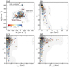 |
Fig. 2. Galactocentric radial (VR) and azimuthal (Vϕ) velocity, and orbital-element properties for the newly identified N-rich stars. The color-coding of the symbols in the panels is based on their [Fe/H], while the gray background shading represents the KDE model of the overlaid points, excluding the HVNS candidates (see text). The distribution of the velocity component VR vs. Vϕ is shown in panel a. The blue dashed line represents the approximate region for sources with the Gaia-Enceladus-Sausage-like kinematics in VR vs. Vϕ, based on Belokurov et al. (2018). The area occupied by disk-like stars is also highlighted with the empty black circle. The perigalactic (b), apogalactic distances (c), and the maximum vertical excursion (d) from the Galactic plane as a function of the orbital eccentricity are shown. Black up-tick symbols mark the stars with likely chaotic behavior, i.e., those with orbits that change their direction of motion from prograde to retrograde (and vice versa) with respect to the direction of Galactic rotation, while the small, empty black concentric symbols indicate the stars with retrograde orbits. Uncertainties are shown as gray plus symbols in each panel. The large star symbols mark the two HVNS candidates assuming the Bayesian StarHorse heliocentric distance estimations, while the large hexagonal markers refer to the same stars with Bailer-Jones heliocentric distance estimations. |
6.1. Kinematical properties
Figure 2 reveals that a significant fraction (65%; 80 stars) lie within the fraction dominated by Gaia-Enceladus-Sausage-like (GES-like; Belokurov et al. 2018; Helmi et al. 2018) stars and a halo-like population with Vϕ < 100 km s−1, which exhibit a typical azimuthal velocity uncertainty below 40 km s−1, with the exception of 2M16053258−4502140 exhibiting a relatively large azimuthal velocity uncertainty of Vϕ = −264 ± 163 km s−1, but it is clearly well separated kinematically from the GES-like component and disk populations (see Fig. 2). While 34% (42 stars) of the N-rich stars exhibit disk-like kinematics, with an azimuthal velocity of Vϕ > 100 km s−1 with typical uncertainties < 35 km s−1 – with the exception of 2M06243113+4213097 exhibiting a large uncertainty in Vϕ ∼ 237 ± 73 km s−1 – they are still related to the disk-like kinematic population. However, as is described below, the newly identified N-rich stars cover a wide range of dynamical characteristics with overlapping Galactocentric radial and azimuthal velocities.
6.2. Dynamical properties
A more elaborate inspection of their orbital elements reveal that there are at least four main groups of N-rich stars in our sample, whose kinematic distributions are shown in Fig. 3. The first group (Group #1) is dominated by a significant fraction (72 out of 124 stars) of N-rich stars which lie on pure prograde orbits with an azimuthal velocity of Vϕ ≳ −50 km s−1.
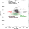 |
Fig. 3. Same as Fig. 2a, but here showing the KDE models of the newly identified N-rich stars confined to four main groups (see text). HVNS candidates (Group #4; 2 stars) are shown as empty black star symbols for the assumed Bayesian StarHorse distances and as empty black hexagonal symbols by adopting the Bailer-Jones distances, while N-rich stars in prograde (Group #1; 72 stars), retrograde (Group #2; 25 stars), and P–R (Group #3; 25 stars) orbital configurations are represented by the gray, green, and red contours, respectively. |
A second group (Group #2) is made up of 25 out of 124 N-rich stars which exhibit Vϕ < 100 km s−1. They also have a retrograde orbital configuration with respect to the rotation of the Galactic bar.
A third group (Group #3) composed of 25 out of 124 N-rich stars with Galactic azimuthal velocities ranging from −150 km s−1 ≲ Vϕ ≲ 150 km s−1 exhibit an unusual dynamical behavior, that is to say they are in the so-called P–R orbital configuration which changes their sense of motion from prograde to retrograde during the integration time and vice versa, which could also be related to chaotic behavior. Further, for these three groups, we find no strong correlation between their orbital elements and [Fe/H], which could be indicative of an early chaotic phase of the evolution of the MW, as well.
In addition, the N-rich stars occupying the GES-like component in Fig. 2 are dominated by a wide range of orbital configurations (including P–R, prograde and retrograde orbits), and they are almost completely confined to eccentricities larger than 0.65 peaking at ∼0.95, similar to that of the GES-like kinematic substructure identified by Naidu et al. (2020).
A fourth group (Group #4) is made up of two N-rich outliers in the Vϕ vs. VR plane at Vϕ > 600 km s−1. We refer to these stars as HVNS, and they likely form as part of the intriguing subgroup of the high-velocity stars (Hawkins et al. 2015, and references therein) readers are encouraged to refer to the discussion in Sect. 7.
Figure 2 also reveals that most of the metal-poor N-rich stars lie on high-eccentricity orbits with large vertical excursions above the Galactic plane, with some noticeable evidence of N-rich stars that likely formed in the outer halo, while the most metal-rich N-rich stars lie on prograde, low-eccentricity, inner halo- and disk-like orbital configurations. Interestingly, two (2M06243113+4213097 and 2M08534023−2554252) of the most metal-rich N-rich stars exhibit near circular orbital configurations in the outer disk of the MW, suggesting that they might have been formed in situ from material chemically self-enriched by a first generation of stars in the outer disk, or they could have formed from a GC disruption in the inner Galaxy and radially migrated to their current location and/or are trapped by disk ripples (Xu et al. 2015).
7. Hypervelocity N-rich star (HVNS) candidates
Strikingly, we also identified two N-rich stars with a high azimuthal velocity of Vϕ > 600 km s−1. Thus, these could be classified as atypical fast-moving N-rich stars likely escaping the MW potential, with the exception of the N-rich star 2M17025992−3537464 which exhibits a larger uncertainty in Vϕ ∼ 540 km s−1 overlapping with the kinematic of typical disk stars. We have classified these two stars as HVNS candidates.
Figure 4 reveals that the predicted orbital configurations of these HVNS candidates are racing through space at above the escape speed of the MW, having a perigalactic distance of rperi ∼ 11.7 ± 0.87 kpc (2M19175783−1343049) and rperi ∼ 17.09 ± 2.98 kpc (2M17025992−3537464), clearly indicating that they did not originate in the Galactic Center. However, their atypical chemistry suggests that these HVNS candidates likely have a GC formation site.
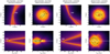 |
Fig. 4. Ensemble of ten thousand orbits for the two HVNS candidates 2M17025992−3537464 and 2M19175783−1343049, projected on the equatorial (top) and meridional (bottom) Galactic planes in the inertial reference frame with a bar pattern speed of 41 ± 10 km s−1 kpc−1, and time-integrated forward and backward over 1 Gyr. The yellow and orange colors correspond to more probable regions of the space, which are most frequently crossed by the simulated orbits. The black dashed and solid black lines show the 50th percentile for the forward and backward orbital path, respectively. The top panels show, for guidance, a MW bulge (solid white circle) and disk (white dashed circle) radius of ∼3.5 kpc (Barbuy et al. 2018) and ∼15 kpc, respectively. While the MW disk extension until ∼15 kpc is also denoted by a thick white line in the bottom panels. Columns (1) and (3) show the orbital configurations by assuming the Bayesian StarHorse distances, whilst Cols. (2) and (4) display the predicted orbits by adopting the Bailer-Jones geometric distances. |
These HVNS stars could have been produced via different physical processes, including the three-body encounters at the center of a GC; which through a process known as resonance scattering a binary star in the stellar cluster can capture a star in the cluster (thus forming a bound triple system), and after some time one of the stars (likely the HVNS) is ejected, or via flyby where a captured HVNS is ejected in the interaction (see e.g., Hut & Bahcall 1983; Pichardo et al. 2012; Fernández-Trincado et al. 2016b). This finding could aid in providing useful information about the environments from which the high-velocity halo stars are produced.
It is also important to note that Bailer-Jones et al. (2021) provide estimated heliocentric distances for these two stars which put them closer to the Sun (d⊙ < 6.5 kpc) than those estimated with the Bayesian StarHorse code (d⊙ > 19 kpc). Figures 2–4 reveal that adopting closer heliocentric distances for 2M19175783−1343049 and 2M17025992−3537464 puts these stars in an orbital configuration which inhabits the inner regions of the Galactic bulge in prograde and high eccentric (≳0.6) orbits, overlapping with the kinematic properties of the GES-like component (Vϕ < 100 km s−1).
However, the estimated distances from Bailer-Jones et al. (2021) for these two stars should be more uncertain as they should be dominated by a weak prior for a density distribution of the Galaxy, thus the priors would make us expect for these stars to be much closer than they truly are, producing unrealistic distances. Thus, it is likely that the distances from the Bailer-Jones catalog for 2M19175783−1343049 and 2M17025992−3537464 should just be following the priors. In addition, the Bayesian StarHorse code provides smaller uncertainties at larger ranges compared to the Bailer-Jones catalog. Therefore, we decided to use the Bayesian StarHorse distances derived by Queiroz et al. (2021) as the primary distance set for this work, also based on their better extinction treatment. However, with the upcoming Gaia DR3, we will be able to constrain the distances and proper motions better for these two HVNS candidates.
8. Conclusions
We report on the discovery of 149 newly identified carbon-depleted ([C/Fe] < +0.15) N-rich stars over a wide range of metallicities (−1.8 < [Fe/H] < −0.7) for a grand total of ∼412 N-rich stars across the MW. Similar to the previously identified nitrogen-enhanced population, the new one exhibits elemental abundances comparable to those exclusively seen in GC environments.
We also examined the position of the newly identified N-rich stars in the [Al/Fe] versus [Mg/Mn] plane as envisioned by Das et al. (2020), finding that N-rich stars occupy a wide range at and beyond the locus deemed to contain an “accreted” population ([Al/Fe] ≲ 0 and [Mg/Mn] ≳ +0.25) and to that dominated by an in situ population of the MW. This suggests that the region occupied by the in situ population of the MW has a non-negligible presence of stars with unusual elemental abundances, likely associated to tidal stripping and/or the disruption of GCs over different epochs of evolution of the MW. The diverse dynamical and kinematical characteristics of the newly identified N-rich stars reveal that they do not share the same birthplaces in the MW, and that some of them could be the debris of GCs that were fully or partially destroyed during previous major merger accretion events such as the GES.
Acknowledgments
The author is grateful for the enlightening feedback from the anonymous referee. J.G.F.-T. gratefully acknowledges the grant support provided by Proyecto Fondecyt Iniciación No. 11220340, and also from ANID Concurso de Fomento a la Vinculación Internacional para Instituciones de Investigación Regionales (Modalidad corta duración) Proyecto No. FOVI210020. J.G.F.-T. and D.G.D. gratefully acknowledge the grant support from the Joint Committee ESO-Government of Chile 2021 (ORP 023/2021). T.C.B. acknowledges partial support for this work from grant PHY 14-30152: Physics Frontier Center / JINA Center for the Evolution of the Elements (JINA-CEE), awarded by the US National Science Foundation. B.B. acknowledges grants from FAPESP, CNPq and CAPES – Financial code 001. D.M. gratefully acknowledges support by the ANID BASAL projects ACE210002 and FB210003, and Fondecyt Project No. 1220724. E.R.G. acknowledges support from ANID PhD scholarship No. 21210330. S.V. gratefully acknowledges the support provided by Fondecyt regular n. 1220264. D.G. gratefully acknowledges support from the ANID BASAL project ACE210002. D.G. also acknowledges financial support from the Dirección de Investigación y Desarrollo de la Universidad de La Serena through the Programa de Incentivo a la Investigación de Académicos (PIA-DIDULS). This work has made use of data from the European Space Agency (ESA) mission Gaia (http://www.cosmos.esa.int/gaia), processed by the Gaia Data Processing and Analysis Consortium (DPAC, http://www.cosmos.esa.int/web/gaia/dpac/consortium). Funding for the DPAC has been provided by national institutions, in particular the institutions participating in the Gaia Multilateral Agreement. Funding for the Sloan Digital Sky Survey IV has been provided by the Alfred P. Sloan Foundation, the U.S. Department of Energy Office of Science, and the Participating Institutions. SDSS-IV acknowledges support and resources from the Center for High-Performance Computing at the University of Utah. The SDSS web site is www.sdss.org. SDSS-IV is managed by the Astrophysical Research Consortium for the Participating Institutions of the SDSS Collaboration including the Brazilian Participation Group, the Carnegie Institution for Science, Carnegie Mellon University, the Chilean Participation Group, the French Participation Group, Harvard-Smithsonian Center for Astrophysics, Instituto de Astrofìsica de Canarias, The Johns Hopkins University, Kavli Institute for the Physics and Mathematics of the Universe (IPMU)/University of Tokyo, Lawrence Berkeley National Laboratory, Leibniz Institut für Astrophysik Potsdam (AIP), Max-Planck-Institut für Astronomie (MPIA Heidelberg), Max-Planck-Institut für Astrophysik (MPA Garching), Max-Planck-Institut für Extraterrestrische Physik (MPE), National Astronomical Observatory of China, New Mexico State University, New York University, University of Notre Dame, Observatório Nacional/MCTI, The Ohio State University, Pennsylvania State University, Shanghai Astronomical Observatory, United Kingdom Participation Group, Universidad Nacional Autónoma de México, University of Arizona, University of Colorado Boulder, University of Oxford, University of Portsmouth, University of Utah, University of Virginia, University of Washington, University of Wisconsin, Vanderbilt University, and Yale University. This work has made use of data from the European Space Agency (ESA) mission Gaia (http://www.cosmos.esa.int/gaia), processed by the Gaia Data Processing and Analysis Consortium (DPAC, http://www.cosmos.esa.int/web/gaia/dpac/consortium). Funding for the DPAC has been provided by national institutions, in particular the institutions participating in the Gaia Multilateral Agreement.
References
- Abdurro’uf, Accetta, K., Aerts, C., et al. 2022, ApJS, 259, 35 [NASA ADS] [CrossRef] [Google Scholar]
- Alvarez, R., & Plez, B. 1998, A&A, 330, 1109 [NASA ADS] [Google Scholar]
- Anders, F., Chiappini, C., Santiago, B. X., et al. 2018, A&A, 619, A125 [NASA ADS] [CrossRef] [EDP Sciences] [Google Scholar]
- Anders, F., Khalatyan, A., Chiappini, C., et al. 2019, A&A, 628, A94 [NASA ADS] [CrossRef] [EDP Sciences] [Google Scholar]
- Anguiano, B., Zucker, D. B., Scholz, R. D., et al. 2015, MNRAS, 451, 1229 [NASA ADS] [CrossRef] [Google Scholar]
- Bailer-Jones, C. A. L., Rybizki, J., Fouesneau, M., Demleitner, M., & Andrae, R. 2021, AJ, 161, 147 [Google Scholar]
- Barbá, R. H., Minniti, D., Geisler, D., et al. 2019, ApJ, 870, L24 [CrossRef] [Google Scholar]
- Barbuy, B., Chiappini, C., & Gerhard, O. 2018, ARA&A, 56, 223 [Google Scholar]
- Baumgardt, H., & Vasiliev, E. 2021, MNRAS, 505, 5957 [NASA ADS] [CrossRef] [Google Scholar]
- Beaton, R. L., Oelkers, R. J., Hayes, C. R., et al. 2021, AJ, 162, 302 [NASA ADS] [CrossRef] [Google Scholar]
- Bekki, K. 2019, MNRAS, 490, 4007 [Google Scholar]
- Belokurov, V., Erkal, D., Evans, N. W., Koposov, S. E., & Deason, A. J. 2018, MNRAS, 478, 611 [Google Scholar]
- Blanco-Cuaresma, S., Soubiran, C., Heiter, U., & Jofré, P. 2014, A&A, 569, A111 [CrossRef] [EDP Sciences] [Google Scholar]
- Blanton, M. R., Bershady, M. A., Abolfathi, B., et al. 2017, AJ, 154, 28 [Google Scholar]
- Bovy, J., Leung, H. W., Hunt, J. A. S., et al. 2019, MNRAS, 490, 4740 [Google Scholar]
- Bowen, I. S.,& Vaughan, A. H. J. 1973, Appl. Opt., 12, 1430 [NASA ADS] [CrossRef] [Google Scholar]
- Carollo, D., Martell, S. L., Beers, T. C., & Freeman, K. C. 2013, ApJ, 769, 87 [NASA ADS] [CrossRef] [Google Scholar]
- Chiba, M., & Beers, T. C. 2000, AJ, 119, 2843 [NASA ADS] [CrossRef] [Google Scholar]
- Cunha, K., Smith, V. V., Hasselquist, S., et al. 2017, ApJ, 844, 145 [Google Scholar]
- Da Costa, G. S., & Coleman, M. G. 2008, AJ, 136, 506 [CrossRef] [Google Scholar]
- Das, P., Hawkins, K., & Jofré, P. 2020, MNRAS, 493, 5195 [NASA ADS] [CrossRef] [Google Scholar]
- Fernández-Trincado, J. G. 2017, PhD Thesis, University of Franche-Comté, France [Google Scholar]
- Fernández-Trincado, J. G., Robin, A. C., Vieira, K., et al. 2015a, A&A, 583, A76 [NASA ADS] [CrossRef] [EDP Sciences] [Google Scholar]
- Fernández-Trincado, J. G., Vivas, A. K., Mateu, C. E., et al. 2015b, A&A, 574, A15 [NASA ADS] [CrossRef] [EDP Sciences] [Google Scholar]
- Fernández-Trincado, J. G., Robin, A. C., Moreno, E., et al. 2016a, ApJ, 833, 132 [Google Scholar]
- Fernández-Trincado, J. G., Robin, A. C., Reylé, C., et al. 2016b, MNRAS, 461, 1404 [Google Scholar]
- Fernández-Trincado, J. G., Zamora, O., García-Hernández, D. A., et al. 2017, ApJ, 846, L2 [Google Scholar]
- Fernández-Trincado, J. G., Beers, T. C., Placco, V. M., et al. 2019a, ApJ, 886, L8 [Google Scholar]
- Fernández-Trincado, J. G., Beers, T. C., Tang, B., et al. 2019b, MNRAS, 488, 2864 [NASA ADS] [Google Scholar]
- Fernández-Trincado, J. G., Mennickent, R., Cabezas, M., et al. 2019c, A&A, 631, A97 [NASA ADS] [CrossRef] [EDP Sciences] [Google Scholar]
- Fernández-Trincado, J. G., Zamora, O., Souto, D., et al. 2019d, A&A, 627, A178 [Google Scholar]
- Fernández-Trincado, J. G., Beers, T. C., & Minniti, D. 2020a, A&A, 644, A83 [Google Scholar]
- Fernández-Trincado, J. G., Beers, T. C., Minniti, D., et al. 2020b, ApJ, 903, L17 [Google Scholar]
- Fernández-Trincado, J. G., Beers, T. C., Minniti, D., et al. 2020c, A&A, 643, L4 [Google Scholar]
- Fernández-Trincado, J. G., Chaves-Velasquez, L., Pérez-Villegas, A., et al. 2020d, MNRAS, 495, 4113 [Google Scholar]
- Fernández-Trincado, J. G., Minniti, D., Beers, T. C., et al. 2020e, A&A, 643, A145 [Google Scholar]
- Fernández-Trincado, J. G., Beers, T. C., Barbuy, B., et al. 2021a, ApJ, 918, L9 [CrossRef] [Google Scholar]
- Fernández-Trincado, J. G., Beers, T. C., Minniti, D., et al. 2021b, A&A, 647, A64 [EDP Sciences] [Google Scholar]
- Fernández-Trincado, J. G., Beers, T. C., Minniti, D., et al. 2021c, A&A, 648, A70 [Google Scholar]
- Fernández-Trincado, J. G., Beers, T. C., Queiroz, A. B. A., et al. 2021d, ApJ, 918, L37 [CrossRef] [Google Scholar]
- Fernández-Trincado, J. G., Minniti, D., Souza, S. O., et al. 2021e, ApJ, 908, L42 [Google Scholar]
- Fernández-Trincado, J. G., Minniti, D., Garro, E. R., & Villanova, S. 2022a, A&A, 657, A84 [NASA ADS] [CrossRef] [EDP Sciences] [Google Scholar]
- Fernández-Trincado, J. G., Villanova, S., Geisler, D., et al. 2022b, A&A, 658, A116 [NASA ADS] [CrossRef] [EDP Sciences] [Google Scholar]
- Forbes, D. A. 2020, MNRAS, 493, 847 [Google Scholar]
- Gaia Collaboration (Helmi, A., et al.) 2018, A&A, 616, A12 [NASA ADS] [CrossRef] [EDP Sciences] [Google Scholar]
- Gaia Collaboration (Brown, A. G. A., et al.) 2021, A&A, 650, C3 [EDP Sciences] [Google Scholar]
- García Pérez, A. E., Allende Prieto, C., Holtzman, J. A., et al. 2016, AJ, 151, 144 [Google Scholar]
- Geisler, D., Villanova, S., O’Connell, J. E., et al. 2021, A&A, 652, A157 [NASA ADS] [CrossRef] [EDP Sciences] [Google Scholar]
- Gudin, D., Shank, D., Beers, T. C., et al. 2021, ApJ, 908, 79 [NASA ADS] [CrossRef] [Google Scholar]
- Gunn, J. E., Siegmund, W. A., Mannery, E. J., et al. 2006, AJ, 131, 2332 [NASA ADS] [CrossRef] [Google Scholar]
- Hanke, M., Koch, A., Prudil, Z., Grebel, E. K., & Bastian, U. 2020, A&A, 637, A98 [EDP Sciences] [Google Scholar]
- Hasselquist, S., Shetrone, M., Cunha, K., et al. 2016, ApJ, 833, 81 [Google Scholar]
- Hasselquist, S., Shetrone, M., Smith, V., et al. 2017, ApJ, 845, 162 [Google Scholar]
- Hasselquist, S., Carlin, J. L., Holtzman, J. A., et al. 2019, ApJ, 872, 58 [Google Scholar]
- Hawkins, K., Kordopatis, G., Gilmore, G., et al. 2015, MNRAS, 447, 2046 [CrossRef] [Google Scholar]
- Helmi, A. 2020, ARA&A, 58, 205 [Google Scholar]
- Helmi, A., White, S. D. M., de Zeeuw, P. T., & Zhao, H. 1999, Nature, 402, 53 [Google Scholar]
- Helmi, A., Babusiaux, C., Koppelman, H. H., et al. 2018, Nature, 563, 85 [Google Scholar]
- Holmbeck, E. M., Hansen, T. T., Beers, T. C., et al. 2020, ApJs, 249, 30 [NASA ADS] [CrossRef] [Google Scholar]
- Holtzman, J. A., Shetrone, M., Johnson, J. A., et al. 2015, AJ, 150, 148 [Google Scholar]
- Holtzman, J. A., Hasselquist, S., Shetrone, M., et al. 2018, AJ, 156, 125 [Google Scholar]
- Horta, D., Schiavon, R. P., Mackereth, J. T., et al. 2021, MNRAS, 500, 1385 [Google Scholar]
- Hut, P., & Bahcall, J. N. 1983, ApJ, 268, 319 [NASA ADS] [CrossRef] [Google Scholar]
- Ibata, R. A., Gilmore, G., & Irwin, M. J. 1994, Nature, 370, 194 [Google Scholar]
- Ibata, R. A., Bellazzini, M., Malhan, K., Martin, N., & Bianchini, P. 2019, Nat. Astron., 3, 667 [Google Scholar]
- Ibata, R., Malhan, K., Martin, N., et al. 2021, ApJ, 914, 123 [NASA ADS] [CrossRef] [Google Scholar]
- Jayasinghe, T., Kochanek, C. S., Stanek, K. Z., et al. 2021, MNRAS, 503, 200 [NASA ADS] [CrossRef] [Google Scholar]
- Johnson, J. A., Herwig, F., Beers, T. C., & Christlieb, N. 2007, ApJ, 658, 1203 [Google Scholar]
- Jönsson, H., Allende Prieto, C., Holtzman, J. A., et al. 2018, AJ, 156, 126 [Google Scholar]
- Karinkuzhi, D., & Goswami, A. 2015, MNRAS, 446, 2348 [NASA ADS] [CrossRef] [Google Scholar]
- Kemp, A. J., Casey, A. R., Miles, M. T., et al. 2018, MNRAS, 480, 1384 [NASA ADS] [CrossRef] [Google Scholar]
- Kisku, S., Schiavon, R. P., Horta, D., et al. 2021, MNRAS, 504, 1657 [NASA ADS] [CrossRef] [Google Scholar]
- Kollmeier, J. A., Zasowski, G., Rix, H. W., et al. 2017, ArXiv e-prints [arXiv:1711.03234] [Google Scholar]
- Koo, J.-R., Lee, Y. S., Park, H.-J., Kim, Y. K., & Beers, T. C. 2022, ApJ, 925, 35 [NASA ADS] [CrossRef] [Google Scholar]
- Koppelman, H. H., Helmi, A., Massari, D., Price-Whelan, A. M., & Starkenburg, T. K. 2019, A&A, 631, L9 [NASA ADS] [CrossRef] [EDP Sciences] [Google Scholar]
- Kruijssen, J. M. D., Pfeffer, J. L., Chevance, M., et al. 2020, MNRAS, 498, 2472 [NASA ADS] [CrossRef] [Google Scholar]
- Kunder, A., Bono, G., Piffl, T., et al. 2014, A&A, 572, A30 [NASA ADS] [CrossRef] [EDP Sciences] [Google Scholar]
- Kundu, R., Fernández-Trincado, J. G., Minniti, D., et al. 2019a, MNRAS, 489, 4565 [Google Scholar]
- Kundu, R., Minniti, D., & Singh, H. P. 2019b, MNRAS, 483, 1737 [Google Scholar]
- Kundu, R., Navarrete, C., Fernández-Trincado, J. G., et al. 2021, A&A, 645, A116 [EDP Sciences] [Google Scholar]
- Leon, S., Meylan, G., & Combes, F. 2000, A&A, 359, 907 [NASA ADS] [Google Scholar]
- Lind, K., Koposov, S. E., Battistini, C., et al. 2015, A&A, 575, L12 [NASA ADS] [CrossRef] [EDP Sciences] [Google Scholar]
- Lucey, M., Hawkins, K., Ness, M., et al. 2022, MNRAS, 509, 122 [Google Scholar]
- Majewski, S. R., Nidever, D. L., Smith, V. V., et al. 2012, ApJ, 747, L37 [NASA ADS] [CrossRef] [Google Scholar]
- Majewski, S. R., Schiavon, R. P., Frinchaboy, P. M., et al. 2017, AJ, 154, 94 [NASA ADS] [CrossRef] [Google Scholar]
- Malhan, K., Ibata, R. A., Sharma, S., et al. 2022, ApJ, 926, 107 [NASA ADS] [CrossRef] [Google Scholar]
- Marconi, M., Musella, I., Di Criscienzo, M., et al. 2014, MNRAS, 444, 3809 [NASA ADS] [CrossRef] [Google Scholar]
- Martell, S. L., Shetrone, M. D., Lucatello, S., et al. 2016, ApJ, 825, 146 [Google Scholar]
- Martin, N. F., Venn, K. A., Aguado, D. S., et al. 2022, Nature, 601, 45 [NASA ADS] [CrossRef] [Google Scholar]
- Masseron, T., García-Hernández, D. A., Mészáros, S., et al. 2019, A&A, 622, A191 [NASA ADS] [CrossRef] [EDP Sciences] [Google Scholar]
- Masseron, T., García-Hernández, D. A., Santoveña, R., et al. 2020a, Nat. Commun., 11, 3759 [NASA ADS] [CrossRef] [Google Scholar]
- Masseron, T., García-Hernández, D. A., Zamora, O., & Manchado, A. 2020b, ApJ, 904, L1 [NASA ADS] [CrossRef] [Google Scholar]
- Masseron, T., Merle, T., & Hawkins, K. 2016, Astrophysics Source Code Library [record ascl:1605.004] [Google Scholar]
- Mészáros, S., Masseron, T., García-Hernández, D. A., et al. 2020, MNRAS, 492, 1641 [Google Scholar]
- Mészáros, S., Masseron, T., Fernández-Trincado, J. G., et al. 2021, MNRAS, 505, 1645 [Google Scholar]
- Minniti, D., Fernández-Trincado, J. G., Ripepi, V., et al. 2018, ApJ, 869, L10 [Google Scholar]
- Myeong, G. C., Vasiliev, E., Iorio, G., Evans, N. W., & Belokurov, V. 2019, MNRAS, 488, 1235 [Google Scholar]
- Naidu, R. P., Tacchella, S., Mason, C. A., et al. 2020, ApJ, 892, 109 [NASA ADS] [CrossRef] [Google Scholar]
- Nidever, D. L., Holtzman, J. A., Allende Prieto, C., et al. 2015, AJ, 150, 173 [NASA ADS] [CrossRef] [Google Scholar]
- Pereira, C. B., Smith, V. V., Drake, N. A., et al. 2017, MNRAS, 469, 774 [NASA ADS] [CrossRef] [Google Scholar]
- Pereira, C. B., Drake, N. A., & Roig, F. 2019a, MNRAS, 488, 482 [NASA ADS] [CrossRef] [Google Scholar]
- Pereira, C. B., Holanda, N., Drake, N. A., & Roig, F. 2019b, AJ, 157, 70 [NASA ADS] [CrossRef] [Google Scholar]
- Phillips, S. G., Schiavon, R. P., Mackereth, J. T., et al. 2022, MNRAS, 510, 3727 [NASA ADS] [CrossRef] [Google Scholar]
- Pichardo, B., Moreno, E., Allen, C., et al. 2012, AJ, 143, 73 [NASA ADS] [CrossRef] [Google Scholar]
- Queiroz, A. B. A., Anders, F., Santiago, B. X., et al. 2018, MNRAS, 476, 2556 [Google Scholar]
- Queiroz, A. B. A., Anders, F., Chiappini, C., et al. 2020, A&A, 638, A76 [NASA ADS] [CrossRef] [EDP Sciences] [Google Scholar]
- Queiroz, A. B. A., Chiappini, C., Perez-Villegas, A., et al. 2021, A&A, 656, A156 [NASA ADS] [CrossRef] [EDP Sciences] [Google Scholar]
- Recio-Blanco, A., Rojas-Arriagada, A., de Laverny, P., et al. 2017, A&A, 602, L14 [NASA ADS] [CrossRef] [EDP Sciences] [Google Scholar]
- Romero-Colmenares, M., Fernández-Trincado, J. G., Geisler, D., et al. 2021, A&A, 652, A158 [NASA ADS] [CrossRef] [EDP Sciences] [Google Scholar]
- Sanders, J. L., Smith, L., & Evans, N. W. 2019, MNRAS, 488, 4552 [NASA ADS] [CrossRef] [Google Scholar]
- Santana, F. A., Beaton, R. L., Covey, K. R., et al. 2021, AJ, 162, 303 [NASA ADS] [CrossRef] [Google Scholar]
- Schiavon, R. P., Zamora, O., Carrera, R., et al. 2017, MNRAS, 465, 501 [Google Scholar]
- Shank, D., Beers, T. C., Placco, V. M., et al. 2022, ApJ, 926, 26 [NASA ADS] [CrossRef] [Google Scholar]
- Shetrone, M., Bizyaev, D., Lawler, J. E., et al. 2015, ApJs, 221, 24 [NASA ADS] [CrossRef] [Google Scholar]
- Simpson, J. D., & Martell, S. L. 2019, MNRAS, 490, 741 [NASA ADS] [CrossRef] [Google Scholar]
- Smith, V. V., Bizyaev, D., Cunha, K., et al. 2021, AJ, 161, 254 [NASA ADS] [CrossRef] [Google Scholar]
- Sneden, C. A. 1973, PhD Thesis, University of Texas [Google Scholar]
- Sollima, A. 2020, MNRAS, 495, 2222 [Google Scholar]
- Tang, B., Liu, C., Fernández-Trincado, J. G., et al. 2019, ApJ, 871, 58 [Google Scholar]
- Tang, B., Fernández-Trincado, J. G., Liu, C., et al. 2020, ApJ, 891, 28 [NASA ADS] [CrossRef] [Google Scholar]
- Vasiliev, E., & Baumgardt, H. 2021, MNRAS, 505, 5978 [NASA ADS] [CrossRef] [Google Scholar]
- Villanova, S., Geisler, D., Gratton, R. G., & Cassisi, S. 2014, ApJ, 791, 107 [Google Scholar]
- Wan, Z., Lewis, G. F., Li, T. S., et al. 2020, Nature, 583, 768 [Google Scholar]
- Wilson, J. C., Hearty, F. R., Skrutskie, M. F., et al. 2019, PASP, 131 [Google Scholar]
- Xu, Y., Newberg, H. J., Carlin, J. L., et al. 2015, ApJ, 801, 105 [Google Scholar]
- Yu, J., Tang, B., Fernández-Trincado, J. G., et al. 2021, ApJ, 913, 23 [NASA ADS] [CrossRef] [Google Scholar]
- Zamora, O., García-Hernández, D. A., Allende Prieto, C., et al. 2015, AJ, 149, 181 [CrossRef] [Google Scholar]
- Zasowski, G., Johnson, J. A., Frinchaboy, P. M., et al. 2013, AJ, 146, 81 [NASA ADS] [CrossRef] [Google Scholar]
- Zasowski, G., Cohen, R. E., Chojnowski, S. D., et al. 2017, AJ, 154, 198 [Google Scholar]
All Tables
Description of the columns of the catalog containing the 149 newly identified N-rich stars.
Census updated of ∼412 unique field carbon-depleted N-rich ([C/Fe] < +0.15; [N/Fe] ≳ +0.5) stars in the APOGEE survey.
All Figures
|
Fig. 1. Distribution of [N/Fe] vs. [Fe/H], [Al/Fe] vs. [Mg/Fe], and [Mg/Mn] vs. [Al/Fe] for the newly identified N-rich stars (navy) compared to GC stars (black dashed contours) from Mészáros et al. (2020), LMC (solid black contours), SMC (cyan dashed contours), and Sgr (solid red contours) stars from Helmi et al. (2018) with ASPCAP abundance information. The black dashed lines roughly define the criterion to “distinguish” in situ from accreted populations, similar to that as defined in Das et al. (2020) and Horta et al. (2021). Also included are kernel density estimation (KDE) models showing the density of objects belonging to the MW. The continuous black line in the first column represents the fourth order polynomial fit at the 4σ level selection criterion for N-rich stars as described in the text. Typical error bars are shown as black plus symbols in each panel. |
| In the text | |
|
Fig. 2. Galactocentric radial (VR) and azimuthal (Vϕ) velocity, and orbital-element properties for the newly identified N-rich stars. The color-coding of the symbols in the panels is based on their [Fe/H], while the gray background shading represents the KDE model of the overlaid points, excluding the HVNS candidates (see text). The distribution of the velocity component VR vs. Vϕ is shown in panel a. The blue dashed line represents the approximate region for sources with the Gaia-Enceladus-Sausage-like kinematics in VR vs. Vϕ, based on Belokurov et al. (2018). The area occupied by disk-like stars is also highlighted with the empty black circle. The perigalactic (b), apogalactic distances (c), and the maximum vertical excursion (d) from the Galactic plane as a function of the orbital eccentricity are shown. Black up-tick symbols mark the stars with likely chaotic behavior, i.e., those with orbits that change their direction of motion from prograde to retrograde (and vice versa) with respect to the direction of Galactic rotation, while the small, empty black concentric symbols indicate the stars with retrograde orbits. Uncertainties are shown as gray plus symbols in each panel. The large star symbols mark the two HVNS candidates assuming the Bayesian StarHorse heliocentric distance estimations, while the large hexagonal markers refer to the same stars with Bailer-Jones heliocentric distance estimations. |
| In the text | |
|
Fig. 3. Same as Fig. 2a, but here showing the KDE models of the newly identified N-rich stars confined to four main groups (see text). HVNS candidates (Group #4; 2 stars) are shown as empty black star symbols for the assumed Bayesian StarHorse distances and as empty black hexagonal symbols by adopting the Bailer-Jones distances, while N-rich stars in prograde (Group #1; 72 stars), retrograde (Group #2; 25 stars), and P–R (Group #3; 25 stars) orbital configurations are represented by the gray, green, and red contours, respectively. |
| In the text | |
|
Fig. 4. Ensemble of ten thousand orbits for the two HVNS candidates 2M17025992−3537464 and 2M19175783−1343049, projected on the equatorial (top) and meridional (bottom) Galactic planes in the inertial reference frame with a bar pattern speed of 41 ± 10 km s−1 kpc−1, and time-integrated forward and backward over 1 Gyr. The yellow and orange colors correspond to more probable regions of the space, which are most frequently crossed by the simulated orbits. The black dashed and solid black lines show the 50th percentile for the forward and backward orbital path, respectively. The top panels show, for guidance, a MW bulge (solid white circle) and disk (white dashed circle) radius of ∼3.5 kpc (Barbuy et al. 2018) and ∼15 kpc, respectively. While the MW disk extension until ∼15 kpc is also denoted by a thick white line in the bottom panels. Columns (1) and (3) show the orbital configurations by assuming the Bayesian StarHorse distances, whilst Cols. (2) and (4) display the predicted orbits by adopting the Bailer-Jones geometric distances. |
| In the text | |
Current usage metrics show cumulative count of Article Views (full-text article views including HTML views, PDF and ePub downloads, according to the available data) and Abstracts Views on Vision4Press platform.
Data correspond to usage on the plateform after 2015. The current usage metrics is available 48-96 hours after online publication and is updated daily on week days.
Initial download of the metrics may take a while.