| Issue |
A&A
Volume 665, September 2022
|
|
|---|---|---|
| Article Number | A53 | |
| Number of page(s) | 20 | |
| Section | Stellar structure and evolution | |
| DOI | https://doi.org/10.1051/0004-6361/202142670 | |
| Published online | 08 September 2022 | |
The eccentric millisecond pulsar, PSR J0955−6150
I. Pulse profile analysis, mass measurements, and constraints on binary evolution
1
SKA Observatory, Jodrell Bank, Lower Withington, Macclesfield SK11 9FT, UK
e-mail: This email address is being protected from spambots. You need JavaScript enabled to view it.
2
South African Radio Astronomy Observatory, 2 Fir Street, Black River Park, Observatory 7925, South Africa
3
Department of Physics and Astronomy, University of the Western Cape, Bellville, Cape Town 7535, South Africa
4
Max-Planck-Institut für Radioastronomie, Auf dem Hügel 69, 53121 Bonn, Germany
e-mail: This email address is being protected from spambots. You need JavaScript enabled to view it.
5
Department of Materials and Production, Aalborg University, Skjernvej 4A, 9220 Aalborg Øst, Denmark
6
Centre for Astrophysics and Supercomputing, Swinburne University of Technology, PO Box 218, Hawthorn, VIC 3122, Australia
7
ARC Centre of Excellence for Gravitational Wave Discovery (OzGrav), Hawthorn, Australia
8
INAF – Osservatorio Astronomico di Cagliari, Via della Scienza 5, 09047 Selargius, Italy
9
Department of Astrophysics, University of Oxford, Denys Wilkinson building, Keble Road, Oxford OX1 3RH, UK
10
Department of Physics and Electronics, Rhodes University, PO Box 94, Grahamstown 6140, South Africa
11
CSIRO, Space and Astronomy, PO Box 76, Epping, NSW 1710, Australia
12
Jodrell Bank Centre for Astrophysics, Department of Physics and Astronomy, University of Manchester, Manchester M13 9PL, UK
13
Dept. of Physics and Astronomy, University of British Columbia, 6224 Agricultural Road, Vancouver, BC V6T 1Z1, Canada
14
Institute for Radio Astronomy & Space Research, Auckland University of Technology, Private Bag 92006, Auckland 1142, New Zealand
Received:
15
November
2021
Accepted:
28
February
2022
Abstract
Context. PSR J0955−6150 is a member of an enigmatic class of eccentric millisecond pulsar (MSP) and helium white dwarf (He WD) systems (eMSPs), whose binary evolution is poorly understood and believed to be strikingly different to that of traditional MSP+He WD systems in circular orbits.
Aims. Measuring the masses of the stars in this system is important for testing the different hypotheses for the formation of eMSPs.
Methods. We carried out timing observations of this pulsar with the Parkes radio telescope using the 20 cm multibeam and ultra-wide bandwidth low-frequency (UWL) receivers, and the L-band receiver of the MeerKAT radio telescope. The pulse profiles were flux and polarisation calibrated, and a rotating-vector model (RVM) was fitted to the position angle of the linear polarisation of the combined MeerKAT data. Pulse times of arrival (ToAs) were obtained from these using standard pulsar analysis techniques and analysed using the TEMPO2 timing software.
Results. Our observations reveal a strong frequency evolution of this MSP’s intensity, with a flux density spectral index (α) of −3.13(2). The improved sensitivity of MeerKAT resulted in a greater than tenfold improvement in the timing precision obtained compared to our older Parkes observations. This, combined with the eight-year timing baseline, has allowed precise measurements of a very small proper motion and three orbital post-Keplerian parameters, namely the rate of advance of periastron, ω̇ = 0.00152(1) deg yr−1, and the orthometric Shapiro delay parameters, h3 = 0.89(7) μs and ς = 0.88(2). Assuming general relativity, we obtain Mp = 1.71(2) M⊙ for the mass of the pulsar and Mc = 0.254(2) M⊙ for the mass of the companion; the orbital inclination is 83.2(4) degrees. Crucially, assuming that the position angle of the linear polarisation follows the RVM, we find that the spin axis has a misalignment relative to the orbital angular momentum of > 4.8deg at 99% confidence level.
Conclusions. While the value of Mp falls well within the wide range observed in eMSPs, Mc is significantly smaller than expected from several formation hypotheses proposed, which are therefore unlikely to be correct and can be ruled out; Mc is also significantly different from the expected value for an ideal low mass X-ray binary evolution scenario. If the misalignment between the spin axis of the pulsar and the orbital angular momentum is to be believed, it suggests that the unknown process that created the orbital eccentricity of the binary was also capable of changing its orbital orientation, an important evidence for understanding the origin of eMSPs.
Key words: stars: neutron / binaries: general / pulsars: individual: PSR J0955–6150
© ESO 2022
1. Introduction
Radio pulsars are unique objects in astronomy: they are neutron stars (NSs) that emit a regular train of radio pulses whose times of arrival (TOAs) at the telescope can be measured with great precision (Lorimer & Kramer 2012). This allows the determination of extremely precise spin periods (sometimes better than a few femtoseconds), the rate of variation in this spin period, and astrometric parameters such as positions and proper motions that are precise to microarcseconds, similar to the precision obtained from very large baseline interferometry (VLBI). In the case of pulsars in binary systems, pulsar timing allows exquisitely precise measurements of their orbital motion, which can be used for precise measurements of the components of the binary (Özel & Freire 2016) and tests of gravity theories (Wex et al. 2014; Kramer et al. 2021a).
The MeerKAT 64-dish array (Jonas 2009) now provides excellent sensitivity (and thus timing precision) for Southern radio pulsars. Precision pulsar timing is carried out under the MeerTime large science project (LSP; Bailes et al. 2020); the first results are extremely promising and show a performance that is significantly better than expected. Within the MeerTime LSP, there is a programme targeting relativistic binary pulsars called RelBin. The objective of this programme is to use the excellent timing precision provided by the MeerKAT to improve the measurement or detection of new relativistic effects in the orbital motion of known binary pulsars, with the aim of increasing the number of NSs with precise mass measurements and increasing the number, nature, and precision of pulsar tests of gravity theories (for details, see Kramer et al. 2021b).
One of the early additions to the RelBin programme was PSR J0955−6150, a binary millisecond pulsar (MSP) with a low-mass companion and a 24.6 d orbit with an unusual eccentricity (e = 0.11) that was discovered with the CSIRO Parkes 64 m radio telescope (recently given the indigenous Wiradjuri name Murriyang) in a survey of unassociated Fermi sources (Camilo et al. 2015). In that paper, no phase-coherent timing solution was presented for this pulsar, owing to its extreme faintness, only an orbital solution derived from the observed variation in the spin period (the Doppler method). We were able to derive a phase-connected timing solution for this pulsar based on its Parkes long-term timing data. Even at that stage, with orbital parameters thousands of times more precise than those derived from the Doppler method, we could still only detect one relativistic effect in the orbit (the advance of periastron, which proceeds at a rate known as  ), and with low significance. Because of the limited timing precision, no other relativistic effects on the timing of the pulses could be detected. This unpublished timing solution was the basis for the timing solution presented in this work.
This pulsar was added to the RelBin programme because of the prospect of a high-precision mass measurement. For three systems similar to PSR J0955−6150 (see Table 1), the large orbital eccentricities and the high precision of Arecibo timing allowed precise measurements of  and a measurement of a relativistic, orbital-phase dependent delay in the arrival times of the pulses, known as the Shapiro delay (Shapiro 1964), which is a direct consequence of the fact that the radio waves from the pulsar propagate in a curvature of space-time. The combination of these effects is enough for a precise determination of the component masses, even at low inclinations (Stovall et al. 2019). It was expected that the precise MeerKAT timing of PSR J0955−6150 would allow similarly precise measurements of these relativistic effects in this system and therefore yield a precise measurement of its component masses. As described in detail below, the quality of the MeerKAT L-band detections of this pulsar exceeded all expectations, and precise masses, and much else, can be derived from these detections.
Parameters for the eMSPs known in the Galactic disk.
The paper is organised as follows. In Sect. 2 we set the stage by elaborating on the nature of eccentric MSP (eMSP) binaries like PSR J0955−6150, and discuss what was previously known about their evolution. In Sect. 3 we describe the radio observations of this pulsar and how the resultant data were processed. In Sect. 4 we present the results from our analysis of the pulsar’s radio emission, with a focus on its pulse profile: its flux, polarisation, spectral index, and scattering measurements. In Sect. 5 we present our timing results; these include a discussion of the relativistic effects detected in this system, and mass estimates and orbital inclination based on these. In Sect. 6 we discuss some of the constraints the orientation of the spin axis of the pulsar that result from our polarimetric measurements and compare this orientation with the constraints on the orbital geometry, finding a misalignment between the spin axis of the pulsar and the orbital angular momentum. Finally, in Sect. 7 we use our mass measurements and the aforementioned orbital misalignment to evaluate the different hypotheses proposed for the evolution of the eccentric MSP+He WD systems. We summarise our results in Sect. 8.
2. Eccentric millisecond pulsars
2.1. PSR J0955−6150, a peculiar system
As mentioned above, PSR J0955−6150 was discovered in a Parkes survey of unidentified Fermi-LAT sources (Camilo et al. 2015); it coincides with LAT source 3FGL J0955.6−6148 (Acero et al. 2015). These surveys are part of a successful global effort to find pulsar counterparts to unidentified Fermi-LAT sources, many of which are gamma-ray MSPs (Ray et al. 2012). The pulsar has a spin period of 1.99 ms, hence is a recycled MSP; this is confirmed by the small value for the spin-down, to be discussed later. Like most MSPs, it is in a binary system, in this case with an orbital period Pb ∼ 24.58 d; the companion has a relatively low mass and is presumably a He WD star. The unusual feature of this system is its orbital eccentricity, e ≃ 0.12, which is much greater than the eccentricities of most MSP+He WD systems. However, these properties are very similar to those of a few systems discovered over the last decade (listed in Table 1). Those systems have orbital periods between 22 and 32 d and orbital eccentricities of the order of 0.1; we refer to these as eMSP systems.
A recent possible addition to this category, PSR J1146−6610, has an orbital period that is twice as large and an orbital eccentricity that is one order of magnitude smaller than those of the other eMSPs, so it is still unclear to what extent this is related to them (Lorimer et al. 2021). However, its eccentricity is still 2 orders of magnitude larger than that of other MSP – He WD systems with the same orbital period; for this reason we also list it in Table 1.
The evolution of MSP+He WD systems generally involves a long period (∼Gyr) of accretion of matter onto the NS from a low-mass star (Tauris & van den Heuvel 2022, and references therein). During this stage the system is detectable as a low-mass X-ray binary (LMXB). In these systems, the orbits are invariably circularised by the tidal interaction with the red-giant companion (Phinney 1992). After Roche-lobe overflow (RLO), the pulsar becomes a radio MSP, and the companion becomes a WD.
In high-mass X-ray binary systems, where the companion star is massive enough to terminate its life in a supernova (SN), the orbit is disturbed by the instantaneous mass loss and the momentum kick imparted onto the newborn NS. In this case a double NS system is formed if the binary remains bound. Such massive companions evolve much faster, and therefore the RLO episode is much shorter. The consequence is that pulsars in these systems do not spin as fast as fully recycled MSPs like PSR J0955−6150 (the fastest pulsar in a Galactic disk double NS system, PSR J1946+2052, has a spin period of ∼17 ms, Stovall et al. 2018; see also Tauris et al. 2017 for further discussions).
In globular clusters some of the MSP+He WD systems acquire eccentric orbits, but these result either from close encounters with other stars in these clusters (Phinney 1992) or, in some extreme cases, they result from the replacement of the former mass donors with much more massive degenerate companions, possibly NSs (like NGC 1851A, Ridolfi et al. 2019; NGC 6544B, Lynch et al. 2012; NGC 6624G, Ridolfi et al. 2021; and NGC 6652A, DeCesar et al. 2015). Outside globular clusters, the vast majority of all binary millisecond pulsars have very small residual eccentricities consistent with the expectation for the gravitational interaction of the neutron star with the convection cells in the envelope of the WD progenitor star during the last stages of its evolution (Phinney 1992). The exceptions are the systems in Table 1; their orbital eccentricities are 2–3 orders of magnitude larger than the prediction.
2.2. Formation of the eccentric MSPs in the Galaxy
The presence of eMSPs with their eccentric orbits in the Galactic disk represents a deviation from the predictions of standard evolutionary theory. In the case of PSR J1903+0327, a 2.15 ms pulsar in an eccentric (e = 0.43) 95 d orbit (Champion et al. 2008), the companion star turned out to be a 1.03 M⊙ main-sequence star (Freire et al. 2011; Khargharia et al. 2012). A detailed analysis of the characteristics of this system leads to the conclusion that it very likely originated as a triple system, which later became unstable, a conclusion that was reached by empirical exclusion of all likely alternatives (Freire et al. 2011) and independently by numerical simulations (Portegies Zwart et al. 2011; Pijloo et al. 2012).
This mechanism is therefore a candidate for the formation of the remaining eMSPs. However, as first pointed out by Freire & Tauris (2014) and Knispel et al. (2015), their characteristics are too similar for such an origin as the disruption of a triple system, which is generally a chaotic process. Their observed orbital periods exist within a narrow range between 22 and 32 d, and the orbital eccentricities are also seen in a narrow range between 0.027 and 0.14. It is this similarity of characteristics that defines, for the moment, the class of eMSPs.
Furthermore, the chaotic destruction of a triple system would, generally, lead to the formation of a binary system consisting of the MSP with the more massive of the remaining two stars as the companion. While this is the case for PSR J1903+0327, which has an unusually massive (and unevolved) main-sequence companion, which is a unique case among the known MSPs in the Galactic disk, this is not the case for the remaining binaries, where the companion masses measured to date (presented in Table 1) are as expected for He WD companions for these orbital periods (Tauris & Savonije 1999) or slightly smaller (e.g. Barr et al. 2017). In one case, the relatively nearby PSR J2234+0611 (Deneva et al. 2013; Stovall et al. 2019), the He WD nature of the companion has been confirmed by optical observations (Antoniadis et al. 2016a).
If not formed in the disruption of a triple system, then how did eMSPs form? The similarity of their orbital periods and eccentricities suggests a process with a relatively fixed outcome. There are at least five hypotheses presented in the literature so far. The first two involve a phase transition of the object that becomes the present-day MSP (Freire & Tauris 2014; Jiang et al. 2015). The next two involve thermonuclear runaway burning (Antoniadis 2014; Han & Li 2021). Finally, a more recent hypothesis involves resonant convection (Ginzburg & Chiang 2022).
In the first hypothesis by Freire & Tauris (2014), the phase transition was from a rotationally delayed accretion-induced collapse (RD-AIC) of a massive WD with a mass above the Chandrasekhar limit. The delay of the AIC is possible if the WD is sustained by a fast rotation, where the resulting centrifugal forces prevent the collapse of the WD during RLO. As this rotation slows down after mass accretion has ceased, the centrifugal forces decrease and the collapse of the massive WD becomes inevitable, although whether this can form a MSP directly is still debatable. The second hypothesis involves a phase transition within the neutron star (Jiang et al. 2015), for instance, between normal neutron matter and quark matter, also caused by its spin-down and associated decrease in centrifugal forces. Both hypotheses predict interesting optical transient counterparts and produce MSPs within a relatively narrow range of masses: the first hypothesis produces MSPs with masses below 1.32 M⊙ (unless differential rotation was at work in the collapsing WD, allowing for significantly more massive NSs to be produced), the second hypothesis would produce MSPs with higher masses, corresponding to the central density at which nuclear matter undergoes a phase transition to a more compact type of matter, but the exact values of the transition mass would depend on the detailed microscopic model for super-dense nuclear matter. Both hypotheses are therefore unable to describe the large range of NS masses already observed for eMSP systems.
The third and fourth hypotheses, put forward by Antoniadis (2014) and Han & Li (2021), respectively, rely on the expectation that, for WDs within the range of the masses predicted for this interval of orbital periods, there should be significant H-shell flashes (i.e. thermonuclear runaway burning episodes, Althaus et al. 2013; Istrate et al. 2016) near the surface of the (proto) He WD. In the hypothesis of Antoniadis (2014), this ejects enough material to produce a circumbinary disk that perturbs the orbit and fosters significant eccentricity. In the hypothesis of Han & Li (2021), the eccentricity is produced by the ejection of material from the region(s) where runaway nuclear burning is happening, in effect a ‘thermonuclear rocket’. According to this hypothesis, these burning episodes and their associated net ‘kicks’ (of order 1 − 8 km s−1) can then create not only a measurable change in eccentricity, but also a change in the orbital period. As an example, following the recipe of Han & Li (2021), applying a NS+WD system with total mass similar to that of PSR J0955−6150 (M = Mp + (Mc + ΔM) = 1.71 M⊙ + 0.255 M⊙ = 1.965 M⊙), a relatively large instantaneous kick of w = 8 km s−1, an amount of ejected mass of ΔM = 10−3 M⊙ and a pre-flash orbital period of Pb = 20 d, results in a post-flash orbital period between Pb ≃ 16.1 − 26.5 d, depending on kick direction.
While all hypotheses acknowledge the need for a Pb − MWD correlation (such as the one given by Tauris & Savonije 1999), none of the helium-flash hypotheses make any specific predictions for the MSP masses, merely that they should reflect the range of masses observed for other MSPs, which seems to be the case (Özel & Freire 2016; Antoniadis et al. 2016b). In the fourth hypothesis, with multiple rocket episodes, we might also have significant changes in the orbital plane, producing a misalignment with the spin axis of the pulsar. This is an important prediction that will be especially important for this work.
Finally, a more recent hypothesis for the formation of the eMSPs has been proposed by Ginzburg & Chiang (2022) who expanded on the work of Phinney (1992) and argue that formation of eMSPs might be due to resonant convection. In the earlier work, it had already been observed that the timescale of convective eddies within the red giant WD progenitors is about 25 d, which is, again, similar to that of the orbital periods of eMSP systems. To explain their high eccentricities, Ginzburg & Chiang (2022) postulate a coherent resonance between the orbital period and the convective eddies in the red giant progenitors, which drives the anomalously large eccentricities in eMSPs by convective flows.
3. Observations
3.1. Parkes observations
Following its discovery in late 2012 (Camilo et al. 2015), search mode observations of the pulsar were undertaken with the Parkes 20 cm multibeam receiver (Staveley-Smith et al. 1996) using at first the 2 × 512 × 0.5 MHz analogue filterbank backend (AFB). This backend was used until June 2015. In August 2013 we started using the Digital FilterBank (DFB) versions 3 and 4 to obtain a preliminary timing solution. These observations were described by Camilo et al. (2015). From mid-2015 until late 2016, folded mode observations were obtained with the same receiver, but with the CASPER Parkes Swinburne Recorder (CASPSR) backend. CASPSR operates at a centre frequency of 1382 MHz with a usable bandwidth of 340 MHz and is capable of performing real-time coherent dedispersion at the dispersion measure of the pulsar before folding at its topocentric period. Manchester et al. (2013) and Venkatraman Krishnan (2019) provide more information on the DFB and CASPSR backends, respectively. The same receiver-backend set-up was used for observations between December 2019 and January 2020 to obtain overlap between Parkes and MeerKAT datasets for better measurement of the timing jump between the two datasets. This was performed as part of the project P1032 (PI: Venkatraman Krishnan), a project focused on obtaining complementary data to MeerKAT’s relativistic binary programme (see Kramer et al. 2021b for more details).
As part of P1032 we also performed a total of ∼14 h of observations with the new UWL receiver at Parkes (Hobbs et al. 2020). The data recording was performed using the MEDUSA backend that records coherently dedispersed fold-mode data centred at 2368 MHz with a bandwidth of 3328 MHz. Due to the pulsar’s steep spectrum (see Sect. 4), we were able to get useful data only from the lower 1664 MHz of the band. For the same reason, we find that the ToAs at the bottom 512 MHz of the Parkes UWL receiver provides times of arrivals that are approximately eight times better than the previous multibeam data. An integrated profile from the UWL receiver can be seen in Fig. 1.
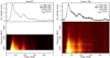 |
Fig. 1. Flux calibrated total intensity profiles made from observations made with MeerKAT (left plot) and Parkes (right plot) radio telescopes. The MeerKAT profile was made from a total of ∼32.6 h of observations with L-band receiver centred at 1284 MHz with a bandwidth of 856 MHz. The Parkes profile was made from a total of ∼14.9 h of observations with the two lower sub-bands of the UWL receiver with a centre frequency of 1536 MHz and a bandwidth of 1664 MHz. The profiles were bin-scrunched down to 512 bins across the pulse phase in order to increase the signal-to-noise ratio (S/N) per phase bin. The bottom panels show the dynamic spectra, made from 8 and 16 contiguous frequency bands for MeerKAT and Parkes, respectively. The number of bands was chosen to result in the same frequency width per band for both telescopes and correspond to the flux measurements shown in Fig. 2. The frequency range of the dynamic spectrum from MeerKAT was aligned to that of Parkes for ease of comparison. The frequency evolution of the pulse profile and the steep spectral index are clearly visible. |
3.2. MeerKAT observations
The pulsar observing set-up at MeerKAT is explained in detail by Bailes et al. (2020), while the details on polarisation and flux calibration are outlined in Serylak et al. (2021) and Spiewak et al. (2022), respectively. All timing observations were performed with the L-band receiver under two sub-themes of MeerTime: The aforementioned RelBin (Kramer et al. 2021b) and the MeerKAT census of southern MSPs (Spiewak et al. 2022). MSP census observations were short (∼5 min), while the RelBin observations ranged from 2048 s to 4 h depending upon the orbital phase, for the necessary orbital coverage. The data presented here are from March 2019 to September 2021, and amount to a total of ∼32.6 h.
The quality of the MeerKAT L-band profiles is remarkable. The timing precision, per unit time, is more than 12 times better than the earlier Parkes timing. This improvement is greater than expected given the MeerKAT’s approximately sixfold improvement in sensitivity and twofold increase in bandwidth compared to the Parkes multibeam system. The steep spectral index of the pulsar measured with the combined MeerKAT + UWL dataset (see Sect. 4.2) is a likely explanation for this disparity as the MeerKAT usable L-band frequency goes as low as 900 MHz; even its central frequency of 1284 MHz is 100 MHz lower than that of the Parkes multibeam datasets. The pulsar’s pulse profile with the MeerKAT L-band receiver is presented in Fig. 1.
4. Profile analysis
In this section we report our analysis of the pulsar’s flux density, spectral index, polarisation, and pulse broadening due to interstellar scattering using the Parkes UWL and MeerKAT L-band datasets. Unless otherwise specified, all the analyses were performed on the integrated profile obtained by summing up all the observations of the pulsar per backend. This includes a total of 32.6 h and 14.9 h for MeerKAT L-band and Parkes UWL data, respectively.
4.1. Flux density spectrum
The flux density calibration of the Parkes UWL receiver was performed using observations of the Hydra A radio galaxy as well as standard pulsar reference pointings utilising pulsed source of noise (i.e. noise diode) in the ULW receiver. In the next step, a standard flux calibration technique utilising a combination of PSRCHIVE programs (i.e. FLUXCAL and PAC) was performed as described in detail in van Straten et al. (2012). We decided to divide the observing bands of both telescopes such that the fractional per-band frequency would be the same, thus simplifying the fitting procedure. In order to estimate the flux densities for each frequency band we created an analytical pulse profile using the PAAS program. Subsequently the PSRFLUX program from the same package was used to cross-correlate it with each band’s profile. The uncertainties of flux densities in each of the frequency bands were estimated by an algorithm that robustly estimates the off-pulse baseline and is part of the PSRCHIVE package. The flux density measurements of MeerKAT data was obtained using a scaling relation from the radiometer equation as explained in Spiewak et al. (2022).
Figure 2 presents flux density measurements made with both telescopes, as well as the best fit of a power-law model, S = S1400 (ν/1400 MHz)α. The flux density spectrum of the MeerKAT L-band data (Fig. 2) is found to be well fit by a steep spectral index, α of −3.13 ± 0.02, providing a mean flux density of 0.53 ± 0.01 mJy at 1400 MHz. We note that in the region where data points from MeerKAT and Parkes UWL overlap, a slight offset between the points can be seen, with MeerKAT data points being slightly above those of Parkes UWL. We deduce this is due to the MeerKAT antenna system temperature that was assumed in the flux density measurement method mentioned above and to the varying number of antennas used per observation that were integrated into the average profile used in this analysis. Additionally, we note a slight deviation from the best-fit line seen for the Parkes UWL data points extending outside frequency overlap. We conclude that this effect could be due to the PSRFLUX underestimating flux in the frequency bands where the pulsar S/N is low. This is especially seen in the frequency-resolved plot of Fig. 3 for the Parkes UWL data at frequencies above 1.6 GHz.
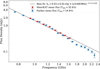 |
Fig. 2. Mean flux density measurements for the observations performed with MeerKAT L-band (red squares) and Parkes UWL (blue diamonds) receivers with error bars indicating nominal 1σ uncertainties, fit with a power-law model (black dashed line) to determine S1400 and the spectral index, α. The number of measurement points for each telescope was chosen to result in equal bandwidth. |
4.2. Polarisation properties
Figure 3 presents a flux- and polarisation-calibrated average profile for PSR J0955−6150 at L-band using MeerKAT. The profile is created from integrating a total of 32.6 h and the full MeerKAT observing band (for these observations ∼775 MHz) after radio frequency interference (RFI) removal.
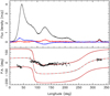 |
Fig. 3. Polarisation profile as observed with MeerKAT at a central frequency of 1284 MHz, integrating a total of 32.6 h. Top panel: total intensity (black), the linear intensity (red), and the circular polarisation intensity (blue). Bottom panel: values of the position angle (PA) swing. A RVM has been fitted to the PA values, and is shown as a red solid line and repeated offset by 180 deg, while the dashed line indicates the RVM solution separated by 90 deg and intended to fit the interpulse. The grey band indicates the derived uncertainties in the determined RVM description. See Sect. 6 for details. |
The pulsar shows a wide profile shape with broad multiple component features and a duty cycle in excess of 80% at L-band. The small-amplitude component trailing the main pulse by ∼100 deg of longitude (called a post-cursor) is not unusual for recycled pulsars, but is a typical feature that distinguishes the emission from millisecond pulsars from that of normal pulsars (Kramer et al. 1998). It may originate from the magnetic pole opposite to the one responsible for the main pulse (as it appears to be emitted in a polarisation mode orthogonal to the main pulse, cf. Sect. 6), but it may also come from a different location more generally.
The wide main pulse shows only a very small degree of polarisation, both for the linearly polarised (red) and circularly polarised (blue) component. The fact that the degree of circular polarisation exceeds that of the linear component is uncommon for a normal pulsar, but is not atypical for millisecond pulsars (Xilouris et al. 1998). In contrast, the post-cursor feature is nearly completely linearly polarised with non-detectable circular polarisation. We have calculated the phase-averaged linear polarisation fraction to be L/I = 6.2 ± 1.6%.
In the main pulse, the circular polarisation shows a sense reversal, which in normal pulsars is usually identified with the longitude of the magnetic axis (Lorimer & Kramer 2012). The phase-averaged absolute circular polarisation fraction is |V|/I = 10.2 ± 0.1%. We discuss the geometric interpretation of the polarisation properties (especially that of the position angle swing shown in the lower panel of Fig. 3) in Sect. 6.
4.3. No evidence of scattering
We investigate evidence of scattering (i.e. multipath propagation) in the interstellar medium (ISM) by fitting a pulse broadening model to the profile shapes obtained from integrating the high S/N profile to four frequency channels. From these we follow two approaches. At first the complete pulse shapes are modelled using a five-component Gaussian model (representative of the intrinsic profile) convolved with an interstellar transfer function ∝e−t/τs, where τs is the characteristic ISM scattering timescale (Williamson 1972). The Gaussian components and τs values are simultaneously fit. While we find that the channelised data are well fit by this model, as shown in Fig. 4 we observe only marginal evolution of τs with frequency; the best-fit τs values all lie between 0.02 ms and 0.03 ms using four channels across the band. The power-law scaling, τ ∝ ν−α, provides a flat α = −0.5 ± 0.5. As such α is poorly constrained and is much smaller than the value of 4 or 4.4 typically associated with simple scattering models of radio frequencies by the ionised component of the ISM (e.g. Rickett 1970, 1977). We note that for all our scattering fits there are large covariances between τs and many of the Gaussian component widths, which are used to model the underlying profile. For the lowest frequency channel in Fig. 4 the anti-correlation of τs with the three principal Gaussian component widths is > 0.8. We conclude that the obtained τs estimates are more likely a result of the profile’s asymmetric shape and its intrinsic profile evolution rather than scattering by the ISM.
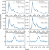 |
Fig. 4. Profiles of PSR J0955−6150 with the best fit scattering models for whole as well as post-cursor component. Top four panels: profile shapes across four MeerKAT L-band frequencies fitted with a scatter broadening model (blue dashed lines). The obtained τs values do not show significant evolution with frequency, as is typical of ISM scattering. Bottom panels: lone component isolated at phase ∼0.95, which shows a symmetric shape consistent with τs = 0. |
As a second test we investigated the isolated component (at phase 0.95) for evidence of scattering. The τs values associated with the isolated component are found to be consistent with zero (see bottom panels of Fig. 4) and are fully correlated (> 0.9) with the width of this isolated component. We conclude that we do not find evidence of pulse broadening via the ISM. We also fail to find convincing evidence for scattering in the L-band MeerKAT data of PSR J1006−6311, which has similar Galactic coordinates to PSR J0955−6150 (separated by 1.9deg in Galactic longitude and 0.3deg in latitude) and a DM of 195.99 cm−3 pc (D’Amico et al. 1998), further substantiating a lack of scattering broadening.
The NE2001 Cordes & Lazio (2002) and YMW16 Yao et al. (2017) electron density models of the Galaxy predict significantly different scattering timescales of  and
and  1; they place the pulsar at a distance of 2.17 kpc and 4.04 kpc, respectively. Comparing these estimates to the results above, we note that the NE2001 model’s results are closer to our measurements.
The lack of evidence for scatter broadening of the PSR J0955−6150 profile allows us to put limits on the intrinsic radio duty-cycle; when considering the isolated component to be the inter-pulse to this pulsar, this provides us with a duty-cycle > 95%. We can also ultimately make comparisons between its intrinsic radio and the gamma-ray emission, the latter of which is expected to have a wider pulse profile (for details, see Paper II, in prep.). Furthermore, the apparent lack of scattering makes timing of this pulsar with the MeerKAT UHF receiver even more promising.
5. Timing analysis
5.1. Data reduction
The data reduction for pulsar timing used standard pulsar timing analysis techniques using the PSRCHIVE software package (Hotan et al. 2004; van Straten et al. 2012) and all the commands and programs specified in this section are part of this package unless explicitly mentioned or cited otherwise. We used the initial AFB data ‘as is’ from the discovery paper of PSR J0955−6150 (Camilo et al. 2015). All other Parkes multibeam data were first manually mitigated of RFI using PAZI and PSRZAP and were scrunched to five-minute integrations. These were polarisation calibrated using observations of a noise diode that was performed before every pulsar observation. The noise diode injects a square wave signal cycled at 11.123 Hz at 45 degrees to each of the orthogonal signal probes. This is used to measure and compensate for the differential gain and phase that is induced across the two polarisations. The polarisation calibrated data were further scrunched such that there is one integration per observation, and two channels across the band. The data reduction for Parkes UWL was similar except that the final products had 0.7 h integrations and 13 channels across the band.
The reduction of MeerKAT data used the MEERPIPE pipeline that performs RFI excision using a modified version of COASTGUARD (Lazarus et al. 2016), performs polarisation and flux calibration, and produces decimated data products that can be readily used for timing. Depending on the observing time (which in turn depends on which Meertime ‘theme’ it belonged to, and what the orbital phase was), the final data product contained time integrations from 300 to 2048 seconds, and eight channels across the observing bandwidth.
High S/N observations were summed on a per backend basis to obtain a good frequency-resolved pulse profile. For every backend, 2D analytical templates were obtained by iteratively running the PAAS command for every channel from these high S/N profiles. The resultant analytical templates were then used to obtain frequency-resolved time of arrivals (TOAs) using the PAT command. More information on the observing system and the dataset is given in Table 2.
Details of the observing system and the timing dataset of PSR J0955−6150 used in this paper.
5.2. Timing
For the TOA analysis we used the TEMPO2 pulsar timing package (Hobbs et al. 2006) and TEMPONEST, a Bayesian parameter estimation plug-in to TEMPO2 that also facilitates fits for, among other things, power-law models for red and DM noise in the data (Lentati et al. 2014).
To describe the telescope’s motion relative to the Solar System barycentre, we used the JPL DE436 Solar System ephemeris. All ToAs were transferred to Universal Coordinated Time (UTC) and then to the terrestrial time (TT) standard that is derived from the International Atomic Time (TAI) timescale. To describe the pulsar’s orbital motion, we use two models related to the theory-independent model of Damour & Deruelle (1986) (hereafter DD). The DD model describes the orbital motion as essentially being a Keplerian orbit with small relativistic perturbations. With pulsar timing, we can only measure five of its elements: the orbital period (Pb), orbital eccentricity (e), the semi-major axis of the pulsar’s orbit projected along the ling of sight (x), the longitude of periastron (ω), and the time of passage of periastron (T0). The relativistic perturbations are quantified, in a general and theory independent way (Damour & Taylor 1992), by the so-called post-Keplerian (PK) parameters: rate of advance of periastron ( ), the variation in the orbital period (Ṗb, which includes the orbital decay caused by the emission of gravitational waves), and the Einstein delay (γ, which is caused by the orbital variation of the special relativistic time dilation and general relativistic gravitational redshift). In addition, the model includes the aforementioned Shapiro delay.
The first model we used is the DDGR orbital model, which assumes the validity of GR to describe all relativistic effects and fits directly for the masses of the two objects in the system. In parallel, we used the theory-independent orbital model (DDH) in order to understand which relativistic effects are effectively being measured; this is important for verifying whether they are all consistent with each other within the framework of GR. This model is nearly identical to the DD model. The only difference are the PK parameters used to describe the Shapiro delay: in the DD model these are the range (r) and shape (s); in the DDH model these are the orthometric amplitude (h3) and the orthometric ratio (ς, Freire & Wex 2010). The advantage of using h3 and ς is that they have, particularly for lower inclinations, a much lower correlation between themselves than r and s; therefore, they provide a better description of mass and inclination constraints introduced by the Shapiro delay. For orbital inclinations close to 90deg the two models are equivalent.
For both DDH and DDGR timing models, we performed Bayesian non-linear fits of the timing model to our data using TEMPONEST. Apart from the timing parameters, we fitted for white noise parameters (EFAC and EQUAD) per backend that modify the formal TOA uncertainties, and the power-law DM noise model described in Lentati et al. (2014). We also performed fits for a red timing noise model, but the posteriors indicated that the red noise in the dataset is negligible. Hence we ignored red timing noise for the rest of our analysis. The estimates of the pulsar parameters can be found in Tables 3 and 4; the uncertainties on the parameters represent 68.3% confidence levels that are scaled to a reduced χ2 of 1. The first table has the spin and astrometric parameters for the pulsar; the second has the binary parameters derived according to the DDGR and DDH models, and the results of our Bayesian analysis of the masses of the components using a χ2 grid, which is described in Sect. 5.6. The TOA residuals (i.e. the TOA minus the prediction of the ephemeris for that rotation) are depicted in Fig. 5. Figure 6 shows the marginalised 1D posterior distributions and the 2D correlation contours for the orbital and post-Keplerian parameters that are relevant for this paper. In the remainder of this section we note some of the timing parameters we have measured, and discuss their significance, with a special focus on the post-Keplerian parameters and the masses of the pulsar and its companion.
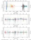 |
Fig. 5. Post-fit residuals for the timing of PSR J0955−6150, obtained with the TEMPO2 DDH solution as a function of (from top to bottom) time, orbital phase without subtracting the full Shapiro delay signal, and orbital phase after subtracting the Shapiro delay signal. The orbital phase is measured from periastron; the superior conjunction occurs at a mean anomaly of 259.9 degrees. The colours denote the different telescopes and backends used in the timing. Blue: Parkes Analogue Filterbank data, Brown and Yellow: Parkes Digital Filterbank data, Red: CASPER Parkes Swinburne Recorder data (taken both before 2017 and after 2019, thus establishing timing continuity for the whole dataset), Grey: Parkes UWL data, and Teal: MeerKAT L-band data. The middle plot also shows the theoretical Shapiro delay signal for the best value of the orbital inclination. In the bottom two plots, TOAs with precision worse than 10 μs are made semi-transparent for clarity. |
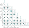 |
Fig. 6. Corner plot showing the posterior distributions of the orbital and PK parameters and the correlations between them for PSR J0955−6150 obtained from the non-linear timing of the pulsar with the DDH binary model using TEMPONEST. The off-diagonal elements show the correlation between the parameters and are marked contours that define the 39%, 86%, and 98% confidence levels, while the diagonal elements show the marginalised 1D posterior distributions of the parameters with the shaded region indicating nominal 1σ or 68.27% of the probability. |
Timing parameters for PSR J0955−6150, obtained from the TEMPO2 timing package using the DDH binary model.
Binary parameters measured for PSR J0955−6150 obtained using TEMPO2.
5.3. Position and proper motion
The timing yields a very precise position of the pulsar in the sky. This allows a search for counterparts at optical wavelengths. Inspecting the Gaia data release 3 (Gaia Collaboration 2021), we find no counterparts within 3″ of the position of the pulsar. However, this goes only to a magnitude of about 20. A deeper optical map of the southern Galactic plane has been obtained by the Cerro Tololo DECam Plane Survey (Schlafly et al. 2018), where the faintest objects have magnitudes of 23.7, 22.8, 22.3, 21.9, and 21.0 mag (AB) in the g, r, i, z, and Y bands, respectively, and an average seeing of about 1″. Again, no clear counterparts can be detected within 3″ of the position of the pulsar. In the direction of this pulsar, the extinction is 1.15, 0.773, 0.567, 0.432, and 0.376 magnitudes for the g, r, i, z, and Y bands (Schlafly & Finkbeiner 2011). This implies that the companion WD must be fainter (in the g band) than magnitude ∼21.1. This is not surprising; the WD companion of the eccentric MSP PSR J2234+0611 has a g magnitude of 22.17 (Antoniadis et al. 2016a). Furthermore, PSR J2234+0611 is at a distance 0.95 ± 0.04 kpc (Stovall et al. 2019); the estimated distance to PSR J0955−6150 is at least twice as large, which would increase its magnitude by 1.5. This means that even without extinction, the companion of PSR J2234+0611 would not be detectable at the distance of PSR J0955−6150.
We have also looked for counterparts in the near-infrared VISTA Hemisphere Survey, which has a target depth is 20.6, 19.8, and 18.5 magnitudes for the J, H, and K bands, respectively (Spiniello & Agnello 2019). Again, no clear counterparts are seen at the position of the pulsar. Thus, we cannot confirm that the companion is a He WD. If it is, it is too faint to be detectable in current surveys.
Our measurement of the proper motion of PSR J0955−6150 shows that it is unusually small, which is consistent with no detectable motion both in right ascension (α) and declination (δ); the total proper motion μ is only 0.2(1) mas yr−1. This yields a very low heliocentric velocity. If we use the NE2001 model of the electron distribution of the Galaxy (Cordes & Lazio 2002), then the distance is around 4.0(8) kpc (after assuming a distance uncertainty of about 20%) and the resulting heliocentric velocity is 3.8 ± 2.5 km s−1. Using the YMW16 model (Yao et al. 2017) we obtain a distance of 2.2(4) kpc and a heliocentric velocity of 2.0 ± 1.3 km s−1; these estimates assume only the uncertainty on the proper motion, which is, in relative terms, much larger than the uncertainty on the distance. These velocities are much lower than compared to the average velocities of MSPs (e.g. Gonzalez et al. 2011; Desvignes et al. 2016; Arzoumanian et al. 2018), and even lower than the velocities of normal pulsars (Hobbs et al. 2005).
However, the velocity of the pulsar relative to its local standard of rest is much greater. Following the simple method described by Zhu et al. (2019), we obtain peculiar velocities of ∼133 km s−1 and ∼78 km s−1 for the two distances listed above. These are nearly parallel to the Galactic plane; for instance, for the NE2001 distance the perpendicular velocity is only ∼8 km s−1. These peculiar velocity estimates are much more typical of what one finds among the general MSP population.
5.4. Spin period derivative
The proper motion measured is important for estimating the intrinsic spin-down of the pulsar, Ṗint, from the observed spin-down, Ṗobs:
 (1)
(1)
Here d is the distance from the Earth to the system, a is the difference between the acceleration of the Solar System and acceleration of the pulsar’s system in the gravitational field of the Galaxy, projected along the direction from Earth to pulsar, and c is the speed of light. The contribution to Ṗ that depends on μ is the Shklovskii effect (Shklovskii 1970); for the NE2001 distance estimate this is very small, only Pμ2d/c = 7.7 × 10⁻²⁵, a consequence of the small Heliocentric proper motion of the system.
The Galactic acceleration can be calculated using the analytical expressions in Lazaridis et al. (2009), among others; these are sufficiently accurate given the small Galactic latitude of the pulsar. In these expressions we used an estimate of the distance of the Solar System to the Galactic centre and rotational velocity of the Galaxy (D = 8.275(34) kpc, vGal = 240.5(41) km s−1) from Abuter et al. (2021). For the pulsar distance, we used the NE2001 estimate. From this, we get Pa/c = − 0.75 × 10⁻²¹.
Adding these two contributions, we obtain a total Ṗ correction Ṗk = −0.75 × 10⁻²¹, which is completely dominated by the Galactic acceleration term. From this we obtain an intrinsic spin-down of 1.501(9) × 10−20, which is similar, but slightly larger than Ṗobs. From this we estimate the characteristic age, magnetic field, and spin-down power values presented in Table 3.
5.5. Post-Keplerian parameters
As shown in Table 4, using the DDH solution, we can measure three PK parameters,  , h3, and ς, with high significance. The mass and inclination constraints that result from these parameters according to GR are depicted graphically in Fig. 7, where each triplet of lines depicts the mass and inclination constraints derived from their nominal values and 68.3% confidence level uncertainties.
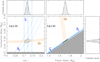 |
Fig. 7. Mass and orbital inclination constraints for the PSR J0955−6150 binary system. In both panels the lines represent the nominal and ±1σ mass and inclination constraints derived from the PK parameters of the TEMPO2 DDH solution in Table 4 (orthometric amplitude of the Shapiro delay, h3, in dashed blue; the orthometric ratio, ς, in solid blue; and the rate of advance of periastron, |

5.5.1. Rate of advance of periastron
If the rate of advance of periastron ( ) is purely relativistic, then in GR this effect yields the total mass of the system, in solar masses:
![Mathematical equation: $$ \begin{aligned} M \, = \, \frac{1}{T_\odot } \left[ \frac{\dot{\omega }}{3} (1 - e^2) \right]^{\frac{3}{2}} \left( \frac{P_{b}}{2 \pi } \right)^{5/2}. \end{aligned} $$](/articles/aa/full_html/2022/09/aa42670-21/aa42670-21-eq18.gif) (2)
(2)
Here  , with
  being the solar mass parameter (Prša et al. 2016). Since this and the speed of light c are defined exactly, the same applies to T⊙, which has a numerical value of 4.9254909476412675... μs.
The constraint on the total mass of the binary that results from  (M = 1.96(2)M⊙) is depicted graphically by the orange lines in Fig. 7. From this we obtain from Kepler’s third law an inclination-independent estimate of the orbital separation,
![Mathematical equation: $$ \begin{aligned} a = c \left[ M T_{\odot } \left( \frac{P_{b}}{2 \pi } \right)^2 \right]^{1/3} = 30.96 \, \mathrm {Gm}, \end{aligned} $$](/articles/aa/full_html/2022/09/aa42670-21/aa42670-21-eq22.gif) (3)
(3)
a value that we need below. However, for binary systems with wide orbits, the observed  might not be purely relativistic. Generally, the second most important contribution is a geometric contribution from the proper motion,
  . Re-arranging the expressions in Kopeikin (1996), we obtain
 (4)
(4)
where Θμ is the position angle of the proper motion and Ω is the position angle of the line of nodes. This expression is valid if we use the observer’s reference frame, where the position angles start from the north and increase anticlockwise through the east. In this system an orbital inclination smaller than 90 deg implies that the line-of-sight component of the orbital angular momentum points towards the Earth.
In the DDGR solution we obtain a nominal estimate of i = 83.2deg or its equally likely counterpart, 180 − i = 96.8deg. Luckily, the sign of sin i for both cases (which is what is needed in Eq. (4)) is positive. Based on this value and our current estimate of μ, the maximum value of  is ∼5 × 10⁻⁸ deg yr−1, which is uniquely small among eMSPs. This is ∼250 times smaller than the current measurement uncertainty for
  .
.
Generally, other contributions to  are very small compared to
  ; however, this is not the case in this pulsar. Using Eq. (5.17) of Damour & Schafer (1988), we find that the contribution due to the Lense–Thirring effect caused by the spin of the pulsar has a maximum value of the order of
 (5)
(5)
assuming the moment of inertia of the pulsar is 1038 kg m2. This is very similar to our current estimate of  .
.
All of this means that the observed  is purely relativistic. It also implies that an improvement in the precision of
  of two orders of magnitude will result in a similar improvement in the precision of M, which is an eventually achievable uncertainty of about 10−4 M⊙, an extraordinarily precise measurement of the mass of a MSP binary.
5.5.2. The Shapiro delay
One of the main results in this paper is the precise measurement of the Shapiro delay. This is only possible given the high timing precision achievable with MeerKAT and the high orbital inclination of about 83deg (or 180 − 83deg). In Fig. 7 we can see the mass constraints introduced, according to GR, by the two Shapiro delay parameters represented by blue lines, solid for ς and dashed for h3 (see Eqs. (22) and (23) in Freire & Wex 2010).
By itself, the Shapiro delay already yields useful mass estimates. They already characterise the WD companion as a likely He WD and the pulsar as likely massive, However, these constraints are not particularly precise. It is when this effect is combined with the the measurement of  that we obtain an order of magnitude improvement on the precision of the mass measurements. This and other results are discussed more quantitatively in Sect. 5.6.
The fact that all PK parameters cross at the same locations in the two panels of Fig. 7 constitutes a successful test of GR. However, this is not of great interest given the low precision of the masses obtained via the Shapiro delay. Instead, we can think of this multiple coincidence of PK parameters as a confirmation of the basic validity of the mass-measuring method being used, and in particular as a verification of our assertion that  is a purely relativistic effect, meaning that it has no quantifiable classical contributions, for example caused by the rotation of the companion.
5.5.3. Variation in the orbital period
For the masses determined by the DDGR model, the orbital decay caused by the emission of gravitational waves is negligible, −3.8 × 10⁻¹⁷. Much larger is the kinematic contribution to Ṗb (Ṗb,K) caused by the acceleration of the system in the gravitational field of the Galaxy (which also includes an almost negligible contribution from the Shklovskii effect). Using the same methods as those used in Sect. 5.4, we estimate Ṗb,K = −0.80 × 10⁻¹² for the NE2001 distance (d ∼ 4.0 kpc) and −0.44 × 10⁻¹² for the YMW16 distance d ∼ 2.2 kpc.
Fitting for Ṗb in the DDH model (something not done in the solution presented in Table 4), we obtain Ṗb = 9 ±6 × 10⁻¹² (68.3 % confidence level). This is 2σ consistent with the much smaller expectation for the kinematic contribution to Ṗb. This means that we have to improve the precision of Ṗb by more than one order of magnitude in order to start detecting the kinematic contribution. This is desirable since a precise measurement of the kinematic Ṗb can yield a precise distance to the system (Bell & Bailes 1996; Stairs et al. 1998); it is also achievable because the precision of the measurement of Ṗb will improve dramatically over the next few years with continued MeerKAT timing of the pulsar, particularly with the UHF receiver. However, without the TOAs from that receiver, we cannot yet simulate how long it will take until a measurement of Ṗb,K can yield a precise distance to the pulsar. Detailed simulations including the UHF data will be published elsewhere.
5.5.4. Variation in the projected semi-major axis and the Einstein delay
The proper motion also produces a secular variation in the semi-major axis. Again, re-arranging the expressions in Kopeikin (1996) and using the convention described in Sect. 5.5.1, we obtain
 (6)
(6)
which for PSR J0955−6150 yields an estimate2 of at most ± 5 × 10⁻¹⁷ lt−s s−1. Fitting for ẋ in the DDH model (something that was also not done in the solution presented in Table 4), we obtain ẋ = 4 ± 6 × 10⁻¹⁵ lt−s s−1. The uncertainty on this measurement is still ∼130 times larger than the maximum value of ẋμ.
The ẋμ is unusually small among eMSPs, partly because of the small proper motion, but also because of the high inclination. For this reason, we now estimate the future ability to measure the Einstein delay, γ.
For timing baselines that are much shorter than the precession timescale of a binary (which is certainly the case for PSR J0955−6150, where the precession timescale is  Myr), both ẋμ and γ are hopelessly correlated. The reason for this is that, under this condition, the effect of γ on the timing is merely to produce an additional secular linear contribution to the observed variation in the projected semi-major axis ẋobs, which is given by Eq. (25) of Ridolfi et al. (2019):
 (7)
(7)
For the masses in the DDGR solution in Table 4, GR predicts γ = 0.536 ms. From this, we estimate that the second term on the right-hand side is − 1.7 × 10⁻¹⁷ lt−s s−1, still twice as small as the maximum value for ẋμ. Thus, although ẋμ is exceptionally small in this system, the effect of γ in the timing is still smaller than that, and therefore γ is not independently measurable, unless the proper motion proves to be much smaller than our current estimate. This superposition with the ẋ from the proper motion prevents the measurement of γ in most eccentric wide binary pulsars, the exception being, to date, the system studied by Ridolfi et al. (2019), PSR J0514−4002A.
5.6. Bayesian mass estimates assuming GR
We now proceed to estimate the component masses and their uncertainties using a self-consistent Bayesian approach commonly used for this purpose (see e.g. Splaver et al. 2002); this is based on the quality of the TEMPO2 timing fit (measured by the resulting χ2) for the relevant physical parameters we want to measure, in this case the orbital inclination and the masses.
Because the kinematic effects on  and ẋ are not measurable, we have no information whatsoever on the line of nodes, Ω (see Sects. 5.5.1 and 5.5.2). This means that instead of mapping the χ2 for a 3D space, with axes given by Ω, cos i, and M, as in Freire et al. (2011) and Stovall et al. (2019), we can just map the cos i – M space, as done by Barr et al. (2017) and Zhu et al. (2019). The previous discussion also implies that, within this restricted parameter space, we can safely assume that GR correctly accounts for all relativistic effects; for this reason we used the DDGR orbital model to do the mapping. We refer the reader to Barr et al. (2017) for a detailed description of how the 2D probability density functions (pdfs) are derived.
For the PSR J0955−6150 system, the 2D pdfs are shown in the main panels of Fig. 7 as the closed black contours; these include 68.3 and 95.4 % of the total 2D probability, which is equivalent to the 1σ and 2σ percentiles. The 1D marginalisation of these 2D pdfs along the relevant axes are presented in the side panels of that figure.
Projecting this 2D pdf along different axes results in the mass and inclination estimates reported in the last column of Table 4, which we also list in the abstract. These are fully consistent with the DDGR estimates, although slightly less precise.
6. Geometry of PSR J0955−6150 from pulse structure data
The variation in the position angle, ψ, of the linearly polarised component (see bottom panel of Fig. 3) is often described by the rotating vector model (RVM; Radhakrishnan & Cooke 1969). The RVM describes ψ as a function of the pulse phase ϕ, depending on the magnetic inclination angle, α, and the viewing angle, ζ, which is the angle between the line-of-sight vector and the pulsar’s spin. We show its modified form as presented in Johnston & Kramer (2019)
 (8)
(8)
where the position angle ψ increases clockwise on the sky. This definition of ψ is opposite to the astronomical convention (also known as the observers convention or the PSR/IEEE convention defined in van Straten et al. 2010) in which Ψ increases anticlockwise on the sky, from north to east (cf. Damour & Taylor 1992; Everett & Weisberg 2001). Therefore, when fitting Eq. (8) to position angles measured using the astronomical convention, as in Fig. 3, we invert the sign of the numerator in Eq. (8) (see Kramer et al. 2021b for details).
In the above, ϕ0 is the pulse longitude at which ψ = ψ0 and ζ = α + β, where β is the minimum impact angle of the line of sight with respect to the magnetic axis. The additional term Δ is is defined as
where a and b are the start and end of the range of phases identified as the post-cursor and Γ is the free parameter that allows a shift in longitude (owing to a variation in either the emission height or the refractive properties of the magnetospheric plasma).
Performing a fit of Eq. (8) using the method of Johnston & Kramer (2019) to the position angle of PSR J0955−6150, as shown in Fig. 3, for Δ ≡ 0 we obtain α = 73.7 ± 0.6 deg and ζ = 77.4 ± 0.7 deg. Interestingly, the determined ϕ0 = 86.5 ± 0.1 places the fiducial plane (given by the magnetic and rotation axes and the line of sight to the observer) at a longitude where the circular polarisation shows its sense reversal, giving the geometrical interpretation of the position angle already some credibility. In the resulting solution, the post-cursors’ position angle is separated from the main pulse by an orthogonal shift of 90 deg, which is not uncommon for emission from the opposite pole (e.g. Johnston & Kramer 2019).
For binaries where the spin of the pulsar is aligned with the orbital angular momentum, in the above definition of angles, ζ ≡ i (i.e. i is defined as implemented in TEMPO or TEMPO2, see Kramer et al. 2021b for details). Our measurement of the inclination angle from timing (see Table 4) of i = 83.2 ± 0.4 deg is significantly different from the value of ζ obtained from RVM fits. Allowing Γ to obtain a non-zero value in the fit (i.e. separating the emission heights of main pulse and the post-cursor) does not improve the fit (as indicated by computing the Bayesian information criterion) and yields a very similar geometry, α = 72.4 ± 0.9 deg and ζ = 76.2 ± 0.9. The resulting Γ = −6 ± 4 deg is still consistent with no shift, and thus we assume Δ ≡ 0 in the following.
It is possible that the position angle swing of recycled pulsars is not well described by a RVM. The clear deviation of the measured position angles in the longitude range at about 100 deg may be an indication of this. There are clearly a number of average pulse profiles of recycled pulsars that are apparently difficult, or impossible, to describe with a RVM. We refer to the recent discussion in Kramer et al. (2021b) for more details. In such cases, it may be possible that the underlying magnetic field geometry may be non-dipolar (e.g. caused by sweep-back of the magnetic field lines in the compact magnetosphere of millisecond pulsars that naturally lead to large emission heights relative to the light cylinder). Alternatively, an average profile may mask underlying orthogonal jumps in the position angle that distort the measured average, as known from non-recycled pulsars (e.g. Gil & Lyne 1995). Interestingly, the deviation from the RVM fit around longitude 100 deg is indeed where the model places a transition between two orthogonal branches of the RVM. We note that the emission over a wide longitude range, especially the position angles of the nearly completely polarised post-cursor provide a significant ‘leverage arm’ that is able to constrain possible geometries very significantly, as is well known from interpulse pulsars (e.g. Johnston & Kramer 2019). Recently, despite the overall difficulty in describing the position angles of recycled pulsars with RVMs, a number of cases have been presented where the orbital inclination angle determined from RVM fits was indeed in very good agreement with the value inferred from pulsar timing (see e.g. Guo et al. 2021 and Kramer et al. 2021b). Motivated by these previous findings, and with the described caveats in mind, we investigate whether the difference between ζ and i could also be due to our assumption of spin-orbit alignment. Given the unknown nature of the binary evolution of eMSPs, it is prudent to consider the possibility that the spins are indeed not aligned. In this case, we can relate ζ and i more generally following Damour & Taylor (1992),
 (9)
(9)
where δ is the misalignment angle between the pulsar spin axis and the orbital momentum vector3. In the case of δ > 0, the pulsar spin will precess about the orbital angular momentum vector with a phase angle Φp, as has been observed for a number of relativistic double neutron star systems (see e.g. Kramer 2014). Hence,
 (10)
(10)
In our case of PSR J0955−6150, the expected precession rate, Ωgeod, will be negligible, and over the timing baseline of ∼10 years we can safely assume Φp = Φ0 = const. With this in place we perform Markov chain Monte Carlo (MCMC) fits to the position angle curve applying Eqs. (8) and (9) simultaneously. We assume i to be identical to the value determined by pulsar timing (or 180 − i deg, respectively). The posterior distributions of the model parameters are shown in Fig. 8. It is interesting to note that the posterior distribution of δ, while broad, has two clear peaks just below 10 deg and around 160 deg. In both cases (prograde and retrograde), δ differs significantly from δ = 0 or 180 deg, respectively. The first peak has a much larger amplitude. Using its location as our most likely value, we obtain δ = 6.1 deg, while if we constrain for the prograde case (0 ≤ δ ≤ 90 deg), we obtain δ > 4.8 deg with 99% confidence level. This result suggests that there could indeed be (prograde) spin-orbit misalignment in this system. We note that when inspecting the retrograde solution (90 ≤ δ ≤ 180 deg), we find the peak of the pdf as δ = 159.3 deg and δ < 160.8 deg with 99% confidence level. The ratio of the peak probability of δ for the prograde to the retrograde case is 1.59.
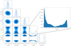 |
Fig. 8. Posterior distributions resulting from applying the RVM to the observed position angle variation, allowing for a non-zero misalignment between the spin axis and the orbital momentum vector: 0 < δ < 180 deg. |
In order to verify our method, we repeated the same procedure for PSR J1811−2405 whose original RVM fits were presented in Kramer et al. (2021b). Following a similar approach, we obtain a distribution of δ that is well in agreement of spin-orbit alignment, which means that the corresponding distribution peaks at δ = 0, as expected from circular He WD binaries. Table 5 summarises above mentioned results from applying different kinds of RVM fits to the L-band polarisation profile of PSR J0955-6150.
7. Discussion
Looking at Table 1, we see that the mass of PSR J0955−6150 is between that of PSR J1950+2414 (∼1.50 M⊙) and that of PSR J1946+3417 (∼1.83 M⊙). The NS mass distribution observed in these systems seems to be similar to that observed among MSPs in systems with He WDs in general. This is what should be expected according to both Antoniadis (2014) and Han & Li (2021). This reinforces the idea that eMSPs have a broad range of masses, which disfavours the hypotheses associated with sudden phase transitions in the interior of the MSP or its super-Chandrasekhar WD progenitor as the origin of the enhanced eccentricity. As mentioned previously, the RD-AIC hypothesis predicts that all MSPs formed that way should have a mass smaller than ∼1.3 M⊙, which is not observed. The internal phase transition theory predicts higher NS masses, but with a relatively narrow range, which is also not observed.
However, as we show below, our new measurement (0.254(2) M⊙) of the mass of the WD companion to PSR J0955−6150 independently disfavours all hypotheses suggested to date for the formation of eMSPs. The reason is that its mass is significantly lower than the predictions of Tauris & Savonije (1999) for its orbital period, and this Pb − MWD correlation is the backbone of all hypotheses for the formation of eMSPs. More specifically, using Eqs. (20) and (21) in Tauris & Savonije (1999), for an orbital period of 24.58 d the predictions for Mc vary between ∼0.271 M⊙ for Population I progenitors (corresponding to a metallicity of Z = 0.02 and independent of the initial mass of the low-mass progenitor star) and ∼0.300 M⊙ for Population II progenitors (Z = 0.001).
At first sight a WD mass deviation of the order of 0.02 M⊙ may not seem very large. However, the difference of 0.017 M⊙ relative to the lower limit of the Pb − MWD predictions, is 7.4 times larger than the measurement uncertainty. More importantly, for the observed Mc, the corresponding orbital periods are only about 14 d for Population I progenitors of the He WD and 6 d for Population II progenitors, which is a very significant deviation from the observed value of 24.58 d. A previous comparison with wide-orbit binary MSPs, although for binaries without precise mass measurements, has indicated that the Pb − MWD correlation may overestimate the WD masses (Stairs et al. 2005). The low WD mass of PSR J0955−6150 may possibly be explained by an unusually high metallicity content of its progenitor star or might be due to incorrect input physics in current modelling of the correlation. However, it is important to note that independent theoretical support for the applied Pb − MWD correlation has been provided by several more recent studies (e.g. Lin et al. 2011; Istrate et al. 2016; Soethe & Kepler 2021); see Fig. 14.14 in Tauris & van den Heuvel (2022) for an updated compilation of data.
The new result for PSR J0955−6150 is unique among eMSPs, for which previously measured He WD masses conform to the relation found by Tauris & Savonije (1999), although the companion to PSR J1946+3417 is also slightly less massive than the prediction. The small value of Mc for, in particular, PSR J0955−6150 is a highly significant result, and yet puzzling as all the suggested hypotheses naturally produce the observed range of orbital periods of eMSPs. We now look at possible explanations for this, and their implications.
7.1. Measurement precision and reliability of 
One possibility is that our measurement of  is hampered by the low quality of earlier Parkes measurements. If this is true, then future MeerKAT measurements are bound to correct this situation very quickly. Furthermore, when we exclude the earliest filterbank data (including only the more reliable coherently dedispersed data taken since June 2015), we obtain very similar masses to those reported above: Mc = 0.253(3) and Mp = 1.70(3) M⊙. Including only the high-quality MeerKAT and Parkes data taken since 2019, we obtain Mc = 0.252(3) and Mp = 1.69(3) M⊙. All these values are consistent well within their uncertainties; this means that those early data do not have a significant weight on our mass estimates, and they certainly do not bias them appreciably.
7.2. Possible mass loss from the WD
Since our mass measurement appears to be reliable, the deviation from the predictions of Tauris & Savonije (1999) is real. A possible explanation is that the mass deficiency of the companions is caused by ablation by the pulsar winds. The two systems with larger mass deficiencies, PSR J0955−6150 and J1946+3417, are associated with γ-ray emission (see Camilo et al. 2015; Smith et al. 2019). Again, this is difficult to reconcile with the fact that no significant outgassing and ablation is seen in any of the eccentric MSP+He WD systems. Such outgassing would be readily detected by the existence of eclipses and DM variations, such as those observed in many eclipsing binary pulsars. Such phenomena are not detectable in our observations of PSR J0955−6150 at any orbital phase, even at superior conjunction.
7.3. Something unique to eccentric MSPs
If mass loss from the WD cannot explain the measured low mass, we must entertain the possibility that this low mass is somehow linked to the fact that this system is an eccentric MSP. First, given the ability to measure  in these systems, we can obtain unusually precise measurements of the masses of their pulsars and He WDs. Thus, it is possible in principle that the existence of under-massive He WDs is a common occurrence among the circular MSP+He WD systems, which could have been undetected until now because of the low precision for the measurements of the masses in the vast majority of those systems. However, this is unlikely, since there is strong independent evidence that the T&S99 relation really is universal (see e.g. Tauris & van den Heuvel 2014); even the highly precise measurements for the two WDs in the triple system (Voisin et al. 2020) conform exactly to the prediction of Tauris & Savonije (1999).
Thus, we conclude the low mass of the companion to PSR J0955−6150 could be an important, but thus far hard to interpret, clue on the poorly understood formation of eMSPs. However, as discussed below, this measurement rules out current hypotheses for the formation of these systems, if one assumes that the unique orbital period–mass correlation for He WDs (Savonije 1987; Rappaport et al. 1995; Tauris & Savonije 1999; Lin et al. 2011; Istrate et al. 2016), which is based on the well-known correlation between stellar radius and degenerate core mass for low-mass giant stars (Refsdal & Weigert 1971), holds during the formation of MSP+He WD systems.
7.4. PSR J0955−6150 independently rules out phase-transition models
According to the Pb − MWD correlation from (Tauris & Savonije 1999), the companion star mass of Mc ≃ 0.254 M⊙ for PSR J0955−6150 reveals that this He WD companion must have had an orbital period between Pb, 0 = 6.19 d (Pop. II) and Pb, 0 = 14.2 d (Pop. I) at the time of its formation, depending on the chemical composition of its progenitor star (see Eqs. (20) and (21) in Tauris & Savonije 1999).
Following as an example the RD-AIC scenario, from the current pulsar mass of Mp ≃ 1.71 M⊙, we can estimate the mass of its super-Chandrasekhar mass WD progenitor, taking into account the loss of gravitational binding energy in the AIC process. The NS binding energy depends on the still somewhat uncertain equation of state. Here, we adopt the binding energy calculation from Lattimer & Yahil (1989), which as a result reveals a pre-AIC WD mass, MAIC = 1.96 M⊙, which corresponds to an instantaneous mass loss in the AIC process of about ΔM ≃ 0.246 M⊙.
Given the pre-AIC orbital period (depending on metallicity) and mass of the collapsing WD, we can calculate the post-AIC orbital parameters and compare them to those of PSR J0955−6150. The post-AIC eccentricity (assuming no kick at birth) is simply given by e = ΔM/MT (where MT = Mp + Mc), which for the derived masses yields e ≃ 0.125. This value is only marginally higher than the observed eccentricity of e = 0.1175; and adopting a slightly smaller value for the binding energy (ΔM = 0.231 M⊙) would easily reproduce the exact value of the observed eccentricity. However, the problem is to reproduce the post-AIC (present) orbital period. Assuming first a high-metallicity environment (Z = 0.02, i.e. Population I), means that the pre-AIC orbital separation was Pb, 0 = 14.2 d from the orbital period–mass correlation. For a symmetric collapse (i.e. with no kick), the change in orbital period is given by4
 (11)
(11)
such that the present (post-AIC) orbital period should be Pb = 18.4 d, which is significantly shorter than the observed value of 24.58 d. This discrepancy is only exacerbated if we assume a low-metallicity (Population II) chemical abundance of the progenitor star of the current He WD, which would then produce a post-AIC orbital period of only 8.05 d. We note that no orbital evolution of PSR J0955−6150 has taken place since its formation. The tidal torques and rate of circularization due to GR are minuscule.
To explore whether an applied momentum kick to the newborn NS could resolve the problem of reproducing the observed values of (Pb, e), we ran a number of numerical Monte Carlo simulations. We assumed the pre-AIC system was circular with an orbital period of Pb, 0 = 14.2 d (Population I star progenitor).
Figure 9 shows the results of our simulations. The open star is the pre-AIC system. The solid star is the post-AIC system for a symmetric (w = 0) AIC event. The yellow, purple, and light blue points are the outcome of AIC events with a kick velocity of w = 5, 20 and 50 km s−1, respectively, and assuming a random (isotropic) direction of the kick. The equations governing the outcome are found in Hills (1983), among others. We see that none of the simulated systems come close to the parameter space in the vicinity of PSR J0955−6150, and thus these simulations based on the RD-AIC model are not successful in explaining the formation of this eMSP.
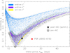 |
Fig. 9. Distribution in the (Pb, e)-plane of eMSPs simulated via the RD-AIC scenario. The red circle represents PSR J0955−6150. The black solid star is the result of a symmetric (w = 0) AIC from a 1.96 M⊙ super-Chandrasekhar WD with a pre-AIC orbital period, Pb, 0 = 14.2 d (open star), and a He WD companion star of mass Mc = 0.254 M⊙. The V-shaped coloured distributions are for the same system but applying a kick of w = 5, 20, and 50 km s−1, respectively, in a random (isotropic) direction. The grey and light grey superimposed distributions are the outcomes of simulations with more relaxed assumptions on the input physics parameters (see text). The RD-AIC scenario fails to explain PSR J0955−6150. |
To take into account the uncertainties in the gravitational binding energy for the NS, and also for the orbital period–mass correlation, we ran two extra sets of simulations where, in both cases, the pre-AIC mass (MAIC) was randomly drawn from a flat probability distribution between 1.86 − 2.06 M⊙; the pre-orbital period (Pb, 0) was randomly drawn from a flat probability distribution between 12.2 − 16.2 d; and the mass of the present He WD (Mc) was randomly drawn from a flat probability distribution between 0.251 − 0.257 M⊙. The grey and light grey points show the resultant post-AIC systems assuming randomly directed kicks of w = 20 km s−1 and w = 50 km s−1, respectively, during the AIC events. Even choosing such large AIC kicks is probably unrealistic (see e.g. Dessart et al. 2006; Gessner & Janka 2018). Nevertheless, even relaxing generously the assumed physical parameters prevents us from reproducing a system similar to PSR J0955−6150.
Therefore, we conclude that the RD-AIC hypothesis of Freire & Tauris (2014) can no longer be considered a potential model for explaining the existence of eMSPs. The RD-AIC model could explain very well the formation of the eMSPs known at that time, PSR J2234+0611 and PSR J1946+3417; however, it fails to explain PSR J0955−6150, due to its relatively low-mass He WD companion, which dictates a short orbital period that cannot be reproduced. The same arguments can be used to rule out the internal phase transition model proposed by Jiang et al. (2015) since it predicts similar constant losses in binding energy during the phase transition.
7.5. PSR J0955−6150 rules out H-shell flash models
According to Antoniadis (2014), the eMSPs were produced like regular MSP+He WD systems, which likewise follow the predictions of Tauris & Savonije (1999). Under this hypothesis, the orbital eccentricity was caused by eccentricity pumping via a circumbinary disk of material ejected by H-shell flashes in the outer layers of the proto-He WD. These H-shell flashes are likely to occur in a wide range of He WD masses between ∼0.16 and 0.32 M⊙ (depending on metallicity, Althaus et al. 2013; Istrate et al. 2016), which should then occur in the corresponding range of orbital periods observed for the eMSPs.
The expected mass loss via RLO from such vigorous thermonuclear runaway episodes is only of the order of 10−5 to 10−3 M⊙, a difference that cannot by itself explain the low mass of the companion to PSR J0955−6150. Furthermore, the ejection of such a small amount of matter is unlikely to significantly change the semi-major axis of the binary. Depending on the specific orbital angular momentum carried away by the ejected material, if anything this ejection of should actually decrease the orbit, thus bringing the new orbital period closer to the Tauris & Savonije (1999) prediction for the slightly decreased He WD mass. Thus, even after acquiring the new eccentricity, the system should retain values of Mc and Pb close to the relation predicted by Tauris & Savonije (1999).
Regarding the remaining two recent hypotheses by Han & Li (2021) related to H-shell flashes (thermonuclear rocket effect) and by Ginzburg & Chiang (2022) on resonant convection, it is not obvious that they are successful in the end. The former model has the advantage of being able to explain a broad range of eMSPs (roughly 18 − 45 d according to the authors), but the assumption of an instantaneous kick may not apply in reality. Furthermore, the predicted range of WD masses for which H-shell flashes are expected (Istrate et al. 2016) goes much beyond the narrow range of WD masses for eMSPs. The latter model has perhaps the weakness of not explaining well why some MSP binaries with orbital periods similar to those of eMSPs did not experience resonant interactions and remained in circular orbits with e ≃ 10−5 (see Fig. 1 in Stovall et al. 2019). It is also not clear whether the model can explain the offset of PSR J0955−6150 from the Pb − MWD correlation.
7.6. The misalignment angle is a potential clue to the origin of PSR J0955−6150
It is expected from binary star evolution that the spin axis of the MSP aligns with the orbital angular momentum vector as a result of mass transfer. Here we follow the arguments by Tauris & van den Heuvel (2022). During RLO, accretion torques align the spin axis of the first-born compact object (here the NS) with the orbital angular momentum vector during the recycling process (e.g. Hills 1983; Bhattacharya & van den Heuvel 1991; Biryukov & Abolmasov 2021). Observational evidence that such an alignment actually occurs in nature was given for LMXBs by Guillemot & Tauris (2014), who found agreement between the viewing angles of binary MSPs (as inferred from γ-ray light curve modelling) and their orbital inclination angles. Therefore, it is reasonable to assume δ ≃ 0 for recycled MSPs (i.e. that the MSP spin axis is at least close to parallel to the orbital angular momentum vector of the binary system).
In this work we have demonstrated for PSR J0955−6150, when assuming an ideal dipolar magnetic field, that surprisingly δ > 4.8deg. The combined unexpected result of a significant misalignment angle and this MSP being an eMSP, makes it tempting to suggest that there might be a relation between between these two circumstances. To test this idea, it is therefore important to measure (or significantly constrain) the value of δ for all other eMSP systems. In addition, we may ask which progenitor scenarios can account for such misalignment. At first sight, the thermonuclear rocket hypothesis of Han & Li (2021) may be a natural way to explain such a misalignment, if indeed the orbit is tilted as a result of thermonuclear runaway burning events (e.g. H-shell flashes).
To investigate this question, we simulated a large population of NS+ELM He WD systems similar to PSR J0955−6150 undergoing a large H-shell flash with a relatively large kick of w = 8 km s−1 (in a random direction), a large amount of ejected material of ΔM = 10−3 M⊙, and a pre-shell orbital period of Pb = 20.0 d. All systems had Mp = 1.71 M⊙ and Mc + ΔM = 0.255 M⊙ (to leave a final 0.254 M⊙ WD). The resulting misalignment angles were always δ < 4.7deg.
Even though we adopted rather large values of w and ΔM in our simulation, the thermonuclear rocket scenario of Han & Li (2021) seems to produce misalignment angles that are too small to explain the observed value of δ in PSR J0955−6150. Potentially more serious is that the assumption in this hypothesis of an instantaneous kick (compared to the timescale of Pb) is likely not justified. Assuming instead mass loss in the form of a fast wind (i.e. the Jeans mode over a timescale of several times Pb) would cause an orbital widening to only ΔPb ≃ 0.016 d, meaning that the orbit remains more or less constant with a negligible eccentricity increase.
Finally, as discussed in Sect. 7.5 and similarly to the other models discussed in this paper, there are issues with reproducing the observed orbital period for the observed WD mass in PSR J0955−6150. We therefore conclude that none of the formation hypotheses suggested in the literature to date is able to explain well the low mass of the He WD companion to PSR J0955−6150 and its orbital misalignment. This means that the formation of eMSPs remains a major puzzle of close binary stellar evolution.
8. Summary and conclusions
In this paper we have described our observations of PSR J0955−6150 with the MeerKAT and Parkes telescopes. Previously, this pulsar did not have a phase-coherent timing solution; we have reported it here for the first time. The high S/N and the resultant high-precision timing obtained with MeerKAT was instrumental for the detection and precise measurement of three PK parameters; the measurement of the rate of advance of periastron was also made possible by the large timing baseline and the fact that the system is unusually eccentric (e = 0.11) for an MSP, which makes it a member of a growing class of MSPs with He WD companions with eccentric orbits.
The measurements of these three PK parameters yielded precise mass measurements, which we discuss in light of the different hypotheses that have been advanced to explain the formation of these unusual and intriguing systems. One intriguing finding is that the He WD mass is significantly lower than predicted by current stellar evolution models. The significance of this finding is very important and could be a clue to new progress on the poorly understood formation mechanism for these eMSP systems. It is clear, however, that it independently rules out all of the proposed formation hypotheses presented to date, since in all these models the systems should obey the Pb − MWD correlation (Tauris & Savonije 1999).
Additionally, if we assume that the pulsar’s radio emission is purely dipolar where the position angle of the linear polarisation ideally follows the RVM, we find a δ > 4.8deg misalignment between the spin axis of the pulsar and the orbital angular momentum. While this result must be taken with a pinch of salt due to the not yet fully understood nature of millisecond pulsar polarisation, it is nevertheless an interesting hint that could be solidified by analysing other eMSPs. None of the formation hypotheses predict such a large misalignment, except for the thermonuclear rocket of Han & Li (2021). Assuming the assumptions behind this hypothesis to hold true, our simple toy simulation of this model indicates that the resulting misalignment angles are likely to be too small to explain the observed value of δ, although more work is needed to fully exploit this scenario. We believe that our measurement of a misalignment angle is an important datum for understanding the origin of eMSPs.
Continued observations with MeerKAT, in particular a second orbital campaign done at the UHF band, will greatly improve the precision and accuracy of the measurement of  and of the Shapiro delay as well, and allow a much improved determination of the masses of the components in this system and an improved
  –h3–ς test of GR. Continued timing will also allow a much improved measurement of Ṗb, which will eventually result in a much more precise distance to the system.
The polarimetry of the system at UHF bands, where the pulsar is much brighter, and especially a detailed study of the γ-ray emission of the system (Paper II, in prep.) have the potential to further refine our knowledge of the spin geometry of the pulsar, and confirm (or refute) our finding of the misalignment of the pulsar spin with the orbital angular momentum, which relies on the validity of the RVM model for PSR J0955−6150. Confirming this finding, preferentially in a way that is independent of the RVM, would provide a very important and unexpected datum for understanding the origin of eMSPs.
Obtained using pygedm: https://github.com/FRBs/pygedm
This is assuming the nominal value of the proper motion, which is only 1.5σ significant.
In Damour & Taylor (1992) the inclination angle is defined as iDT92 = 180 − i, which we accounted for.
See e.g. Tauris & van den Heuvel (2022).
Acknowledgments
The authors would like to thank Rosie Chen for help with analysis relating to search of the counterpart in optical and near-infrared survey data and John Antoniadis for the discussions on the evolution of the He WD companion to PSR J0955−6150. The MeerKAT telescope is operated by the South African Radio Astronomy Observatory, which is a facility of the National Research Foundation, an agency of the Department of Science and Innovation. SARAO acknowledges the ongoing advice and calibration of GPS systems by the National Metrology Institute of South Africa (NMISA) and the time space reference systems department department of the Paris Observatory. MeerTime data is housed on the OzSTAR supercomputer at Swinburne University of Technology. The Parkes radio telescope is funded by the Commonwealth of Australia for operation as a National Facility managed by CSIRO. We acknowledge the Wiradjuri people as the traditional owners of the Observatory site. This research has made extensive use of NASAs Astrophysics Data System (https://ui.adsabs.harvard.edu/) and includes archived data obtained through the CSIRO Data Access Portal (http://data.csiro.au). Parts of this research were conducted by the Australian Research Council Centre of Excellence for Gravitational Wave Discovery (OzGrav), through project number CE170100004 and the Laureate fellowship number FL150100148. VVK, PCCF, MK, AP and MCiB acknowledge continuing valuable support from the Max-Planck Society. APo and MBu acknowledge the support from the Ministero degli Affari Esteri e della Cooperazione Internazionale – Direzione Generale per la Promozione del Sistema Paese – Progetto di Grande Rilevanza ZA18GR02. MBu and APo acknowledge support through the research grant “iPeska” (PI: Andrea Possenti) funded under the INAF national call Prin-SKA/CTA approved with the Presidential Decree 70/2016. RMS acknowledges support through Australian Research Council Future Fellowship FT190100155. Pulsar research at UBC is supported by an NSERC Discovery Grant and by the Canadian Institute for Advanced Resarch. This publication made use of open source python libraries including Numpy (Harris et al. 2020), Matplotlib (Hunter 2007), Astropy (Astropy Collaboration 2018) and Chain Consumer (Hinton 2016), along with pulsar analysis packages: PSRCHIVE (Hotan et al. 2004), TEMPO2 (Hobbs et al. 2006), TEMPONEST (Lentati et al. 2014).
References
- Abuter, R., Amorim, A., & Bauböck, M. 2021, A&A, 654, A22 [NASA ADS] [CrossRef] [EDP Sciences] [Google Scholar]
- Acero, F., Ackermann, M., Ajello, M., et al. 2015, ApJS, 218, 23 [Google Scholar]
- Althaus, L. G., Miller Bertolami, M. M., & Córsico, A. H. 2013, A&A, 557, A19 [NASA ADS] [CrossRef] [EDP Sciences] [Google Scholar]
- Antoniadis, J. 2014, ApJ, 797, L24 [NASA ADS] [CrossRef] [Google Scholar]
- Antoniadis, J., Kaplan, D. L., Stovall, K., et al. 2016a, ApJ, 830, 36 [NASA ADS] [CrossRef] [Google Scholar]
- Antoniadis, J., Tauris, T. M., Ozel, F., et al. 2016b, ArXiv e-prints [arXiv:1605.01665] [Google Scholar]
- Arzoumanian, Z., Brazier, A., Burke-Spolaor, S., et al. 2018, ApJS, 235, 37 [CrossRef] [Google Scholar]
- Astropy Collaboration (Price-Whelan, A. M., et al.) 2018, AJ, 156, 123 [Google Scholar]
- Bailes, M., Jameson, A., Abbate, F., et al. 2020, PASA, 37, e028 [NASA ADS] [CrossRef] [Google Scholar]
- Barr, E. D., Champion, D. J., Kramer, M., et al. 2013, MNRAS, 435, 2234 [NASA ADS] [CrossRef] [Google Scholar]
- Barr, E. D., Freire, P. C. C., Kramer, M., et al. 2017, MNRAS, 465, 1711 [NASA ADS] [CrossRef] [Google Scholar]
- Bell, J. F., & Bailes, M. 1996, ApJ, 456, L33 [NASA ADS] [Google Scholar]
- Bhattacharya, D., & van den Heuvel, E. P. J. 1991, Phys. Rep., 203, 1 [Google Scholar]
- Biryukov, A., & Abolmasov, P. 2021, MNRAS, 505, 1775 [NASA ADS] [CrossRef] [Google Scholar]
- Camilo, F., Kerr, M., Ray, P. S., et al. 2015, ApJ, 810, 85 [NASA ADS] [CrossRef] [Google Scholar]
- Champion, D. J., Ransom, S. M., Lazarus, P., et al. 2008, Science, 320, 1309 [NASA ADS] [CrossRef] [Google Scholar]
- Cordes, J. M., & Lazio, T. J. W. 2002, ArXiv e-prints [arXiv:astro-ph/0207156] [Google Scholar]
- D’Amico, N., Stappers, B. W., Bailes, M., et al. 1998, MNRAS, 297, 28 [CrossRef] [Google Scholar]
- Damour, T., & Deruelle, N. 1986, Ann. Inst. Henri Poincaré Phys. Théor., 44, 263 [Google Scholar]
- Damour, T., & Schafer, G. 1988, Nuovo Cimento B Serie, 101, 127 [NASA ADS] [CrossRef] [Google Scholar]
- Damour, T., & Taylor, J. H. 1992, Phys. Rev. D, 45, 1840 [NASA ADS] [CrossRef] [Google Scholar]
- DeCesar, M. E., Ransom, S. M., Kaplan, D. L., Ray, P. S., & Geller, A. M. 2015, ApJ, 807, L23 [NASA ADS] [CrossRef] [Google Scholar]
- Deneva, J. S., Stovall, K., McLaughlin, M. A., et al. 2013, ApJ, 775, 51 [NASA ADS] [CrossRef] [Google Scholar]
- Dessart, L., Burrows, A., Ott, C. D., et al. 2006, ApJ, 644, 1063 [NASA ADS] [CrossRef] [Google Scholar]
- Desvignes, G., Caballero, R. N., Lentati, L., et al. 2016, MNRAS, 458, 3341 [Google Scholar]
- Edwards, R. T., & Bailes, M. 2001, ApJ, 553, 801 [NASA ADS] [CrossRef] [Google Scholar]
- Everett, J. E., & Weisberg, J. M. 2001, ApJ, 553, 341 [NASA ADS] [CrossRef] [Google Scholar]
- Freire, P. C. C., & Tauris, T. M. 2014, MNRAS, 438, L86 [NASA ADS] [CrossRef] [Google Scholar]
- Freire, P. C. C., & Wex, N. 2010, MNRAS, 409, 199 [NASA ADS] [CrossRef] [Google Scholar]
- Freire, P. C. C., Bassa, C. G., Wex, N., et al. 2011, MNRAS, 412, 2763 [NASA ADS] [CrossRef] [Google Scholar]
- Gaia Collaboration (Brown, A. G. A., et al.) 2021, A&A, 649, A1 [NASA ADS] [CrossRef] [EDP Sciences] [Google Scholar]
- Gessner, A., & Janka, H.-T. 2018, ApJ, 865, 61 [Google Scholar]
- Gil, J. A., & Lyne, A. G. 1995, MNRAS, 276, L55 [NASA ADS] [Google Scholar]
- Ginzburg, S., & Chiang, E. 2022, MNRAS, 509, L1 [Google Scholar]
- Gonzalez, M. E., Stairs, I. H., Ferdman, R. D., et al. 2011, ApJ, 743, 102 [NASA ADS] [CrossRef] [Google Scholar]
- Guillemot, L., & Tauris, T. M. 2014, MNRAS, 439, 2033 [NASA ADS] [CrossRef] [Google Scholar]
- Guo, Y. J., Freire, P. C. C., Guillemot, L., et al. 2021, A&A, 654, A16 [NASA ADS] [CrossRef] [EDP Sciences] [Google Scholar]
- Han, Q., & Li, X.-D. 2021, ApJ, 909, 161 [NASA ADS] [CrossRef] [Google Scholar]
- Harris, C. R., Millman, K. J., van der Walt, S. J., et al. 2020, Nature, 585, 357 [NASA ADS] [CrossRef] [Google Scholar]
- Hills, J. G. 1983, ApJ, 267, 322 [NASA ADS] [CrossRef] [Google Scholar]
- Hinton, S. R. 2016, J. Open Source Soft., 1, 00045 [NASA ADS] [CrossRef] [Google Scholar]
- Hobbs, G., Lorimer, D. R., Lyne, A. G., & Kramer, M. 2005, MNRAS, 360, 974 [Google Scholar]
- Hobbs, G. B., Edwards, R. T., & Manchester, R. N. 2006, MNRAS, 369, 655 [Google Scholar]
- Hobbs, G., Manchester, R. N., Dunning, A., et al. 2020, PASA, 37, e012 [NASA ADS] [CrossRef] [Google Scholar]
- Hotan, A. W., van Straten, W., & Manchester, R. N. 2004, PASA, 21, 302 [Google Scholar]
- Hunter, J. D. 2007, Comput. Sci. Eng., 9, 90 [NASA ADS] [CrossRef] [Google Scholar]
- Istrate, A. G., Marchant, P., Tauris, T. M., et al. 2016, A&A, 595, A35 [NASA ADS] [CrossRef] [EDP Sciences] [Google Scholar]
- Jiang, L., Li, X.-D., Dey, J., & Dey, M. 2015, ApJ, 807, 41 [NASA ADS] [CrossRef] [Google Scholar]
- Johnston, S., & Kramer, M. 2019, MNRAS, 490, 4565 [NASA ADS] [CrossRef] [Google Scholar]
- Jonas, J. L. 2009, IEEE Proc., 97, 1522 [Google Scholar]
- Khargharia, J., Stocke, J. T., Froning, C. S., Gopakumar, A., & Joshi, B. C. 2012, ApJ, 744, 183 [NASA ADS] [CrossRef] [Google Scholar]
- Knispel, B., Lyne, A. G., Stappers, B. W., et al. 2015, ApJ, 806, 140 [NASA ADS] [CrossRef] [Google Scholar]
- Kopeikin, S. M. 1996, ApJ, 467, L93 [NASA ADS] [CrossRef] [Google Scholar]
- Kramer, M. 2014, Int. J. Mod. Phys. D, 23, 1430004 [NASA ADS] [CrossRef] [Google Scholar]
- Kramer, M., Xilouris, K. M., Lorimer, D. R., et al. 1998, ApJ, 501, 270 [Google Scholar]
- Kramer, M., Stairs, I. H., Manchester, R. N., et al. 2021a, Phys. Rev. X, 11, 041050 [NASA ADS] [Google Scholar]
- Kramer, M., Stairs, I. H., Venkatraman Krishnan, V., et al. 2021b, MNRAS, 504, 2094 [CrossRef] [Google Scholar]
- Lattimer, J. M., & Yahil, A. 1989, ApJ, 340, 426 [NASA ADS] [CrossRef] [Google Scholar]
- Lazaridis, K., Wex, N., Jessner, A., et al. 2009, MNRAS, 400, 805 [NASA ADS] [CrossRef] [Google Scholar]
- Lazarus, P., Karuppusamy, R., Graikou, E., et al. 2016, MNRAS, 458, 868 [Google Scholar]
- Lentati, L., Alexander, P., Hobson, M. P., et al. 2014, MNRAS, 437, 3004 [NASA ADS] [CrossRef] [Google Scholar]
- Lin, J., Rappaport, S., Podsiadlowski, P., et al. 2011, ApJ, 732, 70 [NASA ADS] [CrossRef] [Google Scholar]
- Lorimer, D. R., & Kramer, M. 2012, Handbook of Pulsar Astronomy [Google Scholar]
- Lorimer, D. R., Kawash, A. M., Freire, P. C. C., et al. 2021, MNRAS, 507, 5303 [NASA ADS] [CrossRef] [Google Scholar]
- Lynch, R. S., Freire, P. C. C., Ransom, S. M., & Jacoby, B. A. 2012, ApJ, 745, 109 [NASA ADS] [CrossRef] [Google Scholar]
- Manchester, R. N., Hobbs, G., Bailes, M., et al. 2013, PASA, 30, e017 [NASA ADS] [CrossRef] [Google Scholar]
- Octau, F., Cognard, I., Guillemot, L., et al. 2018, A&A, 612, A78 [NASA ADS] [CrossRef] [EDP Sciences] [Google Scholar]
- Özel, F., & Freire, P. 2016, ARA&A, 54, 401 [Google Scholar]
- Phinney, E. S. 1992, Philos. Trans. R. Soc. London Ser. A, 341, 39 [NASA ADS] [CrossRef] [Google Scholar]
- Pijloo, J. T., Caputo, D. P., & Portegies Zwart, S. F. 2012, MNRAS, 424, 2914 [NASA ADS] [CrossRef] [Google Scholar]
- Portegies Zwart, S., van den Heuvel, E. P. J., van Leeuwen, J., & Nelemans, G. 2011, ApJ, 734, 55 [NASA ADS] [CrossRef] [Google Scholar]
- Prša, A., Harmanec, P., Torres, G., et al. 2016, AJ, 152, 41 [Google Scholar]
- Radhakrishnan, V., & Cooke, D. J. 1969, Astrophys. Lett., 3, 225 [NASA ADS] [Google Scholar]
- Rappaport, S., Podsiadlowski, P., Joss, P. C., Di Stefano, R., & Han, Z. 1995, MNRAS, 273, 731 [NASA ADS] [CrossRef] [Google Scholar]
- Ray, P. S., Abdo, A. A., Parent, D., et al. 2012, ArXiv e-prints [arXiv:1205.3089] [Google Scholar]
- Refsdal, S., & Weigert, A. 1971, A&A, 13, 367 [NASA ADS] [Google Scholar]
- Rickett, B. J. 1970, MNRAS, 150, 67 [NASA ADS] [Google Scholar]
- Rickett, B. J. 1977, ARA&A, 15, 479 [NASA ADS] [CrossRef] [Google Scholar]
- Ridolfi, A., Freire, P. C. C., Gupta, Y., & Ransom, S. M. 2019, MNRAS, 490, 3860 [NASA ADS] [CrossRef] [Google Scholar]
- Ridolfi, A., Gautam, T., Freire, P. C. C., et al. 2021, MNRAS, 504, 1407 [NASA ADS] [CrossRef] [Google Scholar]
- Savonije, G. J. 1987, Nature, 325, 416 [NASA ADS] [CrossRef] [Google Scholar]
- Schlafly, E. F., & Finkbeiner, D. P. 2011, ApJ, 737, 103 [Google Scholar]
- Schlafly, E. F., Green, G. M., Lang, D., et al. 2018, ApJS, 234, 39 [Google Scholar]
- Serylak, M., Johnston, S., Kramer, M., et al. 2021, MNRAS, 505, 4483 [NASA ADS] [CrossRef] [Google Scholar]
- Shapiro, I. I. 1964, Phys. Rev. Lett., 13, 789 [Google Scholar]
- Shklovskii, I. S. 1970, Sov. Ast., 13, 562 [Google Scholar]
- Smith, D. A., Bruel, P., Cognard, I., et al. 2019, ApJ, 871, 78 [NASA ADS] [CrossRef] [Google Scholar]
- Soethe, L. T. T., & Kepler, S. O. 2021, MNRAS, 506, 3266 [NASA ADS] [CrossRef] [Google Scholar]
- Spiewak, R., Bailes, M., Miles, M. T., et al. 2022, PASA, 39, e027 [NASA ADS] [CrossRef] [Google Scholar]
- Spiniello, C., & Agnello, A. 2019, A&A, 630, A146 [EDP Sciences] [Google Scholar]
- Splaver, E. M., Nice, D. J., Arzoumanian, Z., et al. 2002, ApJ, 581, 509 [NASA ADS] [CrossRef] [Google Scholar]
- Stairs, I. H., Arzoumanian, Z., Camilo, F., et al. 1998, ApJ, 505, 352 [NASA ADS] [CrossRef] [Google Scholar]
- Stairs, I. H., Faulkner, A. J., Lyne, A. G., et al. 2005, ApJ, 632, 1060 [NASA ADS] [CrossRef] [Google Scholar]
- Staveley-Smith, L., Wilson, W. E., Bird, T. S., et al. 1996, PASA, 13, 243 [NASA ADS] [CrossRef] [Google Scholar]
- Stovall, K., Freire, P. C. C., Chatterjee, S., et al. 2018, ApJ, 854, L22 [NASA ADS] [CrossRef] [Google Scholar]
- Stovall, K., Freire, P. C. C., Antoniadis, J., et al. 2019, ApJ, 870, 74 [NASA ADS] [CrossRef] [Google Scholar]
- Tauris, T. M., & Savonije, G. J. 1999, A&A, 350, 928 [NASA ADS] [Google Scholar]
- Tauris, T. M., & van den Heuvel, E. P. J. 2014, ApJ, 781, L13 [NASA ADS] [CrossRef] [Google Scholar]
- Tauris, T. M., & van den Heuvel, E. P. J. 2022, Physics of Binary Star Evolution (Princeton University Press) [Google Scholar]
- Tauris, T. M., Kramer, M., Freire, P. C. C., et al. 2017, ApJ, 846, 170 [Google Scholar]
- van Straten, W., Manchester, R. N., Johnston, S., & Reynolds, J. E. 2010, PASA, 27, 104 [NASA ADS] [Google Scholar]
- van Straten, W., Demorest, P., & Oslowski, S. 2012, Astron. Res. Technol., 9, 237 [NASA ADS] [Google Scholar]
- Venkatraman Krishnan, V. 2019, Ph.D. Thesis, Swinburne University of Technology [Google Scholar]
- Voisin, G., Cognard, I., Freire, P. C. C., et al. 2020, A&A, 638, A24 [NASA ADS] [CrossRef] [EDP Sciences] [Google Scholar]
- Wex, N. 2014, in Frontiers of Relativistic Celestial Mechanics, ed. S. M. Kopeikin (Berlin: de Gruyter), 2, 35 [Google Scholar]
- Williamson, I. P. 1972, MNRAS, 157, 55 [NASA ADS] [Google Scholar]
- Xilouris, K. M., Kramer, M., Jessner, A., et al. 1998, ApJ, 501, 286 [NASA ADS] [CrossRef] [Google Scholar]
- Yao, J. M., Manchester, R. N., & Wang, N. 2017, ApJ, 835, 29 [NASA ADS] [CrossRef] [Google Scholar]
- Zhu, W. W., Freire, P. C. C., Knispel, B., et al. 2019, ApJ, 881, 165 [NASA ADS] [CrossRef] [Google Scholar]
All Tables
Details of the observing system and the timing dataset of PSR J0955−6150 used in this paper.
Timing parameters for PSR J0955−6150, obtained from the TEMPO2 timing package using the DDH binary model.
All Figures
|
Fig. 1. Flux calibrated total intensity profiles made from observations made with MeerKAT (left plot) and Parkes (right plot) radio telescopes. The MeerKAT profile was made from a total of ∼32.6 h of observations with L-band receiver centred at 1284 MHz with a bandwidth of 856 MHz. The Parkes profile was made from a total of ∼14.9 h of observations with the two lower sub-bands of the UWL receiver with a centre frequency of 1536 MHz and a bandwidth of 1664 MHz. The profiles were bin-scrunched down to 512 bins across the pulse phase in order to increase the signal-to-noise ratio (S/N) per phase bin. The bottom panels show the dynamic spectra, made from 8 and 16 contiguous frequency bands for MeerKAT and Parkes, respectively. The number of bands was chosen to result in the same frequency width per band for both telescopes and correspond to the flux measurements shown in Fig. 2. The frequency range of the dynamic spectrum from MeerKAT was aligned to that of Parkes for ease of comparison. The frequency evolution of the pulse profile and the steep spectral index are clearly visible. |
| In the text | |
|
Fig. 2. Mean flux density measurements for the observations performed with MeerKAT L-band (red squares) and Parkes UWL (blue diamonds) receivers with error bars indicating nominal 1σ uncertainties, fit with a power-law model (black dashed line) to determine S1400 and the spectral index, α. The number of measurement points for each telescope was chosen to result in equal bandwidth. |
| In the text | |
|
Fig. 3. Polarisation profile as observed with MeerKAT at a central frequency of 1284 MHz, integrating a total of 32.6 h. Top panel: total intensity (black), the linear intensity (red), and the circular polarisation intensity (blue). Bottom panel: values of the position angle (PA) swing. A RVM has been fitted to the PA values, and is shown as a red solid line and repeated offset by 180 deg, while the dashed line indicates the RVM solution separated by 90 deg and intended to fit the interpulse. The grey band indicates the derived uncertainties in the determined RVM description. See Sect. 6 for details. |
| In the text | |
|
Fig. 4. Profiles of PSR J0955−6150 with the best fit scattering models for whole as well as post-cursor component. Top four panels: profile shapes across four MeerKAT L-band frequencies fitted with a scatter broadening model (blue dashed lines). The obtained τs values do not show significant evolution with frequency, as is typical of ISM scattering. Bottom panels: lone component isolated at phase ∼0.95, which shows a symmetric shape consistent with τs = 0. |
| In the text | |
|
Fig. 5. Post-fit residuals for the timing of PSR J0955−6150, obtained with the TEMPO2 DDH solution as a function of (from top to bottom) time, orbital phase without subtracting the full Shapiro delay signal, and orbital phase after subtracting the Shapiro delay signal. The orbital phase is measured from periastron; the superior conjunction occurs at a mean anomaly of 259.9 degrees. The colours denote the different telescopes and backends used in the timing. Blue: Parkes Analogue Filterbank data, Brown and Yellow: Parkes Digital Filterbank data, Red: CASPER Parkes Swinburne Recorder data (taken both before 2017 and after 2019, thus establishing timing continuity for the whole dataset), Grey: Parkes UWL data, and Teal: MeerKAT L-band data. The middle plot also shows the theoretical Shapiro delay signal for the best value of the orbital inclination. In the bottom two plots, TOAs with precision worse than 10 μs are made semi-transparent for clarity. |
| In the text | |
|
Fig. 6. Corner plot showing the posterior distributions of the orbital and PK parameters and the correlations between them for PSR J0955−6150 obtained from the non-linear timing of the pulsar with the DDH binary model using TEMPONEST. The off-diagonal elements show the correlation between the parameters and are marked contours that define the 39%, 86%, and 98% confidence levels, while the diagonal elements show the marginalised 1D posterior distributions of the parameters with the shaded region indicating nominal 1σ or 68.27% of the probability. |
| In the text | |
|
Fig. 7. Mass and orbital inclination constraints for the PSR J0955−6150 binary system. In both panels the lines represent the nominal and ±1σ mass and inclination constraints derived from the PK parameters of the TEMPO2 DDH solution in Table 4 (orthometric amplitude of the Shapiro delay, h3, in dashed blue; the orthometric ratio, ς, in solid blue; and the rate of advance of periastron, |
| In the text | |
|
Fig. 8. Posterior distributions resulting from applying the RVM to the observed position angle variation, allowing for a non-zero misalignment between the spin axis and the orbital momentum vector: 0 < δ < 180 deg. |
| In the text | |
|
Fig. 9. Distribution in the (Pb, e)-plane of eMSPs simulated via the RD-AIC scenario. The red circle represents PSR J0955−6150. The black solid star is the result of a symmetric (w = 0) AIC from a 1.96 M⊙ super-Chandrasekhar WD with a pre-AIC orbital period, Pb, 0 = 14.2 d (open star), and a He WD companion star of mass Mc = 0.254 M⊙. The V-shaped coloured distributions are for the same system but applying a kick of w = 5, 20, and 50 km s−1, respectively, in a random (isotropic) direction. The grey and light grey superimposed distributions are the outcomes of simulations with more relaxed assumptions on the input physics parameters (see text). The RD-AIC scenario fails to explain PSR J0955−6150. |
| In the text | |
Current usage metrics show cumulative count of Article Views (full-text article views including HTML views, PDF and ePub downloads, according to the available data) and Abstracts Views on Vision4Press platform.
Data correspond to usage on the plateform after 2015. The current usage metrics is available 48-96 hours after online publication and is updated daily on week days.
Initial download of the metrics may take a while.