| Issue |
A&A
Volume 652, August 2021
|
|
|---|---|---|
| Article Number | A163 | |
| Number of page(s) | 8 | |
| Section | Interstellar and circumstellar matter | |
| DOI | https://doi.org/10.1051/0004-6361/202141386 | |
| Published online | 27 August 2021 | |
Hunting the relatives of benzonitrile: Rotational spectroscopy of dicyanobenzenes★
1
Université Paris-Saclay, CNRS, Institut des Sciences Moléculaires d’Orsay,
91405
Orsay,
France
e-mail: This email address is being protected from spambots. You need JavaScript enabled to view it.
, This email address is being protected from spambots. You need JavaScript enabled to view it.
2
Department of Chemistry, Massachusetts Institute of Technology,
Cambridge,
MA
02139,
USA
3
Department of Chemistry, University of California,
Davis, One Shields Ave,
Davis,
CA
95616,
USA
4
Dipartimento di Chimica “Giacomo Ciamician”, Università di Bologna,
via F. Selmi 2,
40126
Bologna,
Italy
5
National Radio Astronomy Observatory,
Charlottesville,
VA
22903,
USA
6
Univ. Lille, CNRS, UMR 8523 – PhLAM – Physique des Lasers Atomes et Molécules,
59000
Lille,
France
Received:
26
May
2021
Accepted:
21
June
2021
Abstract
Context. The recent interstellar detections of –CN containing aromatic species, namely benzonitrile, 1-cyanonaphthalene, and 2-cyanonaphthalene, bring renewed interest in related molecules that could participate in similar reaction networks.
Aims. To enable new interstellar searches for benzonitrile derivatives, the pure rotational spectra of several related species need to be investigated in the laboratory.
Methods. We have recorded the pure rotational spectra of ortho- and meta-dicyanobenzene in the centimetre and millimetre-wave domains. Assignments were supported by high-level quantum chemical calculations. Using Markov chain Monte Carlo simulations, we also searched for evidence of these molecules towards TMC-1 using the GOTHAM survey.
Results. Accurate spectroscopic parameters are derived from the analysis of the experimental spectra, allowing for reliable predictions at temperatures of interest (i.e. 10–300 K) for astronomical searches. Our searches in TMC-1 for both ortho- and meta-isomers provide upper limits for the abundances of the species.
Key words: methods: laboratory: molecular / techniques: spectroscopic / astrochemistry / ISM: abundances / submillimeter: general
Data (FITS files) are only available at the CDS via anonymous ftp to cdsarc.u-strasbg.fr (130.79.128.5) or via http://cdsarc.u-strasbg.fr/viz-bin/cat/J/A+A/652/A163
© O. Chitarra et al. 2021
 Open Access article, published by EDP Sciences, under the terms of the Creative Commons Attribution License (https://creativecommons.org/licenses/by/4.0), which permits unrestricted use, distribution, and reproduction in any medium, provided the original work is properly cited.
1 Introduction
The recent interstellar detection of several aromatic species towards the molecular cloud TMC-1, namely benzonitrile (C6H5CN, McGuire et al. 2018), 1- and 2-cyanonaphthalenes (C10H7CN, McGuire et al. 2021), and indene (C9H8, Cernicharo et al. 2021; Burkhardt et al. 2021a), raised important questions concerning the formation pathways of such species in the interstellar medium (ISM). The establishment of benzonitrile as a convenient tracer for benzene in the ISM (Lee et al. 2019) is bringing renewed spectroscopic attention to benzene derivatives, in particular the cyano-containing species. Among these, dicyanobenzenes (hereafter, DCBs), or benzenedicarbonitriles, C6H4(CN)2, now appear as potential candidates for interstellar detection; although, to date, the lack of experimental data has prevented such searches. DCB exists under three isomeric forms: phthalonitrile (1,2-DCB or ortho-DCB), isophthalonitrile (1,3-DCB or meta-DCB), and terephthalonitrile (1,4-DCB or para-DCB). For the sake of simplicity, we adopt the o-DCB, m-DCB, and p-DCB notations in the following.
Some interest has surrounded the DCB isomers because these relatively simple derivatives of benzene enable studies regarding the influence of substitution on the structure of the phenyl ring (e.g. Schultz et al. 1986; Williamson et al. 1991; Higgins et al. 1997; Campanelli et al. 2008). Experimental investigations of DCBs have proven quite challenging, however, because of both their low solubility in common solvents and their low volatility (Barraclough et al. 1977), the latter of which has prevented gas-phase vibrational investigations so far. While the first laboratory observation of the vibrational spectra of DCBs dates back to the late 1950s (Hadden & Hamner 1959), the first vibrational assignments were only proposed in the late 1970s (Barraclough et al. 1977; Castro-Pedrozo & King 1978). These spectra have now been investigated from the infrared down to the terahertz domain (Melinger et al. 2006; Esenturk et al. 2007; Oppenheim et al. 2010). It is worth noting that some discussion surrounds the vibrational assignments, even when supported by quantum chemical calculations (Arenas et al. 1988a,b, 1989; Lopez Navarrete et al. 1993; Higgins et al. 1997; Kumar & Rao 1997; Oppenheim et al. 2010). Recently, the Raman spectrum of p-DCB has also been investigated under high pressure conditions (Li et al. 2017). Spectroscopic investigations of the electronic spectra of DCBs have been reported as well, including a few gas phase studies (e.g. Barraclough et al. 1977; Fujita et al. 1992). Of note, however, is the work of Fujita et al. (1992), which is the only report to date of a high resolution (i.e. rotationally resolved) spectrum of a DCB. The authors investigated p-DCB by laser induced fluorescence and derived rotational constants inthe ground and first excited electronic states of the species. Since p-DCB is the only DCB isomer that does not possess a permanent dipole moment, and thus cannot be measured by means of pure rotational spectroscopy, this work provides unique insights into the moments of inertia of the compound. Additionally, the derived experimental rotational constants provide a good testbed for comparison with future quantum chemical calculations.
In this paper, we report on the gas-phase investigation of the pure-rotational spectrum of the two polar DCBs, o-DCB and m-DCB (Fig. 1), in the centimetre- and millimetre-wave domains. The assignment of rotational transitions was assisted by high level quantum-chemical calculations. The line lists derived from this work enable searches for both species in the ISM. For example, in the present work, we searched the GOTHAM survey for evidence of these molecules, combining a forward modelling approach with Bayesian sampling.
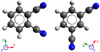 |
Fig. 1 Molecular representation of o-DCB (left panel) and m-DCB (right panel), and their principal axes of inertia. |
2 Laboratory spectroscopy
2.1 Methods
2.1.1 Samples
Powder samples of o-DCB and m-DCB (both 98% purity) were purchased from Sigma-Aldrich and used without further purification.
2.1.2 Quantum chemical calculations and spectroscopic implications
Quantum-chemical calculations were performed using Møller–Plesset second-order perturbation theory (MP2, Møller & Plesset 1934) with triple-ζ correlation-consistent polarised valence basis sets (cc-pVTZ, Dunning 1989). Geometries of o-DCB and m-DCB were optimised, yielding equilibrium rotational constants and allowing for the multipole moments (i.e. electric dipole and nitrogen quadrupole constants aswell as permanent dipole moments) to be estimated from one-electron integrals. Harmonic frequency analysis was also carried out to confirm that the optimised geometries are minimum energy structures and to estimate the value of the centrifugal distortion terms. In order to assess the accuracy of the predicted rotational constants, calculations on p-DCB were undertaken at the same level of theory (MP2/cc-pVTZ, harmonic). All the calculations were performed using Gaussian software (G16.B.01 version, Frisch et al. 2016); resulting spectroscopic parameters are reported in Table 1.
From these calculations, both o-DCB and m-DCB (Fig. 1) are shown to be planar molecules belonging to the C2v group of symmetry and possessing large permanent dipole moments, taking values of 7 and 4 Debye along the a- and b-axes of symmetry, respectively. The existence of three (for o-DCB) and two (for m-DCB) pairs of equivalent atoms with non-zero spins yields respective ortho/para ratios of 66/78 and 15/21 (see Appendix Afigure A for further details on this point).
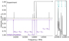 |
Fig. 2 Left panel: initial FTMW survey in search for transitions of m-DCB (upper plot in black) and comparison with a simulation of the rotational spectrum of the species using the equilibrium rotational constants and centrifugal distortion terms calculated at the MP2/cc-pVTZ level of theory (lower plot in purple, see Table 1). Dashed-red lines indicate matches between the initial prediction and the actual line position. The simulation was performed using the PGOPHER software for a rotational temperature of 2 K. The quantum numbers assignment is written in the form
|
2.1.3 Centimetre-wave spectroscopy
The pure rotational spectrum of each species has been investigated at centimetre wavelengths using a supersonic jet Fourier-transform microwave (FTMW) spectrometer located at the PhLAM Laboratory (a detailed description of the spectrometer can be found in Kassi et al. 2000; Tudorie et al. 2011). Samples were introduced in a heated reservoir located behind one of the two cavity mirrors in the high pressure region of the injection line. Similar experimental conditions were used for both o-DCB and m-DCB: samples were heated up to 413 K in the reservoir to increase their (otherwise low) vapour pressure and seeded in three bars of neon buffer gas. The mixture was subsequently injected into the FTMW chamber using gas pulses of 800 μs at a 1.5 Hz repetition rate. Rotational temperatures of about 2 K were obtained for both species. Initial surveys were performed close to the predicted frequencies of the most intense transitions expected under jet-cooled conditions (see, e.g. the left panel of Fig. 2 for m-DCB). Once the first lines were assigned, allowing an improved frequency prediction, systematic line-by-line searches for transitions in the 5–19 GHz range were undertaken.
The nuclear quadrupole hyperfine structure arising from the coupling of the total angular momentum J with the nuclear spins of the two equivalent nitrogen atoms (IN = 1) was resolved for each rotational transition under these experimental conditions. Because of the coaxial arrangement of the supersonic expansion and the cavity, each component was further split into a Doppler doublet, yielding the apparent complexity of the recorded lines (Fig. 2, right panel). The centre frequency of each transition was considered as the average of the two Doppler components, when individual structures could be deciphered (otherwise the features were not included in the fit). Resulting frequencies have an accuracy of about 2 kHz.
Experimental spectroscopic constants of o-, m-, and p-DCB; comparison with calculations at the MP2/cc-pVTZ level of theory; and parameters relevant to the fit.
2.1.4 Millimetre-wave spectroscopy
Measurements were extended at higher frequency using a (sub)millimetre spectrometer located at the ISMO laboratory (Pirali et al. 2017) for both o-DCB and m-DCB. The spectrometer consists of a radio-frequency synthesizer (Rhodes & Schwarz, SMF100A), a frequency multiplier chain from either Radiometer Physics GmbH (RPG, 75–110 GHz range) or Virginia Diodes Inc. (VDI, 140–220 GHz range), Schottky diodes for detection, and a lock-in amplifier for signal recovery. The room temperature vapour pressure of each solid sample was injected in a 2 m-long Pyrex absorption cell equipped with Teflon windows on both sides. A slow flow was ensured by a turbomolecular pump, and a pressure of 1–2 μ bar (the maximum possible under our controlled-flow conditions for these relatively low vapour pressure samples) was set in the cell. The rotational spectra of both species were acquired in the 75–110 GHz and 140–220 GHz regions, using 50 kHz frequency steps and a time constant of 100 ms. A 48.157 kHz frequency modulation with a 180 kHz or 360 kHz modulation depth – for the lower and upper frequency region, respectively – was applied to the input radiation. These modulations depth values are about twice as large as those conventionally used in these ranges, but they were chosen so as to increase the otherwise limited signal-to-noise ratio of the spectra. It is worth noting that although this procedure is made at the expanse of the full-width-at-half maximum of the transitions, the vast majority of lines remained individually resolved. Under these experimental conditions, the line centre frequency accuracy is of about 50 kHz.
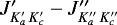
In this spectral region, the hyperfine structure of each rotational transition is unresolved. Because of the 2f modulation scheme employed on the detection side, all transitions display a second derivative line shape (Fig. 3).
 |
Fig. 3 Portions of the experimental millimetre-wave survey o-DCB (upper plots in black) and comparison with a simulation of the rotational spectrum of the species using the final best-fit constants (lower plots in bluish green, see Table 1). The PGOPHER software was used to simulate the spectrum at 300 K, the second derivative of the obtained traces was subsequently calculated to allow for a better comparison with the experimental spectrum. Additional lines present on the experimental spectrum, but not reproduced by the simulation, most likely arise from vibrational satellites (i.e. pure rotational transitions within vibrationally excited states); however, because of their lower relative intensity, no attempt was made to assign them in this work. |
2.2 Results and discussion
2.2.1 Strategy of assignment and fit
The SPFIT/SPCAT suite of programmes (Pickett 1991) was used to predict and fit the spectroscopic constants against the assigned transitions. For both o- and m-DCB species, a Watson A-reduced Hamiltonian in the Ir representation was employed (Watson 1977). All transitions were weighted according to their experimental accuracy, that is, 2 and 50 kHz for the centimetre- and millimetre-wave transitions, respectively.
A similar assignment strategy was employed for both species. Because the centimetre-wave transitions show a relatively complex hyperfine and Doppler split structure, we assigned in a first step the centre of each cluster to a virtually unsplit rotational transition (i.e. neglecting the hyperfine structure, hence using only J, Ka, Kc quantum numbers to identify energy levels), thus allowing the experimental determination of the three rotational constants A, B, and C. This significantly eased the subsequent assignment of the millimetre-wave transitions, which enabled the determination of the experimental centrifugal distortion parameters (quartics and sextics). Finally, once the full set of rotational and centrifugal distortion constants was accurately determined, the centimetre-wave transitions were reinvestigated in further detail in order to assign the individual hyperfine components, thus enabling the determination of the nuclear quadrupole coupling constants. The energy levels involved in these transitions were identified using J, Ka, Kc, I, F quantum numbers. Further information about the coupling scheme used in this work is reported in Appendix B.
Centimetre-wave transitions were assigned using the PGOPHER software (Western 2017); one of the useful features of this software is the simulation of the hyperfine structure and Doppler splitting of each transition. For the millimetre-wave transitions, the LWWa software, which allows for convenient graphical assignment using Loomis-Wood plots, was used (Lodyga et al. 2007). All experimental frequencies and fit files are provided in the CDS.
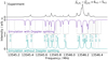 |
Fig. 4 Example of a rotational transition of o-DCB, recorded in the centimetre-wave domain using FTMW spectroscopy (black trace), showing resolved hyperfine lines, and comparison with simulations taking (in purple) and not taking (in bluish green) the Doppler splitting of each components into account (see text). Grey lines indicate the hyperfine components. Simulations were performed using the PGOPHER software and the best set of spectroscopic constants (Table 1). Quantum numbers associated with the assigned transitions are written in form I′, F′ − I″, F″. |
2.2.2 p-DCB
Because of its symmetry, the p-DCB species does not possess any pure rotational spectrum, but it can however be used to benchmark the quantum chemical calculations performed in this study. The calculated rotational constants have been compared to the experimental ones derived from jet-cooled electronic spectroscopy (Fujita et al. 1992). In the following, the agreement between experiment and theory is assessed by the percentage difference δ between experimental and calculated rotational constants, expressed as follows:
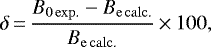 (1)
(1)
where B0 and Be denote the experimental (vibrational ground state) and calculated (equilibrium) rotational constants (A, B, or C), respectively.
At the level of theory used in this study, δ takes a value of 1% or less (Table 1). Because a similarly good agreement is expected for both o- and m-DCB, this allowed us to confidently narrow down the spectral windows for the initial searches for these species in the centimetre-wave domain.
2.2.3 o-DCB
The assignment and fit of o-DCB rotational transitions were relatively straightforward. The first rotational transitions in the centimetre-wave domain were found very close to the predictions and in total about 20 rotational transitions were assigned in this range (Fig. 4) for a total of 132 hyperfine components (105 different frequencies). In the millimetre-wave spectrum, 5635 rotational transitions were subsequently assigned to 3966 different frequencies because of unresolved asymmetric splitting for some lines.
A fit of all the assigned transitions resulted in the determination of the spectroscopic parameters presented in Table 1. The derived rotational constants are in excellent agreement with the calculated values (δ < 1%) and all the quartic and sextic centrifugal distortion constants have been determined; the predictions of the quartics show a larger deviation from the experimentally derived values, but the agreement is still very good. To account for the hyperfine structure, two nuclear quadruple coupling constants, χaa (N) and χbb (N) − χcc(N), were fitted, while χab(N) was kept fixed to its calculated value. The final standard deviation of the fit is slightly lower than 1 (0.84), which most likely reflects a conservative estimation of the line frequency uncertainties.
2.2.4 m-DCB
While the assignment of m-DCB transitions in the centimetre-wave domain was straightforward (Fig. 2), an original spectroscopic feature displayed in the millimetre-wave spectrum complicated its attribution (the rR branches display a ‘loop’, or a double band head; see Appendix C for a detailed description). As for o-DCB, all transitions were fitted together to derive a complete set of rotational spectroscopic parameters (Table 1). The same set of spectroscopic constants was adjusted, except ϕJK which was not required to fit the transitions to their experimental accuracy. Again, the standard deviation of the fit was close to unity (0.92), although slightly higher than that of o-DCB which we attribute to the lower signal-to-noise ratio of the m-DCB millimetre-wave spectrum.
2.3 Partition functions and spectral simulations at various temperatures
Most of the intense transitions at a room temperature of o-DCB and m-DCB lie in the spectral range covered by our measurements (up to 220 GHz) and they have been assigned in the present study. Frequency predictions from the derived spectroscopic constants are thus expected to be extremely reliable in this spectral region (frequency and/or quantum number extrapolation, however, can diverge rapidly). Quantitative simulations of line intensities require the use of suitable partition functions, which were determined using the SPCAT (Pickett 1991) programme and the final set of spectroscopic constants (see Appendix D for detailed values). Using these, the rotational spectra of both species can be simulated from room temperature down to a few kelvin (simulations at 8, 100, and 300 K are reported in Appendix D; the former is relevant for dark molecular clouds).
3 Astronomical searches and implications
3.1 Observations
Benzonitrile and, more recently, the naphthalene equivalents 1-cyanonaphthalene and 2-cyanonaphthalene have been detected in the cold, dark molecular cloud TMC-1 (McGuire et al. 2018, 2021). We searched for a signal from both o- and m-DCB in the same dataset from the GOTHAM (GBT Observations of TMC-1: Hunting Aromatic Molecules) project (McGuire et al. 2020). The details of the observations, dataset, and analysis procedure are provided in McGuire et al. (2021) and are only briefly summarised here. The observations were collected with the 100 m Robert C. Byrd Green Bank Telescope. The pointing centre of the observations was the ‘cyanopolyyne peak’ of TMC-1 at (J2000) α = 04h41m42.50s, δ = +25°41′26.8′′, with the pointing being checked every ~1–2 h and converging to an accuracy of ≤5′′. Observations were conducted in position-switched mode with a throw of 1° to a position verified to contain no emission.
The spectra were acquired at a native resolution of 1.4 kHz, corresponding to a velocity resolution of 0.01–0.05 kms−1 across the full bandwidth of the observations. The dataset is nearly frequency continuous from 8 to 33.5 GHz, with a gap between ~12–18 GHz. The RMS noise level varies between ~2–20 mK and is dependent on the integration time at a given frequency.
Molecules in TMC-1 tend to display four distinct velocity components, each with linewidths of ~0.1 km s−1 (Dobashi et al. 2018, 2019; McGuire et al. 2021). Typical excitation conditions within the source are Tex ~ 5–9 K. The source sizes are not well-constrained by the single-dish observations, and they are highly covariant with the derived column densities. For this reason, upper limits to the column densities of o- and m-DCB were obtained by performing Markov chain Monte Carlo (MCMC) analyses, following the procedures described in detail in Loomis et al. (2021) and McGuire et al. (2021), using the posterior parameters of benzonitrile as priors. As we are interested in determining an upper limit, the analysis performed here fixes all modelling parameters – except the four column densities – to the benzonitrile posterior means (McGuire et al. 2021).
Derived upper limit column densities for o- and m-DCB, based on MCMC simulations using the GOTHAM survey of TMC-1.
3.2 Results and implications
We detected no signal from either o- or m-DCB above 3σ significance in the GOTHAM observations of TMC-1. Upper limits to the total column densities (co-adding all four velocity components) of o- and m-DCB from our analysis are presented in Table 2. The column density of benzonitrile derived in McGuire et al. (2021) was  cm−2. Although the column density of benzene itself cannot be derived from radioastronomical observations – due to its lack of a permanent dipole moment – the most recent astrochemical models of the source suggest that benzonitrile should be a factor of ~100 lower in abundance than benzene (Burkhardt et al. 2021b).
Recent experimental work has shown the addition of a –CN group to a substituted benzene ring, toluene (C6 H5CH3), proceeds with a similar efficiency as the addition of –CN directly to benzene itself to form benzonitrile (Messinger et al. 2020). If we assume that the addition of a second –CN to benzonitrile forming o- or m-DCB is similarly efficient, an abundance ratio ~1:100 would be expected, yielding anticipated column densities of ~ 2 × 1010 cm−2. This is well below either upper limit established for the DCBs in the GOTHAM observations. From an astrochemical perspective, to date only two molecules have been detected in the ISM which contain more than one cyanide group: protonated cyanogen (NCCNH+ by Agúndez et al. 2015) and isocyanogen (NCNC; see Agúndez et al. 2018 and Vastel et al. 2019). This could be due to a lack of favourable formation routes in the ISM, simple abundance arguments, or even a lack of appropriate high-resolution spectroscopic and chemical data in support of these observations. Further study into doubly cyanated species will provide mechanistic and quantitative insight into the use of CN tagged species as polar counterparts to otherwise non-polar hydrocarbons.
4 Conclusions
In this work, we have investigated the pure rotational spectra of the two polar dicyanobenzene molecules, o- and m-DCB, from the centimetre- to the millimetre-wave domain. The spectral region covered by the present study (8–220 GHz) encompasses the strongest transitions of these molecules in the temperature range (10–100 K) most interesting for astronomical observations of the ISM. Frequency predictions using the derived set of spectroscopic constants can be used with confidence to search for the species in the ISM. While they were not detected towards TMC-1 using the GOTHAM survey data, the upper limits we derived should provide critical constraints to species containing two cyanide groups, a class of molecules that remains enigmatic in the ISM.
Acknowledgements
This project received funding from the Région Ile-de-France, through DIM-ACAV+, from the Agence Nationale de la Recherche (ANR-19-CE30-0017-01), and from the Programme National ‘Physique et Chimie du Milieu Interstellaire’ (PCMI) of CNRS/INSU with INC/INP co-funded by CEA and CNES. The authors acknowledge the use of the computing center MésoLUM of the LUMAT research federation (FR LUMAT 2764). O.C. is thankful to the ‘Groupe de Recherche’ SpecMo (GdR CNRS no. 3152) for travel support. Z.B. acknowledges support from the Chateaubriand Fellowship of the Office for Science & Technology of the Embassy of France in the United States. The National Radio Astronomy Observatory is a facility of the National Science Foundation operated under cooperative agreement by Associated Universities, Inc. The Green Bank Observatory is a facility of the National Science Foundation operated under cooperative agreement by Associated Universities, Inc.
Appendix A Statistical weight of even and odd states
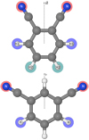 |
Fig. A.1 Molecular representation of the 1,2-dicyanobenzene (top panel) and 1,3-dicyanobenzene (bottom panel) molecules and highlight of the non-zero-spin equivalent atoms with respect to the C2v axis of symmetry. |
A.1 1,2-dicyanobenzene
The molecule has C2v symmetry and three pairs of non-zero-spin equivalent atoms that can be exchanged with respect to the C2v axis (a axis, see Fig. A.1): two pairs of H (fermions, IH = 1∕2) and one pairof N (bosons, IN = 1).
The number of symmetric wavefunctions is as follows:
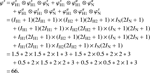 (A.1)
(A.1)
The calculation of the antisymmetric wavefunction gives φa = 78, thus an even/odd (ortho/para) states ratio of 66/78.
A.2 1,3-dicyanobenzene
The molecule has C2v symmetry and two pairs of non-zero-spin atoms that can be exchanged with respect to the C2v axis (b axis, see Fig. A.1): one pair of H (fermions, IH = 1∕2) and one pair of N (bosons, IN = 1).
The number of symmetric wavefunctions is as follows:
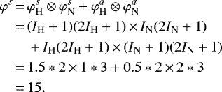 (A.2)
(A.2)
The numberof antisymmetric wavefunctions is as follows:
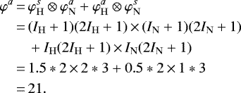 (A.3)
(A.3)
The ortho/para ratio, which is the respective weight of the even and odd states, is thus 15/21.
Appendix B Coupling scheme used
Both species studied in this work contain two identical quadrupolar nuclei, with IN = 1. The nuclear spin angular momenta are coupled as follows:

Energy levels are thus labelled using the J, Ka, Kc, I, F quantum numbers (I can take thevalues 0, 1, 2).
Since most of the observed transitions did not display any resolved hyperfine structure, for the sake of simplicity a virtual ‘dummy’ v = 1 state, sharing rotational and centrifugal distortion constants with the v = 0 (hyperfine resolved) state, was used in the fit. Within this state, only the J, Ka, Kc quantum numbers are needed to identify energy levels.
Appendix C m-DCB band loop
For m-DCB,all rR branches display a ‘loop’, or a double band head, that is, frequencies in each Ka branch increase with J, decrease, then increase again (see Fig. C.1). At first, this loop was systematically poorly predicted (the prediction of the transitions resembled that of a local perturbation), while both lower and higher J values displayed a dispersion from the prediction close to that expected for a standard branch. However, once high Ka values (above 50) were assigned in both the R- and Q-branches, which allowed for all sextic centrifugal distortion constants to be accurately determined, every loop was properly predicted and the transitions involved could readily be assigned.
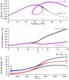 |
Fig. C.1 Illustration of the loop observed in the rR branches of m-DCB, with δ = Δ(Ka + Kc − J) = 0 ← 1; case of the rR(17) branch. For the two series of transitions, the two band heads are highlighted in orange. (top trace) Intensity of the transitions as a function of the frequency; (middle trace) transition frequency as a function of J″; and (bottom trace) reduced energy of the involved energy levels as a function of J(J + 1). Reduced energies and intensities are from an SPCAT prediction file obtained using the final set of constants (Table 1 in the main text); reduced energies were calculated using the following formula: Ereduced = E − hc × 1∕2(B + C)J(J + 1), where E is in wavenumber and B and C are in megahertz. |
Appendix D Partition function and spectral simulations at different temperatures
Partition functions (Q) of 1,2-DCB and 1,3-DCB at various temperatures.
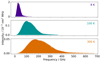 |
Fig. D.1 Spectral simulations of the rotational spectrum of 1,2-DCB at 8 K, 100 K, and 300 K performed using SPCAT, the best-fit constants, and the partitions’ functions reported in Table D.1. Similar plots are obtained for the 1,3-DCB species. |
References
- Agúndez, M., Cernicharo, J., de Vicente, P., et al. 2015, A&A, 579, L10 [NASA ADS] [CrossRef] [EDP Sciences] [Google Scholar]
- Agúndez, M., Marcelino, N., & Cernicharo, J. 2018, ApJ, 861, L22 [NASA ADS] [CrossRef] [Google Scholar]
- Arenas, J., Marcos, J., & Ramírez, F. 1988a, Spectrochim. Acta A: Mol. Spectr., 44, 1045 [Google Scholar]
- Arenas, J., Marcos, J., & Ramírez, F. 1988b, J. Mol. Struct., 175, 177 [Google Scholar]
- Arenas, J., Marcos, J., & Ramirez, F. 1989, Can. J. Spectr., 34, 7 [Google Scholar]
- Barraclough, C., Bissett, H., Pitman, P., & Thistlethwaite, P. 1977, Aust. J. Chem., 30, 753 [Google Scholar]
- Burkhardt, A. M., Lee, K. L. K., Changala, P. B., et al. 2021a, ApJ, 913, L18 [Google Scholar]
- Burkhardt, A. M., Loomis, R. A., Shingledecker, C. N., et al. 2021b, Nat. Astron., 5, 181 [Google Scholar]
- Campanelli, A. R., Domenicano, A., Ramondo, F., & Hargittai, I. 2008, J. Phys. Chem. A, 112, 10998 [Google Scholar]
- Castro-Pedrozo, M., & King, G. 1978, J. Mol. Spectr., 73, 386 [Google Scholar]
- Cernicharo, J., Agúndez, M., Cabezas, C., et al. 2021, A&A, 649, L15 [EDP Sciences] [Google Scholar]
- Dobashi, K., Shimoikura, T., Nakamura, F., et al. 2018, ApJ, 864, 82 [Google Scholar]
- Dobashi, K., Shimoikura, T., Ochiai, T., et al. 2019, ApJ, 879, 88 [Google Scholar]
- Dunning, T. H. 1989, J. Chem. Phys., 90, 1007 [Google Scholar]
- Esenturk, O., Evans, A., & Heilweil, E. J. 2007, Chem. Phys. Lett., 442, 71 [Google Scholar]
- Frisch, M. J., Trucks, G. W., Schlegel, H. B., et al. 2016, Gaussian 16, Revision B.01, Gaussian Inc. Wallingford, CT [Google Scholar]
- Fujita, K., Fujiwara, T., Matsunaga, K., et al. 1992, J. Phys. Chem., 96, 10693 [Google Scholar]
- Hadden, N., & Hamner, W. F. 1959, Analyt. Chem., 31, 1052 [Google Scholar]
- Higgins, J., Zhou, X., & Liu, R. 1997, Spectrochim. Acta A, 53, 721 [Google Scholar]
- Kassi, S., Petitprez, D., & Wlodarczak, G. 2000, J. Mol. Struct., 517, 375 [Google Scholar]
- Kumar, A., & Rao, G. 1997, Spectrochim. Acta A, 53, 2033 [Google Scholar]
- Lee, K. L. K., McGuire, B. A., & McCarthy, M. C. 2019, Phys. Chem. Chem. Phys., 21, 2946 [Google Scholar]
- Li, D., Zhang, K., Song, M., et al. 2017, Spectrochim. Acta A, 173, 376 [Google Scholar]
- Lodyga, W., Kreglewski, M., Pracna, P., & Urban, S. 2007, J. Mol. Spectr., 243, 182 [Google Scholar]
- Loomis, R. A., Burkhardt, A. M., Shingledecker, C. N., et al. 2021, Nat. Astron., 5, 188 [Google Scholar]
- Lopez Navarrete, J. T., Quirante, J. J., Aranda, M. A. G., Hernandez, V., & Ramirez, F. J. 1993, J. Phys. Chem., 97, 10561 [Google Scholar]
- McGuire, B. A., Burkhardt, A. M., Kalenskii, S., et al. 2018, Science, 359, 202 [Google Scholar]
- McGuire, B. A., Burkhardt, A. M., Loomis, R. A., et al. 2020, ApJ, 900, L10 [Google Scholar]
- McGuire, B. A., Loomis, R. A., Burkhardt, A. M., et al. 2021, Science, 371, 1265 [Google Scholar]
- Melinger, J. S., Laman, N., Harsha, S. S., & Grischkowsky, D. 2006, Appl. Phys. Lett., 89, 251110 [Google Scholar]
- Messinger, J. P., Gupta, D., Cooke, I. R., Okumura, M., & Sims, I. R. 2020, J. Phys. Chem. A, 124, 7950 [Google Scholar]
- Møller, C., & Plesset, M. S. 1934, Phys. Rev., 46, 618 [Google Scholar]
- Oppenheim, K. C., Korter, T. M., Melinger, J. S., & Grischkowsky, D. 2010, J. Phys. Chem. A, 114, 12513 [Google Scholar]
- Pickett, H. M. 1991, J. Mol. Spectr., 148, 371 [Google Scholar]
- Pirali, O., Goubet, M., Boudon, V., et al. 2017, J. Mol. Struct., 338, 6 [Google Scholar]
- Schultz, G., Brunvoll, J., & Almenningen, A. 1986, Acta Chem. Scand. A, 40, 77 [Google Scholar]
- Tudorie, M., Coudert, L. H., Huet, T. R., Jegouso, D., & Sedes, G. 2011, J. Chem. Phys., 134 [Google Scholar]
- Vastel, C., Loison, J. C., Wakelam, V., & Lefloch, B. 2019, A&A, 625, A91 [Google Scholar]
- Watson, J. K. 1977, J. Mol. Spectr., 65, 123 [Google Scholar]
- Western, C. M. 2017, J. Quant. Spectr. Rad. Transf., 186, 221 [Google Scholar]
- Williamson, B. E., VanCott, T. C., Rose, J. L., et al. 1991, J. Phys. Chem., 95, 6835 [Google Scholar]
All Tables
Experimental spectroscopic constants of o-, m-, and p-DCB; comparison with calculations at the MP2/cc-pVTZ level of theory; and parameters relevant to the fit.
Derived upper limit column densities for o- and m-DCB, based on MCMC simulations using the GOTHAM survey of TMC-1.
All Figures
|
Fig. 1 Molecular representation of o-DCB (left panel) and m-DCB (right panel), and their principal axes of inertia. |
| In the text | |
|
Fig. 2 Left panel: initial FTMW survey in search for transitions of m-DCB (upper plot in black) and comparison with a simulation of the rotational spectrum of the species using the equilibrium rotational constants and centrifugal distortion terms calculated at the MP2/cc-pVTZ level of theory (lower plot in purple, see Table 1). Dashed-red lines indicate matches between the initial prediction and the actual line position. The simulation was performed using the PGOPHER software for a rotational temperature of 2 K. The quantum numbers assignment is written in the form
|
| In the text | |
|
Fig. 3 Portions of the experimental millimetre-wave survey o-DCB (upper plots in black) and comparison with a simulation of the rotational spectrum of the species using the final best-fit constants (lower plots in bluish green, see Table 1). The PGOPHER software was used to simulate the spectrum at 300 K, the second derivative of the obtained traces was subsequently calculated to allow for a better comparison with the experimental spectrum. Additional lines present on the experimental spectrum, but not reproduced by the simulation, most likely arise from vibrational satellites (i.e. pure rotational transitions within vibrationally excited states); however, because of their lower relative intensity, no attempt was made to assign them in this work. |
| In the text | |
|
Fig. 4 Example of a rotational transition of o-DCB, recorded in the centimetre-wave domain using FTMW spectroscopy (black trace), showing resolved hyperfine lines, and comparison with simulations taking (in purple) and not taking (in bluish green) the Doppler splitting of each components into account (see text). Grey lines indicate the hyperfine components. Simulations were performed using the PGOPHER software and the best set of spectroscopic constants (Table 1). Quantum numbers associated with the assigned transitions are written in form I′, F′ − I″, F″. |
| In the text | |
|
Fig. A.1 Molecular representation of the 1,2-dicyanobenzene (top panel) and 1,3-dicyanobenzene (bottom panel) molecules and highlight of the non-zero-spin equivalent atoms with respect to the C2v axis of symmetry. |
| In the text | |
|
Fig. C.1 Illustration of the loop observed in the rR branches of m-DCB, with δ = Δ(Ka + Kc − J) = 0 ← 1; case of the rR(17) branch. For the two series of transitions, the two band heads are highlighted in orange. (top trace) Intensity of the transitions as a function of the frequency; (middle trace) transition frequency as a function of J″; and (bottom trace) reduced energy of the involved energy levels as a function of J(J + 1). Reduced energies and intensities are from an SPCAT prediction file obtained using the final set of constants (Table 1 in the main text); reduced energies were calculated using the following formula: Ereduced = E − hc × 1∕2(B + C)J(J + 1), where E is in wavenumber and B and C are in megahertz. |
| In the text | |
|
Fig. D.1 Spectral simulations of the rotational spectrum of 1,2-DCB at 8 K, 100 K, and 300 K performed using SPCAT, the best-fit constants, and the partitions’ functions reported in Table D.1. Similar plots are obtained for the 1,3-DCB species. |
| In the text | |
Current usage metrics show cumulative count of Article Views (full-text article views including HTML views, PDF and ePub downloads, according to the available data) and Abstracts Views on Vision4Press platform.
Data correspond to usage on the plateform after 2015. The current usage metrics is available 48-96 hours after online publication and is updated daily on week days.
Initial download of the metrics may take a while.