| Issue |
A&A
Volume 654, October 2021
|
|
|---|---|---|
| Article Number | A53 | |
| Number of page(s) | 13 | |
| Section | Galactic structure, stellar clusters and populations | |
| DOI | https://doi.org/10.1051/0004-6361/202141299 | |
| Published online | 08 October 2021 | |
Bound mass of Dehnen models with a centrally peaked star formation efficiency
1
Energetic Cosmos Laboratory, Nazarbayev University, 53 Kabanbay Batyr ave., 010000 Nur-sultan, Kazakhstan
e-mail: This email address is being protected from spambots. You need JavaScript enabled to view it.
2
Fesenkov Astrophysical Institute, 23 Observatory str., 050020 Almaty, Kazakhstan
e-mail: This email address is being protected from spambots. You need JavaScript enabled to view it.
3
Al-Farabi Kazakh National University, 71 Al-Farabi ave., 050040 Almaty, Kazakhstan
4
Main Astronomical Observatory, National Academy of Sciences of Ukraine, 27 Akademika Zabolotnoho St., 03143 Kyiv, Ukraine
5
Institute of Astronomy, Russian Academy of Sciences (INASAN), 48 Pyatnitskaya str., 119017 Moscow, Russian Federation
6
Rudolf Peierls Center for Theoretical Physics, University of Oxford, Parks Road, Oxford OX1 3PU, UK
7
Ratbay Myrzakulov Eurasian International Centre for Theoretical Physics, 010009 Nur-Sultan, Kazakhstan
8
Center for Theoretical Physics, Eurasian National University, 010008 Nur-Sultan, Kazakhstan
9
Physics Department, Nazarbayev University, 53 Kabanbay Batyr ave., 010000 Nur-sultan, Kazakhstan
10
Helmholtz-Institut für Strahlen- und Kernphysik, Nussallee 14-16, 53115 Bonn, Germany
11
Argelander-Institut für Astronomie, Auf dem Hügel 71, 53121 Bonn, Germany
12
National Astronomical Observatories and Key Laboratory of Computational Astrophysics, Chinese Academy of Sciences, 20A Datun Rd., Chaoyang District, Beijing 100101, PR China
13
Astronomisches Rechen-Institut am Zentrum für Astronomie der Universität Heidelberg, Mönchhofstrasse 12-14, 69120 Heidelberg, Germany
14
Kavli Institute for Astronomy and Astrophysics at Peking University, 5 Yiheyuan Rd., Haidian District, 100871 Beijing, PR China
Received:
12
May
2021
Accepted:
16
July
2021
Abstract
Context. Understanding the formation of bound star clusters with a low star formation efficiency (SFE) is important for improving our knowledge of the star-formation history of galaxies. In N-body models of star-cluster evolution after gas expulsion, the Plummer model with an outer power law density profile has been used in a broad range of studies.
Aims. Here, we study the impact of the density profile slopes on the survivability of the low-SFE star clusters after instantaneous gas expulsion. We compare cases when a stellar cluster exhibits a Plummer profile to those with Dehnen profiles, including cuspy ones of different slopes at the time of formation.
Methods. We determined the corresponding density profile of the residual gas for a given global SFE, assuming that our model clusters formed with a constant efficiency per free-fall time and, hence, with a shallower density profile for the gas than that of the stars. We performed direct N-body simulations of evolution of clusters initially in virial equilibrium within the gas potential following gas removal.
Results. We find that the violent relaxation lasts no longer than 20 Myr, independently of the density profile power law slopes. Dehnen model clusters survive after violent relaxation with significantly lower SFEs when the global SFE measured within the Jacobi radius or within a half-mass radius. Dehnen γ = 0 model clusters show a similar final bound fraction with the Plummer model clusters if the global SFE is measured within ten scale radii. The final bound fraction increases with the γ values for a given global SFE.
Conclusions. We conclude that Dehnen clusters better resist the consequences of the violent relaxation that follows the instantaneous gas expulsion, as compared to the Plummer clusters. Therefore, the shallower the outer density slope of the low-SFE clusters, the better their prospects for survival after gas expulsion. Among the Dehnen clusters, we find that the steeper the inner slope, the higher the bound mass fraction that is retained, following the violent relaxation for a given global SFE.
Key words: open clusters and associations: general / galaxies: star clusters: general / stars: kinematics and dynamics / methods: numerical
© ESO 2021
1. Introduction
Star clusters form in dense gas clumps within molecular clouds (Krumholz et al. 2019; Krause et al. 2020). The stellar feedback from the newly born massive stars cleans up the star-formation region, removing the residual gas within a short timescale prior to the first supernova explosion (SNe; Kruijssen et al. 2019). The velocity of the stellar feedback has been estimated to be about 10 km s−1, both based on theory and the observations (Rahner et al. 2019; Grasha et al. 2019). All clusters older than 10 Myr are observed to be gas-free (Lada & Lada 2003; Leisawitz et al. 1989). Lada & Lada (2003) concluded that only about ten percent of the newly formed clusters survive the gas expulsion. These authors proposed that most of clusters dissolve early as a consequence of gas expulsion because of their low star-formation efficiency (SFE). Krumholz et al. (2019) attributes this to the 90 percent weight-loss on the part of star clusters, rather than to the early dissolution of most clusters.
The SFE is the fraction of star-forming gas mass converted into stars, which is measured in observed star-forming regions and found to barely reach 30 percent, and remains mostly below 20 percent (Higuchi et al. 2009; Murray 2011; Kainulainen et al. 2014). On the Galactic scale, SFE integrated throughout several star-forming regions remain at the level of about a few percent (Kruijssen et al. 2019). A large number of works have been dedicated to studying how star clusters survive after gas expulsion and the subsequent violent relaxation (Tutukov 1978; Hills 1980; Lada et al. 1984; Verschueren & David 1989; Adams 2000; Goodwin & Bastian 2006; Baumgardt & Kroupa 2007; Smith et al. 2011; Lee & Goodwin 2016; Shukirgaliyev et al. 2017; Brinkmann et al. 2017; Farias et al. 2018, and many others). Baumgardt & Kroupa (2007) showed that clusters can survive with small SFEs, namely, at about 10–15 percent, if the residual gas is expelled gradually within several crossing times. Summarizing the preceding N-body simulations, they reported that the minimum of 30 percent of star-forming gas should be converted into stars to survive the instantaneous gas expulsion as a bound cluster. By SFE, we are referring to the “total” SFE:
 (1)
(1)
where M⋆ is the total mass of stars formed in the clump before gas expulsion, Mgas is the residual gas mass at the time of gas expulsion, and the total initial mass of the star-forming clump is M0 = M⋆ + Mgas.
Baumgardt & Kroupa (2007) considered the Plummer model (Plummer 1911) star clusters in virial equilibrium within the total gravitational potential of stars and residual gas immediately before gas expulsion. The density profiles of stars and gas have the same shapes, namely, Plummer profiles with the same scale radius, aP, but different masses, in their study. Therefore, the SFE is radially constant within their model embedded clusters. Here, we introduce the form of the Plummer profile for the sake of clarity:
 (2)
(2)
Goodwin & Bastian (2006) (see also Goodwin 2009) introduced the effective SFE (eSFE), defined based on the dynamical state of the cluster immediately after gas expulsion:
 (3)
(3)
Here, the virial ratio, Q, is the ratio of the total stellar kinetic energy, K, to the absolute value of the total stellar potential energy, W,
 (4)
(4)
and the virial equilibrium is defined at Q = 1/2. They concluded that star clusters can survive instantaneous gas expulsion if eSFE > 0.30. In the model clusters of Baumgardt & Kroupa (2007), the eSFE is equivalent to the total SFE, because gas and stars follow the same density profile and stars are in virial equilibrium in the total gravitational potential. However, the eSFE can be different from the total SFE, depending on the cluster virial state prior to the gas expulsion (Goodwin 2009; Lee & Goodwin 2016). Furthermore, Goodwin (2009) discussed the survivability of star clusters that are not in virial equilibrium within the total gravitational potential of stars and gas before the gas expulsion. If the gas-embedded clusters are sub-virial (i.e., 2K < |W|) before the gas expulsion, then their eSFE can be larger than their total SFE and they may thus survive the instantaneous gas expulsion with a low total SFE (Verschueren & David 1989; Verschueren 1990; Lee & Goodwin 2016; Li et al. 2019).
Adams (2000) showed, semi-analytically, that low-SFE clusters can survive instantaneous gas expulsion if the density profile of stars has a steeper outer slope than that of the residual gas. In this case, the local SFE (SFEloc(r)) – SFE measured locally at arbitrary location within the cluster is not radially constant. We can define the SFEloc(r) as the ratio of the stellar density to the total density within a given region:
 (5)
(5)
where ρ⋆(r), ρgas(r) and ρ0(r) are local density of stars, unprocessed gas and the total initial starless gas, respectively. The cumulative SFE:
 (6)
(6)
also varies radially, decreasing with radius, since the cumulative mass of the residual gas grows faster with radius than that of stars. This is especially valid in the case of Adams (2000), where the residual gas density is ρgas ∝ r−2, with the SFEr(r) continuously decreasing with radius because the residual gas mass diverges. Therefore, Adams (2000) introduced the outer truncation radius, where the stellar density, ρ⋆, goes down to zero in his models, to measure the SFE. However, depending on the density profile applied for stars, this kind of truncation radius can be as large as +∞ (e.g., for the Plummer model).
Smith et al. (2011) proposed the formation of clusters via a hierarchical merger of sub-structured clusters within different residual gas backgrounds. These authors considered cluster models with SFEtot = 0.20 where stars are distributed within fractal sub-clusters (Goodwin & Whitworth 2004) or clumpy Plummer spheres, and arbitrarily chosen different gaseous backgrounds (from the Plummer to homogeneous spheres).
Smith et al. (2011) concluded that the key parameter showing whether cluster survives the instantaneous gas expulsion is not the total SFE, but the local stellar fraction (LSF), which is the cumulative SFE measured within the half-mass radius of the stellar component of the embedded cluster, rh, at the onset of gas expulsion:
 (7)
(7)
Cluster formation through hierarchical merger of sub-clusters also appears in hydro-dynamical simulations, starting from an initially homogeneous sphere of molecular gas (e.g., Wall et al. 2019, 2020; Li et al. 2019; Grudić et al. 2021; Fukushima & Yajima 2021). However, Chen et al. (2021) recently showed that initially centrally concentrated gas clouds (i.e., with a power density profile) tend to form a massive central cluster that grows in mass through the accretion of gas around it. Additionally, they noticed that the steeper the power law density profile, the more massive the central cluster.
Shukirgaliyev et al. (2017) performed series of N-body simulations of bound cluster formation following instantaneous gas expulsion with physically motivated star-formation conditions of Parmentier & Pfalzner (2013). The local-density driven clustered star formation model, proposed by Parmentier & Pfalzner (2013), assumes that stars form in centrally-concentrated spherically-symmetric dense gas clump with a constant SFE per free-fall time (ϵff = const). Here, the free-fall time is defined as:
 (8)
(8)
where G is the gravitational constant. As a consequence, the inner dense gas produces more stars than the outer diffuse gas within a given physical time of star-formation (SF) duration, tSF. Thus stars have steeper (power law) density profile than the initial starless gas and the residual gas prior to gas expulsion (Parmentier & Pfalzner 2013; Shukirgaliyev et al. 2017).
Assuming that the Plummer star clusters formed with ϵff = const during tSF, Shukirgaliyev et al. (2017) reconstructed the corresponding density profiles of the residual gas before gas expulsion. They show that the product of ϵff × tSF determines the cluster’s global SFE. Shukirgaliyev et al. (2017) defined the global SFE in their models as the cumulative SFE measured within ten Plummer scale radii (10aP), where over 98 percent of the stellar mass resides at the time of instantaneous gas expulsion:
 (9)
(9)
They showed that their model clusters have a centrally peaked SFE-profile (see e.g., Fig. 2 of Shukirgaliyev 2018). From the results of N-body simulations, they concluded that the minimum global SFE needed to survive as a bound cluster is SFEgl = 0.15 for their model clusters, independent of the cluster stellar mass (Shukirgaliyev et al. 2018) and as well as of the impact of the Galactic tidal field (Shukirgaliyev et al. 2019, 2020).
In the observed nearby star-forming regions, the gas and stars do not follow the same density profiles. Gutermuth et al. (2011) reported on the power law correlation:
 (10)
(10)
between the local surface densities of young stellar objects, Σ⋆, and the column density of gas, Σgas, in eight nearby star-forming regions (see also the recent results of Pokhrel et al. 2020). This corresponds to an increase in SFE with increasing gas density, meaning that the stellar density profile has a steeper power law slope than that of gas. Parmentier & Pfalzner (2013) explained that such a correlation is the consequence of the star formation taking place with a constant efficiency per free-fall time with their local-density-driven clustered star-formation model. In the state-of-the-art hybrid hydro-dynamical/N-body simulations of clustered star formation, the residual gas and newly formed stars follow power law density profiles with indexes of about 2 and 3, respectively (Li et al. 2019; Fujii et al. 2021b). In fact, Parmentier & Pfalzner (2013) noticed that the outer slope of the power law density profile of the newly formed stellar cluster will be steeper by a factor of 1.5 at most than that of the initial starless gas according to their model. That is, if the initial starless gas has a power law profile of ρ0 ∝ r−p, with an index of p = 2, then stars would follow the power law profile of ρ⋆ ∝ r−q, with index of q ≤ 3p/2 = 3 (Parmentier & Pfalzner 2013). In the case of Shukirgaliyev et al. (2017) the formed cluster follows the Plummer density profile, namely, q = 5 at the outer part, and the density profile of the initial star-forming gas at the outer part follows the power law, with p ≈ 3.3. In Fig. 1, we demonstrate this relation between the slopes of power law densities for a few fiducial cases of the Plummer-like stellar density profiles  (see Eq. (2)), with q = 3, 4, 5 (for a⋆ = 1 pc and M⋆ = 6000ℳ⊙), and the initial gas power law density profiles ρ0 ∝ (1 + r2/a2)−p/2, with p = 2, 2.6, 3.3, respectively. The initial gas profile is ρ0 = ρ⋆ + ρgas(ϵfftSF), where ρgas is the recovered density profile of the residual gas after time tSF = 3 Myr since the onset of the star formation with ϵff = 0.05. The power law density slope of the observed gas clumps commonly varies in the range of 1 ≤ p ≤ 2 (Lada et al. 2010; Kainulainen et al. 2014; Parmentier & Pasquali 2020). However, Schneider et al. (2015) reported on molecular gas clumps having a steep power law density slope up to p < 4. That means that any of the three fiducial models we show in Fig. 1 may exist according to observations.
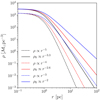 |
Fig. 1. Plummer-like power law density profiles of stellar clusters for q = 3, 4, 5, and of the corresponding initial gas, with p = 2, 2.6, 3.3. The density profiles of the initial gas were recovered according to the star cluster formation model of Parmentier & Pfalzner (2013), alike in Shukirgaliyev et al. (2017), for ϵff = 0.05, and tSF = 3 Myr. |
Almost all studies investigating the evolution of star clusters using N-body simulations consider the Plummer profile to represent the stellar density distribution before gas expulsion (Baumgardt & Kroupa 2007; Lee & Goodwin 2016; Shukirgaliyev et al. 2017). However, the commonly observed gaseous clumps have rather shallow density profiles as compared to that of the residual gas in the case of the Plummer profile (< p = 3.3). This gives rise to the question of whether it is possible that stellar clusters have shallower slope of density profile than that of the Plummer profile at the time of formation before gas expulsion. And if so, we consider how it might help in allowing such clusters to survive the instantaneous gas expulsion better than in the case of the previously considered Plummer model.
Li et al. (2019) conducted hydro-dynamical simulations followed by N-body simulations that showed star clusters with a shallow (2 < q < 3.5) power-law density profile can survive the stellar feedback driven gas expulsion with total SFEs below 10 percent. Fujii et al. (2021a), summarizing the results from their hybrid hydro-dynamical/N-body simulations of cluster formation, stated that the use of simplified models of star formation and instantaneous gas expulsion is sufficient for studying cluster mass function and the dynamical evolution of star clusters after gas expulsion. Because the hybrid hydro-dynamical/N-body simulations are expensive computationally, they can be limited to a few models or to the low-mass or low-resolution cases (Li et al. 2019). Therefore, we decided to continue studying the star cluster dynamical evolution after gas expulsion with the methods we developed in Shukirgaliyev et al. (2017). Since the Plummer model has too steep a power-law density to adequately represent the stellar component of the commonly observed embedded clusters, we propose a new set of numerical experiments using the family of the Dehnen (1993) model density profiles (with an outer slope of q = 4). The Dehnen model clusters have a shallower power density outer slope than that of the Plummer, but the former have finite mass in contrast to the case of a power density of q = 3. Also, the power-law index of density profile of the star-forming gas is expected to be p ≥ 8/3 ≈ 2.6, which is still in the range of the observed values for molecular clumps (Schneider et al. 2015).
In this work, we study the impact of the outer and inner density slopes on the survivability of star clusters after instantaneous gas expulsion. We consider the instantaneous gas expulsion, as it is the worst-case scenario for the cluster survival after gas expulsion, thus representing the lower-limit of the cluster’s survivability. The gradual gas expulsion allows clusters to keep more stars bound after violent relaxation than the instantaneous one (Geyer & Burkert 2001; Baumgardt & Kroupa 2007; Brinkmann et al. 2017). It is still unclear how the gas expulsion happens in real systems (Krumholz & Matzner 2009; Fujii et al. 2021a). Nevertheless, the gas expulsion phase, which is mostly driven by the most massive O-B stars, does not last much longer than the free-fall time of the star-forming clump (Li et al. 2019), whose results are not too different from those of the instantaneous gas expulsion (Baumgardt & Kroupa 2007). Also, since only the massive stars are responsible for gas expulsion, it is enough if a few of the most massive stars switch on their stellar wind within a short time interval in order to start driving gas out of the cluster.
In Sect. 2, we describe our Dehnen model clusters in comparison with the Plummer model case. Also we discuss measurements of the SFE with different methods and how they are done for our models. Then we present the main results in Sect. 3, namely, the bound mass evolution and the survivability of model clusters. In Sect. 4, we present a discussion and we summarize our new results.
2. Methods and models
2.1. Models of stellar cluster
We built star cluster models with different formation conditions (i.e., different SFE), where the stellar component of the embedded cluster has identical properties (e.g., mass, density profile, size). This means that the properties (e.g., density profile, mass) of the initial and the residual gas are reconstructed based on the assumption that our model clusters were formed according to the local-density-driven cluster formation model of Parmentier & Pfalzner (2013) for a given global SFE. This “upside-down” approach – as compared to Parmentier & Pfalzner (2013) – is needed for us to be able to compare star cluster models with different SFE to one another. That is to say that if we could start from a molecular clump with a given mass and size, the newly formed star clusters with different SFEs would differ also in size, mass and their density profiles. These would all make them incomparable to one another. In the other hand, this method would allow us to explore the long-term evolution of star clusters until their dissolution in the tidal field of the host galaxy, taking into account the formation conditions across a wide range of the initial conditions (see also Shukirgaliyev 2018).
Dehnen (1993) introduced the family of two-power-density spherical models. These models were originally intended to describe the spatial distributions of stars in galaxies, however, it has never been used to describe star clusters due to its large outer radius. We bring in the density profile expression of the Dehnen model here, for the sake of clarity:
 (11)
(11)
where M⋆ is the total stellar mass, aD is the Dehnen scaling radius, and γ describes the inner power-law profile of the family of Dehnen models (0 ≤ γ < 3). Figure 2 shows the comparison of these density profiles for γ = 0, 1, 2 (red, green, and blue solid lines) and the Plummer model (black dashed line) clusters, while Fig. 3 demonstrates their cumulative mass distributions. We assume that these clusters have identical stellar mass, M⋆, and half-mass radius, rh. Since we equate masses and half-mass radii of the our model clusters, their scale radii become different from each other (see vertical lines in Fig. 2). The relations between half-mass and scale radii for the Dehnen and the Plummer models are given below:
 (12)
(12)
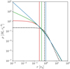 |
Fig. 2. Volume density profiles of star clusters with equal masses and half-mass radii corresponding to the Dehnen models (γ = 0, 1, 2 in red, green and blue solid lines, respectively), and the Plummer model (black dashed line). The vertical lines show the corresponding scale radii, aD and aP with respective colors. |
and
 (13)
(13)
The units of distance and mass in Fig. 2 are normalized to the cluster half-mass radius and stellar mass, thus densities are presented in the corresponding units of ![Mathematical equation: $ \left[M_\star r_\mathrm{h}^{-3}\right] $](/articles/aa/full_html/2021/10/aa41299-21/aa41299-21-eq15.gif) . We note that for equal scale radii, the central densities of the Dehnen γ = 0 and the Plummer models are equal, but then their half-mass radii would be different. The half-mass radius is used to describe the cluster size in the majority of star cluster studies. Therefore, to remain consistent with them, we also chose the half-mass radius of star clusters to represent their sizes. In the Dehnen models, the transition from the inner power-law to the outer power-law is smoother compared to that of the Plummer model. From Fig. 3 we can see that the Dehnen model clusters contain about 90 percent of their mass within the sphere of radius larger than 10rh. The Plummer model is quite compact in this sense and reaches up to 90 percent of its mass already within 3rh. However, it should be noted that the Dehnen clusters have a more compact and denser core than the Plummer cluster.
. We note that for equal scale radii, the central densities of the Dehnen γ = 0 and the Plummer models are equal, but then their half-mass radii would be different. The half-mass radius is used to describe the cluster size in the majority of star cluster studies. Therefore, to remain consistent with them, we also chose the half-mass radius of star clusters to represent their sizes. In the Dehnen models, the transition from the inner power-law to the outer power-law is smoother compared to that of the Plummer model. From Fig. 3 we can see that the Dehnen model clusters contain about 90 percent of their mass within the sphere of radius larger than 10rh. The Plummer model is quite compact in this sense and reaches up to 90 percent of its mass already within 3rh. However, it should be noted that the Dehnen clusters have a more compact and denser core than the Plummer cluster.
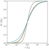 |
Fig. 3. Cumulative mass profiles of star clusters with equal masses and half-mass radii corresponding to the Dehnen models with(γ = 0, 1, 2 in red, green, and blue solid lines, respectively), and the Plummer model (black dashed line). |
Fujii et al. (2021b) showed (also see Li et al. 2019) that star clusters do not have a core during the gas embedded phase. This motivated us to consider the Dehnen models with γ > 0 (i.e., with a cuspy profile) in our study as well.
2.2. Recovering the residual gas
As mentioned earlier in this paper, we assume that in our model clusters star-formation happens with a constant SFE per free-fall time (ϵff = const) according to Parmentier & Pfalzner (2013). Thus following Shukirgaliyev et al. (2017), we can recover the density profile of the residual gas clump before gas expulsion, for a given stellar density profile, ρ⋆(r), SFE per free-fall time, ϵff, and star-formation duration, tSF. For the sake of clarity, we bring these expressions (Eqs. (A.1)–(A.7) Shukirgaliyev et al. 2017) here:
 (14)
(14)
 (15)
(15)
 (16)
(16)
 (17)
(17)
 (18)
(18)
 (19)
(19)
The solution from Shukirgaliyev et al. (2017) allows for the stellar density profile to be any centrally concentrated function. Since the gas density depends on the stellar density locally, the solution is also valid for clumpy structure of the stellar cluster.
To account for the residual gas potential in the case of Dehnen model clusters, we developed a new acceleration (read as external potential1) plug-in GPDehnen2 to the MHKHALO program (McMillan & Dehnen 2007) from the NEMO/falcON package (Teuben et al. 1995; Dehnen 2000, 2002), based on a previous GasPotential acceleration plug-in (Shukirgaliyev et al. 2017; Shukirgaliyev 2018). Together with GPDehnen acceleration plug-in, MKHALO program generates a single-mass N-body system, distributed in position-velocity space by the Dehnen model in virial equilibrium within the total gravitational potential of stars and gas. GPDehnen acceleration plug-in requires four parameters, namely, ϵff, tSF, γ, and aD to reproduce the gravitational potential of the residual gas. The stellar mass is set to the unity in N-body units. We also developed another method to generate our special initial conditions with AGAMA code (Vasiliev 2019). Both methods work very well and the generated N-body systems are in virial equilibrium within the external potential of the residual gas recovered by Eq. (14). We can re-assign the masses of the individual particles according to the chosen initial mass function (IMF), while keeping the total mass constant. This would introduce some perturbations locally, but it won’t change the total virial ratio of the generated N-body system. Therefore, it remains in virial equilibrium with the external potential after even after introducing the IMF.
In this study, similarly to previous studies, we adopt the SFE per free-fall time ϵff = 0.05. However, as it is clear from Eqs. (14)–(19), the density profile of the residual gas depends on the product of ϵff and tSF, rather than their individual values. Therefore, any values of ϵff and tSF can be assumed without changing the global SFE, while their product is preserved. From observations of star-forming regions, the SFE per free-fall time has been estimated to be about ϵff ≈ 0.01. The values of log ϵff varies from −2.5 to −1.3 depending on the method of measurement (see Fig. 10 in Krumholz et al. 2019). If we want the SFE per free-fall time to be ϵff = 0.01, the only changes to be applied to the adopted values of tSF, which becomes five times longer than in the case of ϵff = 0.05. It will not change anything else for the subsequent N-body simulations taking place after the instantaneous gas expulsion.
2.3. Measuring the SFE
Our model clusters exhibit centrally peaked SFE profiles due to the fact that stars have a steeper density profile than gas does, as a consequence of star formation taking place along a constant level of efficiency per free-fall time. That means (as noted earlier in this paper) SFE decreases as the radius increases. In the case of the Plummer model, the cumulative SFE converges to the total SFE at infinity because the residual gas mass converges as well (p ≈ 3.3). In the case of Dehnen models, the global SFE vanishes at an infinite radius. This is caused by the diverging mass of the residual gas, which has a power-law density profile with an index of (p ≈ 2.6 < 3). Therefore we need to define robustly the cluster outer radius to measure the value of SFE representing the global SFE of model clusters. Even in the case of the Plummer model, we had to determine the global SFE within some outer radius in order to maintain consistency with other studies. In the case of real star-forming regions, we cannot infinitely increase the outer radius, which would then start to account for neighboring star-formation regions, since molecular clouds usually contain several star-forming regions next to one another. There is no universal definition of the cluster outer radius for measuring the global SFE that can be found neither from theory or from the observations. This also sets some uncertainties upon comparisons of the models to the observations.
In previous studies (Shukirgaliyev et al. 2017), the Plummer model assumes clusters with an outer radius of Rout = 10aP = 7.66rh to measure the global SFE, which was then used to parameterize the set of models. However, neither Rout = 10aP nor Rout = 7.66rh have been found useful for the application of Dehnen models. Therefore, we faced a problem in choosing some universal outer edge with which to measure the global SFE in order to parameterize our Dehnen model clusters. If we applied the same logic as before and tried to catch at least 98 percent of stellar mass for the Dehnen models, the outer radius might go too much far out of the cluster space (e.g., > 38.5rh for γ = 0 or > 49rh for γ = 2 see Fig. 3). Therefore, we propose the following two options for measuring SFE when representing the cluster globally, as in the scope of this paper. In the first, following Shukirgaliyev et al. (2017), we use the global SFE redefined as
 (20)
(20)
where a⋆ is the scale radius of the chosen stellar density profile. For the Dehnen models, the mass fraction enclosed within 10a⋆ ≡ 10aD varies from 0.75 to 0.96 for different γ (see Fig. 4).
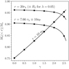 |
Fig. 4. Enclosed mass fraction of the Dehnen model clusters within different radii (RJ ≡ 20rh, 10aP ≡ 7.66rh, and 10aD) as a function of γ. |
Another option is to measure the SFE within the Jacobi radius of the stellar cluster, RJ, ignoring the residual gas mass. We understand that this definition of SFE as a Jacobi SFE cannot be universal, since the Jacobi radius of the same star cluster can vary depending on the adopted impact of the Galactic tidal field. Since we aim to compare our new results with the default (or so-called standard) models of Shukirgaliyev et al. (2017) (see also Shukirgaliyev et al. 2019), we adopt the impact of the tidal field of
 (21)
(21)
The adopted value of λ = 0.05 might seem to be too small compared to that of the observed open clusters varying around 0.1 and 0.2 in most cases (Piskunov et al. 2008; Portegies Zwart et al. 2010; Fujii & Portegies Zwart 2016). However, for the Solar neighborhood λ = 0.05 results in a mean density within half-mass radius, ρh ≈ 388ℳ⊙ pc−3, which is still in the range of the observed mean densities for clusters younger than 5 Myr (Lada & Lada 2003; Portegies Zwart et al. 2010; Fujii & Portegies Zwart 2016; Krumholz et al. 2019). According to Marks & Kroupa (2012), the observed open clusters were much denser (about 104ℳ⊙ pc−3) at their gas embedded phases. Also, the star formation simulations of Fujii & Portegies Zwart (2016), Fujii et al. (2021b,a) result in higher densities (> 102ℳ⊙ pc−3) for embedded clusters than for gas-free clusters after gas expulsion. Therefore, the adopted value of λ is consistent with the findings of other studies of embedded clusters. For the scope of this study, we considered model star clusters with the same stellar mass, M⋆, and the stellar half-mass radius, rh. Thus, the Jacobi SFE of our model clusters is:
 (22)
(22)
We chose the Jacobi SFE to parameterize our Dehnen models because it accounts for more than 95 percent of the stellar mass (for γ ≤ 2.1, Fig. 4), the local SFE drops down to about 0.6 percent (Fig. 5) at RJ, it does not depend on γ, and also it has a physical meaning for our model clusters. We plan to further discuss the robust measurements of the SFE and the outer truncation radius in a follow-up paper. In this study, we consider some of the simplest ways of measuring the SFE. Thus, in Fig. 5, we demonstrate the cumulative SFE (Eq. (6)) and local SFE (Eq. (5)) profiles of model clusters distributed by the Plummer model (black dashed lines) and the Dehnen models (γ = 0, 1, 2 in red, green, and blue solid lines) in thick and thin lines, respectively. Interestingly, Dehnen models with different γ result in a very similar cumulative SFE at r > rh if the radius is given in the units of rh. The local SFEs are similar even for about r > rh/2. Therefore, for Dehnen models with different inner slopes, measuring the global SFE within the radius r = xrh is preferable, then within r = yaD, where x and y are arbitrary numbers that are larger than the unity.
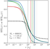 |
Fig. 5. Cumulative and local SFE profiles of model clusters with different stellar density profiles corresponding to the Dehnen model (γ = 0, 1, 2 in red, green, and blue solid lines) and the Plummer model (dashed lines), given in thick and thin lines, respectively. SFE per free-fall time of ϵff = 0.05 and the SF duration of tSF = 1 Myr (or equivalently ϵff = 0.01 and tSF = 5 Myr) were adopted to recover the density profiles of the residual gas for a cluster with M⋆ = 6000ℳ⊙ and rh = 1.23 pc. The vertical lines correspond to the stellar half-mass radius, rh (black solid line), 10aD (red, green, and blue solid lines corresponding to γ = 0, 1 and 2), 10aP (black dashed line), and the Jacobi radius, RJ (black dotted line), respectively. |
The SFE profiles in Fig. 5 have been calculated for model clusters with mass M⋆ = 6000ℳ⊙, half-mass radius rh = 1.23 for ϵff = 0.05 and tSF = 1 Myr (or equivalently for ϵff = 0.01 and tSF = 5 Myr). The chosen cluster half-mass radius corresponds to λ = 0.05 when a cluster moves on circular orbit on the Galactic disk plane at the Galactocentric distance of the Sun, Rorb = 8178 pc (Abuter 2019). We calculate the Jacobi radius of our stellar clusters according to Just et al. (2009, Eq. (13)):
 (23)
(23)
Here, β = 1.37 is the normalized epicyclic frequency, Ω = Vorb/Rorb is the angular speed of star cluster on a circular orbit (Just et al. 2009) at a distance of Rorb = 8178 pc with the circular speed of Vorb = 234.73 km s−1. We assume here that the total stellar mass resides inside the Jacobi radius, although a small fraction of stars might be outside, depending on the density profile.
Figure 6 demonstrates the SFE_J and SFE_10 as a function of tSF and ϵff. Figure 7 presents the relation between differently measured SFEs (SFE_J, SFE_10, eSFE, and LSF) for the Plummer and the Dehnen models. We note here that the SFE_J is the only measurement of SFE that depends on the environment. Other SFEs are independent of the impact of the tidal field of the host galaxy, but, instead, depend on the cluster density profile. Therefore, when we refer to the SFE_J, we mean the Jacobi SFE for λ = 0.05 in future, that is,SFE_J = SFEr(20rh).
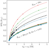 |
Fig. 6. So-called “global” SFEs as measured by SFE_J and SFE_10 of model clusters presented as functions of tSFϵff, represented by red, green, and blue solid lines for the Dehnen models with γ = 0, 1, and 2, and dashed lines for the Plummer model, in thick and thin lines, respectively. The marked points correspond to the parameterization values of SFE_J for the Dehnen models, and SFE10 for the Plummer models, respectively. |
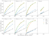 |
Fig. 7. Comparison of differently measured SFEs: SFE_J, SFE_10, eSFE, and LSF for the considered cluster models. The Jacobi SFE (SFEJ) has been chosen for parameterization of differently measured SFEs and is plotted in black as a one-to-one line. |
2.4. N-body simulations
We use the high-precision ϕ-GRAPE/GPU (Harfst et al. 2007; Berczik et al. 2013) direct N-body code with a fourth-order Hermite integrator, which uses GPU/CUDA based GRAPE emulation YEBISU library (Nitadori & Makino 2008) to perform our N-body simulations. The binary stars are not considered in this code; instead, the small-enough softening parameter ϵ = 10−4NB was introduced to avoid close encounters of stars. The evolution of single stars, including the mass-loss from the stellar wind are accounted through the updated SSE code (Hurley et al. 2000; Banerjee et al. 2020; Kamlah et al. 2021) integrated to ϕ-GRAPE/GPU code. In particular, we use the level C SSE code from Kamlah et al. (2021), which mainly differs from the original SSE code of Hurley et al. (2000) with regard to the stellar evolution prescriptions of massive stars. The new prescriptions include remnant-mass and fallback according to the rapid and delayed SNe models of Fryer et al. (2012), the pair-instability SNe (Belczynski et al. 2016) and Electron Capture SNe with small neutron star kicks (Belczynski et al. 2008). For more details, see Kamlah et al. (2021). In contrast to previous simulations (Shukirgaliyev et al. 2017, 2018, 2019), we take into account the natal-kick velocities of the SNe remnants in this study. Due to these differences in stellar evolutionary prescriptions, we decided to redo the simulations with the Plummer model clusters in the scope of this study. For the Galactic potential in our simulations, we use the three-component (bulge-disk-halo) axisymmetric Plummer-Kuzmin model (Miyamoto & Nagai 1975), which was previously used in Just et al. (2009) and our previous works (e.g., Shukirgaliyev et al. 2017, 2018, 2019), namely:
 (24)
(24)
where M, a, b are the mass, flattening parameter, and core radius of the component (see Table 1 in Shukirgaliyev et al. 2019). However, in this study we slightly tuned the halo mass to Mhalo = 7.2535 × 10¹¹ℳ⊙ to get the circular speed of Vorb = 234.73km s−1 at the Galactocentric distance of the Sun, Rorb = 8178 pc (Abuter 2019). Other parameters are kept as in Table 1 of Shukirgaliyev et al. (2019).
We adopted the following N-body units (NBU) and constants in our simulations of Dehnen clusters:
![Mathematical equation: $$ \begin{aligned} G=M_\star =r_\mathrm{h} =1\ [\mathrm{NBU} ]. \end{aligned} $$](/articles/aa/full_html/2021/10/aa41299-21/aa41299-21-eq27.gif) (25)
(25)
Model clusters (either with the Dehnen profiles or the Plummer profile) in the scope of this study have N⋆ = 10455 stars, leading to M⋆ = 6000ℳ⊙ when the stellar IMF (Kroupa 2001) with upper and lower stellar masses of mup = 100ℳ⊙ and mlow = 0.08ℳ⊙ is applied. The N-body units for the newly run Plummer model simulations are kept as in Shukirgaliyev et al. (2017).
2.5. Random realizations
We consider simulations of star cluster models for different SFE_J = [0.01, 0.03, 0.05, 0.07, 0.1, 0.15, 0.2, 0.3] and six different values of γ = 0, 0.5, 1, 1.5, 2, 2.5, for the Dehnen profiles and different SFE10 = [0.13, 0.15, 0.17, 0.2, 0.25] for the Plummer profile. We did not consider models with very low SFE_J = 0.01 for the Dehnen profiles with γ = 0 and γ = 0.5. For each model, we obtained nine random realizations, where we randomized the phase-space distribution of stars with three random seeds and the stellar IMF with three random seeds; that is, from MKHALO, we get three different models of single-mass N-body systems for a given set of parameters (model, i.e., Plummer or Dehnen with a given γ, and SFE_J defined by the product of ϵff and tSF ). Then for each model, we assigned stellar masses according to stellar IMF Kroupa (2001). In total, we performed 459 simulations (9 ⋅ (7 ⋅ 2 + 8 ⋅ 4)+5 ⋅ 9), including 414 simulations of Dehnen models and 45 simulations of Plummer models. When presenting our results, we demonstrate the mean and standard deviation of considered parameters (e.g., bound mass fraction) from the sample of nine random realizations of a given model.
3. Results
We looked at the evolution of bound mass fractions, Fb, of our star clusters within the first 150 Myr time-span as shown in Fig 8. As in our previous studies, we defined the bound-mass fraction as a ratio of the Jacobi mass at the current time, MJ, to the total initial stellar mass at the time of instantaneous gas expulsion, M⋆:
 (26)
(26)
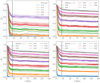 |
Fig. 8. Bound mass fraction evolution of clusters corresponding to the Plummer model (upper left panel) and the Dehnen (γ = 0, 1, 2 as indicated in legends) models during the first 150 Myr after instantaneous gas expulsion. The lines are color-coded by the corresponding SFEs as in the key. SFE10 has been used for the Plummer clusters, while SFE_J for the Dehnen clusters, respectively. The adopted end of violent relaxation tVR = 20 Myr is indicated by the vertical black line. |
The upper left panel of Fig. 8 corresponds to the new Plummer (with SNe natal kick and updated SSE) and the other panels to the Dehnen (γ = 0, 1, 2) model simulations, respectively. As we can see, there is a scatter from model randomization in both cases. Shukirgaliyev et al. (2018) showed that the most massive stars might cause sub-structure formation during the early expansion phase of cluster evolution after gas expulsion. In some cases these most massive stars can help clusters to survive with higher bound fraction than the average for a given SFE, as well as to leave the cluster with a low bound fraction by escaping early (see Fig. 1 in Shukirgaliyev et al. 2018). In Shukirgaliyev et al. (2019) we calculated the end of violent relaxation based on comparison of star cluster total mass-loss and the stellar evolutionary mass-loss. The assumed end of violent relaxation coincides with the moment when cluster total mass loss is almost equal to that of the stellar evolution. For the default models of Shukirgaliyev et al. (2019), with λ = 0.05 (i.e., also S0-models), the end of violent relaxation has been estimated to be tVR = 17.9 ± 2.3 Myr. In this study, for simplicity, we chose tVR = 20 Myr, as in Shukirgaliyev et al. (2017), which is consistent with estimation of Shukirgaliyev et al. (2019). From Fig. 8, it is clear that the difference of few Myr in the adopted time of the end of violent relaxation is still applicable. This tVR = 20 Myr is indicated by the vertical black line in of Fig. 8, to the right of which the bound mass fraction becomes almost constant. The shapes of the bound mass fraction evolution in both models are quite similar to those presented in previous studies (Shukirgaliyev et al. 2017, 2019). The wave-like shape corresponds to the vertical oscillation of the vertically escaped stars in the disk potential, bypassing the cluster Jacobi radius vertically. It is moderately small in case of the Dehnen models, where relatively compact bound cluster forms after gas expulsion, compared to the case of the Plummer model.
In case of low-SFE Dehnen model clusters, we can see that the violent relaxation seems to end earlier, as compared to the Plummer models. The Dehnen clusters have more compact and denser core than Plummer clusters. Also the Dehnen model clusters contain much greater amount of gas in the outer shells than the Plummer clusters. Thus, the unbound stars of low-SFE Dehnen clusters escape faster as they leave the compact core. More studies about the structural change of our model clusters will be discussed in upcoming papers. Nevertheless, tVR = 20 Myr seems to be quite a good estimation for the end of violent relaxation, when the final bound mass fraction, Fb20, is in focus.
In Fig. 9, we present the final bound mass fraction of our model clusters (i.e., at the end of violent relaxation tVR = 20 Myr) as a function of SFEs, measured in different ways. The survivability of model clusters are shown on the aspects of four different SFEs: on panel a of Fig 9 SFE is measured within 10aP for the Plummer models and 10aD for the Dehnen models, in the panel b we measure SFE within a Jacobi radius, < RJ ≡ 20rh for our simulations. In panels c and d we present results in the aspect of the LSF (i.e., SFE within a half-mass radius) and the eSFE (i.e., SFE based on virial ratio). The results for the Dehnen model clusters presented by red, green, and blue dots correspond to γ = 0, 1, 2, and for newly run Plummer models by blue plus symbols. The black crosses correspond to the default (or so-called “standard”) models of the previous Plummer model clusters (Shukirgaliyev et al. 2017, 2019). Additionally, in all panels, the results from Adams (2000) (dashed line) and Baumgardt & Kroupa (2007) (black star symbols, their instantaneous gas expulsion case) are presented as in the original papers, without any changes for reference. In the case of Baumgardt & Kroupa (2007) model, SFEs measured with different methods are equivalent to each other because the stars and gas have density profiles of the same shape. Therefore, it does not matter the radius within which SFE is measured since it will remain constant globally or locally in the scope of a given model. For their models, the eSFE is also equivalent to the total SFE (see Goodwin & Bastian 2006; Goodwin 2009). Therefore, their SFEs are quite consistent with those presented in Fig 9.
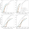 |
Fig. 9. SFE and bound mass fraction at the end of violent relaxation (t = tVR) for the Dehnen models (γ = 0, 1, 2 in red, green and blue points) and the Plummer model (orange crosses). The points correspond to the mean bound mass fraction of all random realizations of one model cluster, and error-bars correspond to the respective standard deviations. There are four different measurements of SFE considered in this plot. Panel a corresponds to SFE measured within ten scale radii corresponding to the models, namely, SFE10 = SFEr(10a⋆) as it was measured in Shukirgaliyev et al. (2017). Panel b presents SFE measured within the Jacobi radius, SFE_J = SFEr(RJ ≡ 20rh). Panels c and d present the survivability of model clusters as a functions of LSF and eSFE. The black crosses correspond to the default model of Shukirgaliyev et al. (2017, 2019), where the SNe remnant kick velocity is neglected. The results of Adams (2000) (dashes black line) and Baumgardt & Kroupa (2007) (black star symbols, the instantaneous expulsion case only) are plotted for the reference as given in the original publications. For the case of Baumgardt & Kroupa (2007), SFEs measured in all different ways are identical because the density profiles of gas and stars have the same shapes. |
We find that our Plummer model simulations result in a very similar final bound fraction, although the natal kick for SNe remnants has been included in the new simulations (compare orange crosses with the black dots in Fig. 9). This is explained by the late occurrence of SNe (three or more Myr after instantaneous gas expulsion), when the whole dynamics of the cluster is defined within the first few Myrs of expansion. Also, in the updated stellar evolution prescriptions, high-mass SNe remnant black holes have increased masses and no natal kick due to fallback mechanism (Belczynski et al. 2016; Kamlah et al. 2021), and, thus, they do not escape the cluster. Therefore, the difference in the remaining bound mass fraction between old and new simulations is not significant. Nevertheless, the minimum SFE needed for the Plummer model clusters to survive instantaneous gas expulsion stays within 0.15, if measured within 10aP, or lowered to 0.12 if measured within a Jacobi radius (only due to the measuring method of SFE). Corresponding values of differently measured SFEs are demonstrated in Fig. 7. In the case of LSF and eSFE, the survival SFE threshold are about 0.34 and 0.32, respectively, for the Plummer model clusters. Thus, they stay consistent with other simulations used Plummer model as initial condition for their star cluster simulations (Goodwin & Bastian 2006; Baumgardt & Kroupa 2007; Smith et al. 2011; Brinkmann et al. 2017; Lee & Goodwin 2016).
The Dehnen model clusters show much better survivability than the Plummer model clusters (see red, green, and blue dots in Fig. 9) in all aspects of SFEs, especially for low-SFE cases. The minimum SFE required to survive the instantaneous gas expulsion is 0.03 or 0.09 for the Dehnen γ = 0 model, depending on SFE measurement method, within < RJ or < 10aD, respectively. For the SFE_J = 0.03 ≡ SFE10 ≈ 0.05 model some random realizations of cluster models could not survive after violent relaxation. However, model clusters with a bit higher SFE (SFE_J = 0.05) confidently survive the instantaneous gas expulsion with bound mass fraction of above 0.10. The results from Dehnen models are quite similar when we look on the aspect of SFE_J, but very different when the global SFE is represented by SFE_10. This difference occurs only due to the method of the SFE measurement. As we noticed in Fig. 2, Dehnen models show very similar SFE values when the cumulative SFE is measured within the multiple of the half-mass radius. The Dehnen models demonstrate a good capability to survive the gas expulsion with low SFEs in the aspect of LSF and eSFE (see lower panels of Fig. 9). In this sense, the results obtained from the Dehnen models in the aspect of LSF also resemble the results obtained from hierarchically formed highly sub-structured cluster models of Farias et al. (2018) with live gaseous background or results of Li et al. (2019) obtained from their hydro-dynamical simulations of star cluster formation followed by N-body simulations. Although our models are calculated for the instantaneous gas expulsion, while the other two studies were done for more realistic (stellar feedback-driven) gradual gas expulsion cases.
In cases when SFEs are measured within ten model scale radii, the results on the survivability of the Dehnen (γ = 0) model and the Plummer model clusters are somewhat similar to each other in lower values; however, high-SFE clusters of the Dehnen models then show lower bound fractions than the Plummer model clusters.
Increasing the slope of the inner power law profile in Dehnen models also helps in demonstrating survival amid the consequences of the instantaneous gas expulsion with very low global SFE (i.e., SFE_J). Such an effect is already expected from their SFE profiles (see Fig. 5), i.e., the Dehnen models with higher γ have steeper SFE-profiles. Although, varying the inner power law slope does not make very big difference for higher-SFE model clusters (see Fig. 10).
 |
Fig. 10. Comparison of the bound mass fractions at the end of violent relaxation (t = tVR) of the Dehnen model clusters with different γ. Models with the same SFE_J are indicated with corresponding colors as in the key. |
In Fig. 10, we also present the differences between the final bound mass fractions of the Dehnen models across γ values. It shows a fine increase in the trends of the bound fraction with gamma for low-SFE clusters (SFE_J < 0.15). This indicates that having a cuspy profile at the moment of formation can help these low-SFE clusters to survive the consequences of gas expulsion quite well. The decreasing of the final bound fraction at higher γ for high-SFE clusters is due to the fact that their scale radii are larger than their half-mass radii. Thus, a significant fraction of star becomes unbound quickly after gas expulsion because of their large distance from the cluster center. For γ = 2.5, already 6 percent of the stellar mass becomes unbound immediately after gas expulsion, remaining beyond the new Jacobi radius (see Fig. 4).
We think that a better survivability of the Dehnen model clusters, compared to the Plummer model ones, comes from the relative shallowness of the density profiles of both the gas and stars. The latter results in more centrally peaked (steeper) SFE-profile in case of the Dehnen model clusters (see Fig. 5). Shukirgaliyev et al. (2019) already have shown that varying the cluster density allows the impact of the Galactic tidal field to avoid having a significant influence on the survivability of star clusters after gas expulsion. Therefore, we think that the steepness of the slope of SFE profile plays a significant role on the survivability of the stellar clusters after gas expulsion and subsequent violent relaxation, rather than the cluster’s central density.
4. Conclusions and discussion
In this study, we consider the survivability of star clusters with different density profiles after instantaneous gas expulsion. In particular, we consider model clusters corresponding to the Plummer model and the Dehnen model, with γ varying from 0 to 2.5 in virial equilibrium within the residual gas immediately before instantaneous gas expulsion. The density profiles of the residual star-forming gas corresponding to a given global SFE have been recovered based on the assumption that stars formed with a constant efficiency per free-fall time (Parmentier & Pfalzner 2013; Shukirgaliyev et al. 2017). Then we performed direct N-body simulations of clusters evolution after instantaneous gas expulsion, as if they are orbiting in the solar orbit, but exactly in the equatorial Galactic disk plane.
We re-simulated the Plummer model clusters with the updated stellar evolution prescriptions (Banerjee et al. 2020; Kamlah et al. 2021) and this time, the natal kick of SNe remnants was included. As we see from the results of our simulations, either accounting for or neglecting the natal kick velocity of SNe remnants does not really affect the survivability of star clusters after gas expulsion. This is because SNe happen three Myr after the instantaneous gas expulsion or later, since we assume that all stars in our model cluster enters the main sequence exactly at the time of gas expulsion. In real clusters, there is an age spread of less than five Myr (Reggiani et al. 2011; Kudryavtseva et al. 2012). However, only a few of the most massive (O-B) stars entering the main sequence can initiate the gas expulsion. The cluster dynamics after gas expulsion is already set by the gas potential. Then, the SNe takes place in the already expanding cluster or just after the violent relaxation, when the cluster is back to virial equilibrium with smaller amount of stars than it started out with originally. During the violent relaxation, only a fraction of massive stars undergo SNe. Also, in the updated stellar evolution prescriptions, high-mass black hole remnants have zero kick velocity and increased mass due to the fallback mechanism (Belczynski et al. 2008, 2016; Banerjee et al. 2020; Kamlah et al. 2021). Therefore, the SNe natal kick does not impact the final bound mass fraction, however, it can be significant with regard to the cluster structure and may affect the long-term evolution – two effects that are not considered in the scope of this study.
Here, we concentrate our focus on the question of whether the Dehnen model clusters survive the gas expulsion in the same way as in previously considered Plummer model clusters (Shukirgaliyev et al. 2017, 2019) or whether the process varies. Also, we discuss the problem of measuring the global SFE, both based on theory and the observations. The problem emerges when density profiles of stars and residual gas do not follow the same shape. In nearby star-forming regions Gutermuth et al. (2011) and, more recently, Pokhrel et al. (2020) found the power law correlation between surface densities of stars and gas to be  . That suggests that the stellar density profile has a steeper slope than that of the gas. Parmentier & Pfalzner (2013) explains such a behavior of gas and stars by their local density-driven clustered star formation model, where star-formation happens with a constant efficiency per free-fall time. As a consequence, in a given time-span, dense gas produces more stars than the diffuse gas. In such systems the local SFE is not equivalent to the global SFE, as it is in the models of Baumgardt & Kroupa (2007) and those used in studies referenced in their work. Also, the global SFE depends on the radius of sphere of measurement, thereby decreasing with increasing radius. Two different SFE measurements representing the global SFE are considered: one measured within stellar cluster Jacobi radius, RJ, ignoring the gas mass (SFE_J), and another measured as in Shukirgaliyev et al. (2017), less than ten times the model scale radii, SFE10 = SFEr(10a⋆). Also, we consider the local stellar fraction (LSF) – SFE measured within the stellar half-mass radius, rh, and the effective SFE (eSFE) – SFE defined based on the cluster virial state immediately after gas expulsion (see Eqs. (7)–(3) and the text in Sect. 1 for details). The Jacobi SFE is considered for the case when λ = rh/RJ = 0.05, thus SFE_J = SFEr(20rh). That is to say that the Jacobi SFE is the only method that is sensitive on the adopted environment (i.e., on λ). We also note that the Dehnen models with different inner slopes, γ, result in similar values of cumulative SFE if measured within the multiple of a half-mass radius (see Fig. 2).
In Sect. 3, we show the bound mass fraction of our model clusters, measured at the end of violent relaxation (t = 20 Myr) as functions of the considered SFEs (see Fig. 9). We found that the Dehnen model clusters have a better ability to survive gas expulsion with very low SFE than the Plummer model clusters. The minimum SFE needed to survive can be as low as SFE_J = 0.01 for the Dehnen model clusters with γ = 2 and 2.5. This is because the Dehnen model clusters have higher SFE in the inner part and lower SFE in the outer part when compared to the Plummer model. That is a consequence of having shallower density profiles for gas and stars in case of the Dehnen models than in the case of the Plummer models. Hence, the shallower the slope of stellar density profile, the lower the critical global SFE needed to survive the instantaneous gas expulsion. This statement applies to gas embedded stellar clusters formed in centrally concentrated and spherically symmetric gas clumps with a constant efficiency per free-fall time.
We conclude that the shallowness of the outer power law density profile of stellar cluster helps it to survive the instantaneous gas expulsion with low SFEs. In addition, star clusters with a cusp survive the consequences of instantaneous gas expulsion better than those without it. Additionally, the higher the slope of the cusp density power law profile, the higher the fraction of stellar mass remains bound to the cluster after violent relaxation.
In the NEMO/falcON package term acceleration plug-in is used for a plug-in accounting for additional acceleration from the background potential when generating the initial conditions of N-body system in virial equilibrium within some external gravitational potential.
Publicly available in the github portal:
Acknowledgments
We thank the referee for the helpful comments. This research has been funded by the Science Committee of the Ministry of Education and Science of the Republic of Kazakhstan (Grant No. AP08856149, AP08052197, and AP08856184). This work was supported by the Deutsche Forschungsgemeinschaft (DFG, German Research Foundation) – Project-ID 138713538 – SFB 881 (“The Milky Way System”) sub-project B2 – through the individual research grant ‘The dynamics of stellar-mass black holes in dense stellar systems and their role in gravitational-wave generation’ (BA 4281/6-1). This work was partly supported by the International Partnership Program of Chinese Academy of Sciences, Grant No. 114A11KYSB20170015 (GJHZ1810). BS, MS, TP, and MK are grateful for hospitality and support during visits to Silk Road Project of National Astronomical Observatories of Chinese Academy of Sciences. MS, MI, EP, PB, RS and AJ acknowledge the partial support by the Volkswagen Foundation under the Trilateral Partnerships grant No. 97778. PB and MI acknowledge the support by the National Academy of Sciences of Ukraine under the “Application of the high-performance parallel cluster computing in astrophysics and space geodesy”, No. 13.2021.MM. OB and EP acknowledge joint RFBR and DFG research project 20-52-12009 (N-body simulations). TP acknowledges the support by the European Research Council (ERC) under the European Union’s Horizon 2020 research and innovation program under grant agreement No 638435 (GalNUC). PB acknowledges support by the Chinese Academy of Sciences through the Silk Road Project at NAOC, the President’s International Fellowship (PIFI) for Visiting Scientists program of CAS, the National Science Foundation of China under grant No. 11673032. Facilities: Super-computing facilities at the Energetic Cosmos Laboratory of Nazarbayev University, Fesenkov Astrophysical Institute, Main Astronomical Observatory of the National Academy of Sciences of Ukraine, Zentrum für Astronomie der Universität Heidelberg, INASAN and Silkroad project at the National Astronomical Observatories of China/Chinese Academy of Sciences have been used for calculations in this study.
References
- Adams, F. C. 2000, ApJ, 542, 964 [NASA ADS] [CrossRef] [Google Scholar]
- Banerjee, S., Belczynski, K., Fryer, C. L., et al. 2020, A&A, 639, A41 [CrossRef] [EDP Sciences] [Google Scholar]
- Baumgardt, H., & Kroupa, P. 2007, MNRAS, 380, 1589 [NASA ADS] [CrossRef] [Google Scholar]
- Belczynski, K., Kalogera, V., Rasio, F. A., et al. 2008, ApJS, 174, 223 [NASA ADS] [CrossRef] [Google Scholar]
- Belczynski, K., Heger, A., Gladysz, W., et al. 2016, A&A, 594, A97 [NASA ADS] [CrossRef] [EDP Sciences] [Google Scholar]
- Berczik, P., Spurzem, R., Wang, L., Zhong, S., & Huang, S. 2013, in High Performance Computing, Third Int. Confer., 52 [Google Scholar]
- Brinkmann, N., Banerjee, S., Motwani, B., & Kroupa, P. 2017, A&A, 600, A49 [NASA ADS] [CrossRef] [EDP Sciences] [Google Scholar]
- Chen, Y., Li, H., & Vogelsberger, M. 2021, MNRAS, 502, 6157 [Google Scholar]
- Dehnen, W. 1993, MNRAS, 265, 250 [NASA ADS] [CrossRef] [Google Scholar]
- Dehnen, W. 2000, ApJ, 536, L39 [NASA ADS] [CrossRef] [PubMed] [Google Scholar]
- Dehnen, W. 2002, J. Comput. Phys., 179, 27 [NASA ADS] [CrossRef] [Google Scholar]
- Farias, J. P., Fellhauer, M., Smith, R., Domínguez, R., & Dabringhausen, J. 2018, MNRAS, 476, 5341 [NASA ADS] [CrossRef] [Google Scholar]
- Fryer, C. L., Belczynski, K., Wiktorowicz, G., et al. 2012, ApJ, 749, 91 [NASA ADS] [CrossRef] [Google Scholar]
- Fujii, M. S., & Portegies Zwart, S. 2016, ApJ, 817, 4 [NASA ADS] [CrossRef] [Google Scholar]
- Fujii, M. S., Saitoh, T. R., Hirai, Y., & Wang, L. 2021a, PASJ, 73, 1074 [NASA ADS] [CrossRef] [Google Scholar]
- Fujii, M. S., Saitoh, T. R., Wang, L., & Hirai, Y. 2021b, PASJ, 73, 1057 [NASA ADS] [CrossRef] [Google Scholar]
- Fukushima, H., & Yajima, H. 2021, MNRAS, 506, 5512 [NASA ADS] [CrossRef] [Google Scholar]
- Geyer, M. P., & Burkert, A. 2001, MNRAS, 323, 988 [NASA ADS] [CrossRef] [Google Scholar]
- Goodwin, S. P. 2009, Ap&SS, 324, 259 [NASA ADS] [CrossRef] [Google Scholar]
- Goodwin, S. P., & Bastian, N. 2006, MNRAS, 373, 752 [NASA ADS] [CrossRef] [Google Scholar]
- Goodwin, S. P., & Whitworth, A. P. 2004, A&A, 413, 929 [NASA ADS] [CrossRef] [EDP Sciences] [Google Scholar]
- Grasha, K., Calzetti, D., Adamo, A., et al. 2019, MNRAS, 483, 4707 [CrossRef] [Google Scholar]
- Gravity Collaboration, (Abuter, R., et al.) 2019, A&A, 625, L10 [NASA ADS] [CrossRef] [EDP Sciences] [Google Scholar]
- Grudić, M. Y., Guszejnov, D., Hopkins, P. F., Offner, S. S. R., & Faucher-Giguére, C.-A. 2021, MNRAS, 506, 2199 [Google Scholar]
- Gutermuth, R. A., Pipher, J. L., Megeath, S. T., et al. 2011, ApJ, 739, 84 [NASA ADS] [CrossRef] [Google Scholar]
- Harfst, S., Gualandris, A., Merritt, D., et al. 2007, New Astron., 12, 357 [NASA ADS] [CrossRef] [Google Scholar]
- Higuchi, A. E., Kurono, Y., Saito, M., & Kawabe, R. 2009, ApJ, 705, 468 [NASA ADS] [CrossRef] [Google Scholar]
- Hills, J. G. 1980, ApJ, 235, 986 [NASA ADS] [CrossRef] [Google Scholar]
- Hurley, J. R., Pols, O. R., & Tout, C. A. 2000, MNRAS, 315, 543 [NASA ADS] [CrossRef] [Google Scholar]
- Just, A., Berczik, P., Petrov, M. I., & Ernst, A. 2009, MNRAS, 392, 969 [NASA ADS] [CrossRef] [Google Scholar]
- Kainulainen, J., Federrath, C., & Henning, T. 2014, Science, 344, 183 [NASA ADS] [CrossRef] [Google Scholar]
- Kamlah, A. W. H., Leveque, A., Spurzem, R., et al. 2021, MNRAS, submitted [arXiv:2105.08067] [Google Scholar]
- Krause, M. G. H., Offner, S. S. R., Charbonnel, C., et al. 2020, Space Sci. Rev., 216, 64 [CrossRef] [Google Scholar]
- Kroupa, P. 2001, MNRAS, 322, 231 [NASA ADS] [CrossRef] [Google Scholar]
- Kruijssen, J. M. D., Schruba, A., Chevance, M., et al. 2019, Nature, 569, 519 [CrossRef] [Google Scholar]
- Krumholz, M. R., & Matzner, C. D. 2009, ApJ, 703, 1352 [NASA ADS] [CrossRef] [Google Scholar]
- Krumholz, M. R., McKee, C. F., & Bland-Hawthorn, J. 2019, ARA&A, 57, 227 [NASA ADS] [CrossRef] [Google Scholar]
- Kudryavtseva, N., Brandner, W., Gennaro, M., et al. 2012, ApJL, 750, 44 [Google Scholar]
- Lada, C. J., & Lada, E. A. 2003, ARA&A, 41, 57 [NASA ADS] [CrossRef] [Google Scholar]
- Lada, C. J., Margulis, M., & Dearborn, D. 1984, ApJ, 285, 141 [NASA ADS] [CrossRef] [Google Scholar]
- Lada, C. J., Lombardi, M., & Alves, J. F. 2010, ApJ, 724, 687 [NASA ADS] [CrossRef] [Google Scholar]
- Lee, P. L., & Goodwin, S. P. 2016, MNRAS, 460, 2997 [NASA ADS] [CrossRef] [Google Scholar]
- Leisawitz, D., Bash, F. N., & Thaddeus, P. 1989, ApJS, 70, 731 [NASA ADS] [CrossRef] [Google Scholar]
- Li, H., Vogelsberger, M., Marinacci, F., & Gnedin, O. Y. 2019, MNRAS, 487, 364 [NASA ADS] [CrossRef] [Google Scholar]
- Marks, M., & Kroupa, P. 2012, A&A, 543, A8 [NASA ADS] [CrossRef] [EDP Sciences] [Google Scholar]
- McMillan, P. J., & Dehnen, W. 2007, MNRAS, 378, 541 [NASA ADS] [CrossRef] [Google Scholar]
- Miyamoto, M., & Nagai, R. 1975, PASJ, 27, 533 [NASA ADS] [Google Scholar]
- Murray, N. 2011, ApJ, 729, 133 [NASA ADS] [CrossRef] [Google Scholar]
- Nitadori, K., & Makino, J. 2008, New Astron., 13, 498 [NASA ADS] [CrossRef] [Google Scholar]
- Parmentier, G., & Pasquali, A. 2020, ApJ, 903, 56 [CrossRef] [Google Scholar]
- Parmentier, G., & Pfalzner, S. 2013, A&A, 549, A132 [NASA ADS] [CrossRef] [EDP Sciences] [Google Scholar]
- Piskunov, A. E., Schilbach, E., Kharchenko, N. V., Röser, S., & Scholz, R. D. 2008, A&A, 477, 165 [NASA ADS] [CrossRef] [EDP Sciences] [Google Scholar]
- Plummer, H. C. 1911, MNRAS, 71, 460 [CrossRef] [Google Scholar]
- Pokhrel, R., Gutermuth, R. A., Betti, S. K., et al. 2020, ApJ, 896, 60 [NASA ADS] [CrossRef] [Google Scholar]
- Portegies Zwart, S. F., McMillan, S. L. W., & Gieles, M. 2010, ARA&A, 48, 431 [NASA ADS] [CrossRef] [Google Scholar]
- Rahner, D., Pellegrini, E. W., Glover, S. C. O., & Klessen, R. S. 2019, MNRAS, 483, 2547 [NASA ADS] [CrossRef] [EDP Sciences] [Google Scholar]
- Reggiani, M., Robberto, M., Da Rio, N., et al. 2011, A&A, 534, A83 [NASA ADS] [CrossRef] [EDP Sciences] [Google Scholar]
- Schneider, N., Bontemps, S., Girichidis, P., et al. 2015, MNRAS, 453, L41 [CrossRef] [Google Scholar]
- Shukirgaliyev, B. 2018, PhD thesis, Zentrum für Astronomie derUniversität Heidelberg, Astronomisches Rechen-Institut (Heidelberg: Mönchhofstr), D-69120, 12 [Google Scholar]
- Shukirgaliyev, B., Parmentier, G., Berczik, P., & Just, A. 2017, A&A, 605, A119 [NASA ADS] [CrossRef] [EDP Sciences] [Google Scholar]
- Shukirgaliyev, B., Parmentier, G., Berczik, P., & Just, A. 2019, MNRAS, 486, 1045 [CrossRef] [Google Scholar]
- Shukirgaliyev, B., Parmentier, G., Berczik, P., & Just, A. 2020, in Star Clusters: From the Milky Way to the Early Universe, eds. A. Bragaglia, M. Davies, A. Sills, & E. Vesperini, 351, 507 [NASA ADS] [Google Scholar]
- Shukirgaliyev, B., Parmentier, G., Just, A., & Berczik, P. 2018, ApJ, 863, 171 [NASA ADS] [CrossRef] [Google Scholar]
- Smith, R., Fellhauer, M., Goodwin, S., & Assmann, P. 2011, MNRAS, 414, 3036 [NASA ADS] [CrossRef] [Google Scholar]
- Teuben, P. 1995, in Astronomical Data Analysis Software and Systems IV, eds. R. A. Shaw, H. E. Payne, & J. J. E. Hayes, ASP Conf. Ser., 77, 398 [NASA ADS] [Google Scholar]
- Tutukov, A. V. 1978, A&A, 70, 57 [NASA ADS] [Google Scholar]
- Vasiliev, E. 2019, MNRAS, 482, 1525 [NASA ADS] [CrossRef] [Google Scholar]
- Verschueren, W. 1990, A&A, 234, 156 [Google Scholar]
- Verschueren, W., & David, M. 1989, A&A, 219, 105 [NASA ADS] [Google Scholar]
- Wall, J. E., McMillan, S. L. W., Mac Low, M.-M., Klessen, R. S., & Portegies Zwart, S. 2019, ApJ, 887, 62 [CrossRef] [Google Scholar]
- Wall, J. E., Mac Low, M.-M., McMillan, S. L. W., et al. 2020, ApJ, 904, 192 [Google Scholar]
All Figures
|
Fig. 1. Plummer-like power law density profiles of stellar clusters for q = 3, 4, 5, and of the corresponding initial gas, with p = 2, 2.6, 3.3. The density profiles of the initial gas were recovered according to the star cluster formation model of Parmentier & Pfalzner (2013), alike in Shukirgaliyev et al. (2017), for ϵff = 0.05, and tSF = 3 Myr. |
| In the text | |
|
Fig. 2. Volume density profiles of star clusters with equal masses and half-mass radii corresponding to the Dehnen models (γ = 0, 1, 2 in red, green and blue solid lines, respectively), and the Plummer model (black dashed line). The vertical lines show the corresponding scale radii, aD and aP with respective colors. |
| In the text | |
|
Fig. 3. Cumulative mass profiles of star clusters with equal masses and half-mass radii corresponding to the Dehnen models with(γ = 0, 1, 2 in red, green, and blue solid lines, respectively), and the Plummer model (black dashed line). |
| In the text | |
|
Fig. 4. Enclosed mass fraction of the Dehnen model clusters within different radii (RJ ≡ 20rh, 10aP ≡ 7.66rh, and 10aD) as a function of γ. |
| In the text | |
|
Fig. 5. Cumulative and local SFE profiles of model clusters with different stellar density profiles corresponding to the Dehnen model (γ = 0, 1, 2 in red, green, and blue solid lines) and the Plummer model (dashed lines), given in thick and thin lines, respectively. SFE per free-fall time of ϵff = 0.05 and the SF duration of tSF = 1 Myr (or equivalently ϵff = 0.01 and tSF = 5 Myr) were adopted to recover the density profiles of the residual gas for a cluster with M⋆ = 6000ℳ⊙ and rh = 1.23 pc. The vertical lines correspond to the stellar half-mass radius, rh (black solid line), 10aD (red, green, and blue solid lines corresponding to γ = 0, 1 and 2), 10aP (black dashed line), and the Jacobi radius, RJ (black dotted line), respectively. |
| In the text | |
|
Fig. 6. So-called “global” SFEs as measured by SFE_J and SFE_10 of model clusters presented as functions of tSFϵff, represented by red, green, and blue solid lines for the Dehnen models with γ = 0, 1, and 2, and dashed lines for the Plummer model, in thick and thin lines, respectively. The marked points correspond to the parameterization values of SFE_J for the Dehnen models, and SFE10 for the Plummer models, respectively. |
| In the text | |
|
Fig. 7. Comparison of differently measured SFEs: SFE_J, SFE_10, eSFE, and LSF for the considered cluster models. The Jacobi SFE (SFEJ) has been chosen for parameterization of differently measured SFEs and is plotted in black as a one-to-one line. |
| In the text | |
|
Fig. 8. Bound mass fraction evolution of clusters corresponding to the Plummer model (upper left panel) and the Dehnen (γ = 0, 1, 2 as indicated in legends) models during the first 150 Myr after instantaneous gas expulsion. The lines are color-coded by the corresponding SFEs as in the key. SFE10 has been used for the Plummer clusters, while SFE_J for the Dehnen clusters, respectively. The adopted end of violent relaxation tVR = 20 Myr is indicated by the vertical black line. |
| In the text | |
|
Fig. 9. SFE and bound mass fraction at the end of violent relaxation (t = tVR) for the Dehnen models (γ = 0, 1, 2 in red, green and blue points) and the Plummer model (orange crosses). The points correspond to the mean bound mass fraction of all random realizations of one model cluster, and error-bars correspond to the respective standard deviations. There are four different measurements of SFE considered in this plot. Panel a corresponds to SFE measured within ten scale radii corresponding to the models, namely, SFE10 = SFEr(10a⋆) as it was measured in Shukirgaliyev et al. (2017). Panel b presents SFE measured within the Jacobi radius, SFE_J = SFEr(RJ ≡ 20rh). Panels c and d present the survivability of model clusters as a functions of LSF and eSFE. The black crosses correspond to the default model of Shukirgaliyev et al. (2017, 2019), where the SNe remnant kick velocity is neglected. The results of Adams (2000) (dashes black line) and Baumgardt & Kroupa (2007) (black star symbols, the instantaneous expulsion case only) are plotted for the reference as given in the original publications. For the case of Baumgardt & Kroupa (2007), SFEs measured in all different ways are identical because the density profiles of gas and stars have the same shapes. |
| In the text | |
|
Fig. 10. Comparison of the bound mass fractions at the end of violent relaxation (t = tVR) of the Dehnen model clusters with different γ. Models with the same SFE_J are indicated with corresponding colors as in the key. |
| In the text | |
Current usage metrics show cumulative count of Article Views (full-text article views including HTML views, PDF and ePub downloads, according to the available data) and Abstracts Views on Vision4Press platform.
Data correspond to usage on the plateform after 2015. The current usage metrics is available 48-96 hours after online publication and is updated daily on week days.
Initial download of the metrics may take a while.