| Issue |
A&A
Volume 650, June 2021
|
|
|---|---|---|
| Article Number | A131 | |
| Number of page(s) | 9 | |
| Section | Stellar structure and evolution | |
| DOI | https://doi.org/10.1051/0004-6361/202140578 | |
| Published online | 18 June 2021 | |
A search for radio emission from double-neutron star merger GW190425 using Apertif⋆
1
Anton Pannekoek Institute, University of Amsterdam, Postbus 94249, 1090 GE Amsterdam, The Netherlands
e-mail: omboersma@gmail.com
2
ASTRON, the Netherlands Institute for Radio Astronomy, Oude Hoogeveensedijk 4, 7991 PD Dwingeloo, The Netherlands
3
Kapteyn Astronomical Institute, PO Box 800, 9700 AV Groningen, The Netherlands
4
Astronomisches Institut der Ruhr-Universität Bochum (AIRUB), Universitätsstrasse 150, 44780 Bochum, Germany
5
Astro Space Center of Lebedev Physical Institute, Profsoyuznaya Str. 84/32, 117997 Moscow, Russia
6
Dept. of Astronomy, Univ. of Cape Town, Private Bag X3, Rondebosch 7701, South Africa
7
Tricas Industrial Design & Engineering, Zwolle, The Netherlands
8
Cahill Center for Astronomy, California Institute of Technology, Pasadena, CA, USA
9
Dept. of Electrical Engineering, Chalmers University of Technology, Gothenburg, Sweden
10
Department of Physics, Virginia Polytechnic Institute and State University, 50 West Campus Drive, Blacksburg, VA 24061, USA
11
CSIRO Astronomy and Space Science, Australia Telescope National Facility, PO Box 76, Epping, NSW 1710, Australia
12
Sydney Institute for Astronomy, School of Physics, University of Sydney, Sydney, NSW 2006, Australia
13
Rijksuniversiteit Groningen Center for Information Technology, PO Box 11044, 9700 CA Groningen, The Netherlands
Received:
16
February
2021
Accepted:
7
April
2021
Context. Detection of the electromagnetic emission from coalescing binary neutron stars (BNS) is important for understanding the merger and afterglow.
Aims. We present a search for a radio counterpart to the gravitational-wave (GW) source GW190425, a BNS merger, using Apertif on the Westerbork Synthesis Radio Telescope (WSRT).
Methods. We observed a field of high probability in the associated localisation region for three epochs at ΔT = 68, 90, 109 d post merger. We identified all sources that exhibit flux variations consistent with the expected afterglow emission of GW190425. We also looked for possible transients. These are sources that are only present in one epoch. In addition, we quantified our ability to search for radio afterglows in the fourth and future observing runs of the GW detector network using Monte Carlo simulations.
Results. We found 25 afterglow candidates based on their variability. None of these could be associated with a possible host galaxy at the luminosity distance of GW190425. We also found 55 transient afterglow candidates that were only detected in one epoch. All of these candidates turned out to be image artefacts. In the fourth observing run, we predict that up to three afterglows will be detectable by Apertif.
Conclusions. While we did not find a source related to the afterglow emission of GW190425, the search validates our methods for future searches of radio afterglows.
Key words: gravitational waves / stars: neutron / radio continuum: stars
Data used to plot the images in this work has been uploaded at: http://doi.org/10.5281/zenodo.4672444
© ESO 2021
1. Introduction
The Advanced LIGO detector network started its first observing run in 2015 and was joined by the Advanced Virgo detector for the second run (Aasi et al. 2015; Acernese et al. 2014). These runs yielded ten detections of binary black hole (BBH) mergers and one binary neutron star (BNS) merger (LIGO Scientific Collaboration & Virgo Collaboration 2019). The successful detection of electromagnetic (EM) emission associated with the sole BNS merger, GW170817 (LIGO Scientific Collaboration & Virgo Collaboration 2017), included the dynamical ejecta of a kilonova (KN; see e.g., Chornock et al. 2017; Coulter et al. 2017), the short gamma-ray burst (SGRB) GRB170817A (e.g., Abbott et al. 2017), and the afterglow of the jet interacting with the interstellar environment (e.g., Alexander et al. 2017; Haggard et al. 2017; Hallinan et al. 2017). Together these studies brought forth an exciting new chapter in multi-messenger astronomy. In the first half of the third observing run (O3), the Advanced LIGO and Virgo detector network detected 39 candidate compact binary coalescences (Abbott et al. 2020c). The first detection of a BNS candidate in this run, LIGO/Virgo S190425z, later confirmed as GW190425 (Abbott et al. 2020a), occurred on April 25, 2019. It was observed solely by the Advanced LIGO Livingston detector at a distance of  Mpc. The Advanced Virgo detector was also operational but did not detect the merger. The localisation capabilities of just a single detector are poor and, as such, the LAL Inference (Veitch et al. 2015) sky map (LALInference.fits.gz) for this source, shown partly in Fig. 1, has a 90% credible localisation region on the sky of 7461 deg2. Nonetheless, follow-up campaigns using optical and/or infrared facilities were performed directly after the merger. Campaigns such as GROWTH (Coughlin et al. 2019) and GRANDMA (Gendre et al. 2019) aimed to find coincident EM emission from a KN or SGRB counterpart. While these efforts covered a large region of the probability map, the searches did not lead to identifying a viable source of the gravitational-wave (GW) emission.
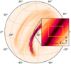 |
Fig. 1. Part of the LIGO/Virgo localisation sky map on the northern hemisphere for GW190425. The full sky map has a 90% credible sky area of 7461 deg2, which reduces to 1378 deg2 at the 50% level. The blue contour encompasses the 50% credible sky area on this part of the sky. The inset shows the approximate Apertif FOV in yellow. |
In the absence of an optical or infrared counterpart, radio emission may provide the only way to localise the source at later times (Hotokezaka et al. 2016). In order to maximise the probability of detecting coincident radio emission, a relatively large field of view (FOV) and high sensitivity are necessary. In this work, we present a follow-up of GW190425 with the new Apertif phased array feeds (PAFs; Oosterloo et al. 2010; Adams & van Leeuwen 2019) on the Westerbork Synthesis Radio Telescope (WSRT). While the FOVs of these PAFs, at 9.5 deg2 (van Leeuwen et al., in prep.), are one of the largest in the world, they are still dwarfed by the error region. As the detection of an afterglow has the potential to significantly further our understanding of such mergers, we performed the search against these odds. In Sect. 2 we discuss our observations and the data reduction methods. We examine the flux consistency between our three observations in Sect. 3. In Sect. 4 we describe the search for radio transients in our observations. We make predictions for the amount of radio afterglows Apertif will detect in the fourth and future GW detector network observing runs in Sect. 5, and we conclude in Sect. 6.
2. Observations and data reduction
We observed a target field with Apertif, which was chosen to cover a 9.5 deg2 region of high probability in the localisation sky map. This field centred on coordinates α = 16h25m12s, δ = +17° 47′24″ (J2000) was observed three times for 12 h at ΔT = 68, 90, 109 d post merger. We refer to these observations as epoch 1, 2, and 3, respectively. Table 1 gives a summary of the observations. For epoch 2, all 12 Westerbork antennas with Apertif PAFs (on the fixed, equidistant Radio Telescopes RT2..RT9 plus the movable dishes RTA..RTD) were operational. For epoch 1 antenna RTD was not operational and for epoch 3 antenna RT2 was not in use. Furthermore, data from antenna RTC were not included in the processing of epoch 1 because this dish suffered from delay issues.
Overview of the three epochs of observations with Apertif.
The field is covered by 40 partially overlapping beams formed from the PAFs with a full width at half maximum (FWHM) of ∼35 arcminutes each on the sky. The data have a centre frequency of 1280 MHz with 300 MHz of bandwidth being recorded. The flux and bandpass calibrator 3C 147 was either observed before (first and third epochs) or after (second epoch) the observation for 3 min for each of the 40 Apertif beams. The data were imaged for each beam separately using Apercal, the Apertif imaging pipeline (Adebahr et al., in prep.), version 2.5. Owing to high levels of radio frequency interference (RFI) in the lower part of the band, only the upper 150 MHz is processed. As the signal is expected to be broad band, the frequency coverage itself is not overly important, but reducing the bandwidth by a factor of 2 results in an increase in the image noise, and thus the detection threshold, by a factor of  (Adams et al., in prep.)
As part of the pipeline, automatic flagging of RFI is performed using AOFlagger (Offringa et al. 2010, 2012). This resulted in ∼14%, 21%, and 12% of the processed data per beam being flagged, on average, owing to RFI for epochs 1, 2, and 3, respectively. Additionally, the first 12 min of observation for epoch 2 were flagged manually because the dishes were not properly settled on source. Including these data resulted in artefacts in the continuum image, while flagging the data only had a minor impact on the overall sensitivity.
For epochs 1 and 3, all reduction steps including cross-calibration, direction-independent self-calibration, imaging, and cleaning were done using standard pipeline parameters (Adebahr et al., in prep.). In particular, the intervals of the self-calibration solutions, used to update the solutions obtained from the calibrator observations, were derived automatically. For epoch 2, however, solution intervals of 30 s, shorter than derived by the pipeline, were necessary to suppress notable phase artefacts in the cleaned continuum images.
The final data product per beam produced by Apercal is a multi-frequency Stokes I image created over the full processed frequency range. A mosaicking script then combines the beam continuum images using a linear algorithm. An inverse-squared weighting, based on preliminary primary beam response models of Apertif, is used to adjust for decreasing sensitivity away from the phase centre. Additionally, different parts of the observation were flagged per beam, affecting the resolution. To ensure a consistent resolution across the mosaic, the images are convolved to the common highest possible resolution before making the mosaic. For epochs 1 and 3, one beam failed internal data quality checks implemented in the pipeline and was not used when creating the mosaics. For epoch 2, nine beams failed internal data quality checks and were not used in the mosaic. As a consequence, epoch 2 has a slightly reduced FOV compared to the other epochs. We show the mosaic of the third epoch in Fig. 2.
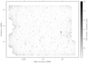 |
Fig. 2. Apertif mosaic, centred on 16:25:12.0, 17:47:24.0, covering a region of high probability in the localisation skymap of GW190425. The mosaic, our third epoch, was observed 109 days post merger. |
The beam size of epoch 2 is 50 arcsec × 12 arcsec and has a major axis position angle PA = −0.1°, which is consistent with that at epoch 3 of 48 arcsec × 11 arcsec (PA = −0.6°). The beam size of epoch 1, that is 90 arcsec × 23 arcsec (PA = 0.6°), is considerably worse. For epoch 1, we lacked the longest baselines, as data from antennas RTC and RTD could not be used. The best rms noise sensitivity reached is ∼70 μJy, 60 μJy and 50 μJy, for epochs 1, 2, and 3, respectively. This sensitivity decreases closer to the edges of the mosaics or around bright sources as a consquence of direction-dependent errors. We inspect the stability of the source fluxes in the next section.
3. Flux consistency between epochs
The radio sky is relatively quiet compared to other wavelengths; it has an estimated transient rate of less than 0.37 deg−2 at 1.4 GHz for sources with a peak flux density greater than 0.21 mJy (Mooley et al. 2013). Furthermore, most sources should not exhibit any variation in their flux besides measurement errors due to noise (see e.g., Sarbadhicary et al. 2020 and references therein). Because the observations were taken during the Apertif commissioning phase, it is important to test how stable the measured source fluxes are between the epochs. To this extent, the mosaics of each epoch were analysed using the source finder PyBDSF (which is also used in the Apercal pipeline; Mohan & Rafferty 2015) and the integrated fluxes for unresolved sources with a positional match within 10 arcsec were compared. We used the local noise map computed by PyBDSF and selected sources 5σ above the local rms noise level. Surrounding pixels above the 3σ level were also used for source fitting. We constrained the shape of the Gaussian fit to the restoring beam.
The flux scale is consistent between all epochs, which is within the usual range of flux uncertainties for imaging observations. We recover a median of the ratio in fluxes of 1.00, 0.97, and 0.96 between epochs 1 and 2, epochs 1 and 3, and epochs 2 and 3, respectively. To quantify the scatter in the fluxes, for each source we define
where Δfx, y is the absolute value of the relative difference in integrated flux and fint, x and fint, y are the integrated fluxes in epochs x and y.
The scatter in the radio fluxes is higher than expected; the median values of Δf1, 2, Δf1, 3, and Δf2, 3 are 13.7%, 10.6%, and 8.9%, respectively. We plot these statistics as a function of integrated flux in Fig. 3 for each combination of epochs. The scatter does not exhibit a strong flux dependence beyond what could be expected in terms of rms noise errors. We suspect that the quality of the phase calibration is the main source of this scatter. We discuss these errors, other possible causes, and the implications in our search for the afterglow in the next section.
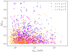 |
Fig. 3. Integrated flux vs. absolute value of relative difference in flux Δfx, y, defined in Eq. (1). This is calculated for epochs 1 and 2 (blue circles), epochs 1 and 3 (pink diamonds), and epochs 2 and 3 (orange crosses). The scatter is larger than what could be expected in terms of rms noise error with median values of Δf1, 2, Δf1, 3, and Δf2, 3 of 13.7%, 10.6%, and 8.9%, respectively. |
4. Search for the afterglow of GW190425
4.1. Radio variables and transients search
We made use of the LOFAR Transients Pipeline (TraP; Swinbank et al. 2015) to detect variable sources or transients in our observations. The TraP identifies sources over multiple epochs and constructs light curves for each source. From these light curves, statistics are calculated that can be used to quantify the variability of sources. For sources that are only identified in one epoch, a light curve cannot be constructed. Instead, using TraP we assigned a candidate transient classification to these sources based on their signal-to-noise-ratio (S/N) properties. A detailed explanation of TraP and the associated variability statistics is provided in Swinbank et al. 2015.
We set up TraP such that pixels with a flux count 5σ above the local rms noise level are identified as a source and surrounding pixels with a flux count 3σ above the noise become a part of that same source. The Gaussian fit that is then performed on the source to measure its flux density is constrained to have the same shape as the restoring beam. The dimensionless de Ruiter radius (de Ruiter et al. 1977), which is used to associate sources between epochs based on their angular separation, is set to the default value of 5.68. Furthermore, matching sources between epochs should have an angular separation of less than one semi-major axis of the restoring beam.
For sources with flux density measurements in two or three epochs, the reduced chi-squared statistic η and the fractional variability statistic V are calculated by TraP from the resulting light curve. A Gaussian function is fit to the distribution of both statistics in logarithmic space with mean and standard deviation μV, σV and μη, ση, respectively. Sources with both η and V significantly higher than the mean values of their distributions are identified as candidate variable sources. Thresholds for both metrics to separate such variables from stable sources can be chosen somewhat freely. Different thresholds influence recall and precision rates of the produced set of candidate variables considerably (Rowlinson et al. 2019). We followed Dobie et al. (2019) and specified a source as candidate variable if both η > μη + 1.5ση and V > μV + 1σV.
4.2. Expected afterglow emission of GW190425
To search for the radio afterglow of GW190425, we aim to select the potential candidates identified by TraP that have a flux evolution consistent with the expected afterglow emission. We based the criteria for emission partly on the light curve of the sole radio counterpart detected to date: that of GW170817. That event peaked at  (Mooley et al. 2018a), which is significantly later than our last epoch at ΔT = 109 d post merger. In population studies (Duque et al. 2019), however, a significant fraction of BNS-merger afterglows peak closer to our first or second epoch. Given this range, peak time is not a criterion for candidate selection per se. Even so, these jet-dominated afterglows should display only a single rise and decline in flux (Hotokezaka et al. 2016; Dobie et al. 2019), as observed in GW170817 (Mooley et al. 2018a,b; Ghirlanda et al. 2019). We therefore excluded sources with a decrease in flux density from epochs 1 to 2 and an increase in flux density from epochs 2 to 3.
If the afterglow emission of GW190425 exhibits the same flux evolution as GW170817, the associated radio source should be selected by TraP as an outlier in flux variability compared to the general population of radio sources. The scatter in fluxes mentioned in Sect. 3, however, might hinder our ability to detect the afterglow emission. We can estimate the expected increase in flux density using the light curve of GW170817 (Mooley et al. 2018a). The radio flux would have increased by ∼26% between the time of our epochs 1 and 2 and by ∼17% between the time of our epochs 2 and 3. These increases are still larger than the median scatter in our observations. Some models predict even stronger changes in flux over the timescale of our observations (Hotokezaka et al. 2016). Thus, we feel confident that a radio source of the afterglow of GW190425 should still be picked up as an outlier in variability. Even so, the significance of such a detection is low. We show the results of our search next.
4.3. Candidate variables
We obtained the following fit to the distributions of V and η in logarithmic space: μV = −0.97, σV = 0.38 and μη = 0.16, ση = 1.07. This corresponds to thresholds of η > 59 and V > 0.25. Using these thresholds, we recovered 30 candidate variables in our observations. From the 30 candidate variables, we selected those sources with flux measurements consistent with the expected afterglow emission. This resulted in 25 candidate variables possibly associated with GW190425 in our observations. After further manual inspection, 20 candidates in regions of increased noise, for example close to the edges of the mosaics, were found to have unreliable flux measurements and were discarded.
The 5 remaining candidates were cross matched with the GLADE catalogue (Dálya et al. 2018) within a 30 arcsec radius (corresponding to ≲20 kpc offset) to look for possible host galaxies. No galaxies were found within 3σ of the estimated luminosity distance  Mpc (90% credible intervals) of GW190425 (Abbott et al. 2020a). We conclude that none of these 5 candidates are a source of the afterglow emission of GW190425. Possible other origins of their variability are discussed in Sect. 4.5. For completeness, we list their properties in Table 2.
Overview of the five candidate variables found in our observations with flux measurements consistent with the expected afterglow emission of GW190425.
4.4. Candidate transients
Sources with only one flux density measurement can appear in any of the three epochs to be consistent with the expected afterglow emission. The TraP found 291 such sources in our observations, all in the third epoch. Upon manual inspection, most of these sources seem to be present in previous epochs. We suspect that they were not identified as a source because their shape does not match the restoring beam. We checked this hypothesis by running TraP without the previously mentioned restoring beam constraint. This led to substantially more sources being properly recognised in the first two epochs and not identified as a new source in the third epoch. However, many more image artefacts were now incorrectly being identified as a new source instead. We thus opted to continue with the restoring beam constraint in place.
To filter out most sources that were either in an area with high noise or whose shape was inconsistent with the restoring beam in previous epochs, we made use of their S/N calculated by TraP in the best noise region of the epoch with the previous lowest rms value (Swinbank et al. 2015). If the S/N in the best noise region crossed our detection threshold plus some extra margin M, the source was determined to be a candidate transient. The margin M that is chosen depends on the quality of the observations and desired recall and precision rates of the set of possible transients (see Rowlinson et al. 2019 for an in depth discussion). Setting M = 34 (Rowlinson et al. 2019) worked well to cut out most easily identifiable false positives in our candidate transient set. This narrowed down our search to 55 transient candidates. After manual inspection, all candidates were determined to result from either direction-dependent errors around bright sources or noise artefacts at the edges of the mosaics. Thus, we identified no transients in our observations as a source of the afterglow emission of GW190425.
4.5. Discussion
The ideal observing campaign for detecting a radio counterpart to GW190425 in our FOV involves a considerable number of repeat visits and an image quality approaching the theoretical sensitivity limit. The study we present has not yet met these specifications. Below we describe the factors that limited our ability to detect the afterglow.
For sources with flux density measurements in only a few epochs, the reduced chi-squared statistic η can vary appreciably over these epochs (Rowlinson et al. 2019). In general, the three epochs we observed might not be enough for most sources to robustly determine this measure for the stability of their light curve. Furthermore, this stability is also impacted by the general systematic variability mentioned in Sect. 3. Outliers in variability are less apparent when the scatter in flux between observations is already substantial for most sources. Thus, the distribution of η in log space becomes wider, which is apparent in the large value of the standard deviation ση from the Gaussian fit to η. For reference, Fig. A.1 shows a histogram of the two-dimensional distribution of η and V with the large spread in η clearly visible.
We presume the source of the general systematic variability in our observations to be related to the data reduction. We deem the main source of error to be the quality of the phase calibration. If the phases are not sufficiently calibrated, the emission from point sources is partially spread out rather than point-like. This can affect the flux that is measured in the source-finding procedures. Besides the resulting scatter in fluxes between the epochs, these calibration errors were also apparent when using TraP to find transients. Many sources were not properly recognised across the epochs owing to their inconsistent shape. This produced many false positives in our candidate transient set.
Uncertainties in the observations for the primary beam models could also increase the scatter in the flux measurements. Two possible complications are, for example, strong RFI during these observations and the malfunctioning of individual elements. Strong RFI could interfere with the measurements of the primary beam response. The frequency range used in our primary beam model, however, is normally relatively RFI free. We thus do not expect this to be a big influence. Some antennas might have a deformed primary beam shape because of malfunctioning individual elements. This may not be taken into account in the global primary beam model used, which is averaged across all antennas. The above and other factors can change on timescales shorter than the time between our epochs.
The influence of such variations in the mosaics would be partially compensated at low levels of the primary beam response. In this case, the beams overlap which suppresses model errors. Strong changes in the inner part of the beam would not be compensated as much. For epochs 1 and 2, the same set of primary beam models, closest in observation time to these epochs, were used. Epoch 3 was corrected with a different set of models. To measure any fluctuations between the two sets of models, we made a mosaic of the primary beam weights for each set. Between the two mosaics, the difference is at most ∼4% at the centre of the beams; variations are often below 1% at the edges. These fluctuations are thus too small to be the main source of the systematic variability in flux.
Sources that are near very bright sources are additionally affected by their direction-dependent errors. These errors gave rise to a non-Gaussian distribution of the noise in parts of our images which impeded accurate flux measurements. We suspect that for four of the five candidates in Sect. 4.3 their variability is due to these errors. They are relatively close to the same bright source and their relative change in flux between each epoch is similar (see row 2–5 in Table 2). The other candidate, first row in Table 2, also has a similar light curve evolution but is not particularly close to the other candidates. The shape of this source deviates from the restoring beam in epoch 1, likely as a result of the insufficient phase calibration, and presumably does not have its flux accurately measured in this epoch. As the flux is constant within the errors between epochs 2 and 3, we believe that the variability of this source, evident in the large values for η and the fractional variability V, is a result of the calibration error in epoch 1. The characteristic rings resulting from the direction-dependent errors also triggered a lot of false positives in the candidate transients set. Reducing these errors is an active area of development for Apercal. In Sect. 5.1, we detail a manual reprocessing of a few Apertif beams to improve the image quality.
In summary, a number of aspects of our search can be improved for future follow-up campaigns. Their impact would foremost be to reduce the number of false-positive candidates. Any sufficiently bright transients in our observing field would still have been detected.
5. Future observing prospects
5.1. Improvements in Apertif Imaging
The success of future afterglow searches with Apertif is partly contingent on the achievable image quality. The first Apertif survey data release (Adams et al., in prep.) has shown that noise levels down to 30 μJy and good image quality are regularly attained using automatic Apercal pipeline processing. While the automatic processing did not reach a similar quality for our observations, future reprocessing of the data could potentially yield improvements with updated versions of Apercal1.
To investigate this prospect, we reprocessed a few centre Apertif beams as a demonstration, using WSClean (Offringa et al. 2014) and DPPP (van Diepen et al. 2018). First, a further cross-calibration was applied to the data using a mask derived from the NVSS survey (Condon et al. 1998). This was followed by two cycles of direction-independent calibration and imaging in a standard way on minute solution intervals. Then the sources with strong artefacts were identified in the images and the corresponding directions were stored. Finally, additional direction-dependent calibration was performed in these directions to solve for both amplitude and phase variations on an hour solution interval.
We show a cut-out of the continuum image for beam “00” of epoch 2 in Fig. 4. The image on the left was made with Apercal, while the image on the right was manually reprocessed as described. Compared to Apercal, the side lobes of the bright source in the centre are better suppressed in the reprocessed image. Furthermore, the rings from the direction-dependent errors around this source are nearly gone. Noise levels are improved reaching ∼45–50 μJy in the centre of the reprocessed image. For epoch 3, the manual reprocessing of beam “00” gives similar improvements, while for epoch 1 the difference with Apercal is less pronounced.
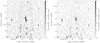 |
Fig. 4. Continuum image for beam “00” of epoch 2 made with Apercal (left) and manually reprocessed (right, see text for details). Image quality is improved in the reprocessed image with better side lobe suppression of the central bright source and less visible rings from direction-dependent errors. |
For bright sources with integrated fluxes above a few millijansky, the fluxes were consistent within 5% in the reprocessed images of epochs 2 and 3 for beam ‘00’. Compared to the ∼10% scatter in the Apercal images for such sources, this is a noticeable improvement that points to the source shapes being more consistent between the two epochs. It is difficult, however, to measure the overall scatter in flux based on a single beam as the number of faint sources is limited. To measure if the scatter decreased for faint sources too, we did an initial comparison in flux between mosaics of seven reprocessed centre beams for epochs 2 and 3. No major changes in the scatter were present in the integrated flux between the epochs compared to the results of Sect. 3. Of the few reprocessed beams, beam ‘00’ had the most obvious improvements in image quality. We thus did not find a universal improvement in image quality across beams. We reason that improvements are unlikely when running the reprocessed data through TraP to search for variable sources. Still, the direction-dependent calibration does reduce artefacts. This will lead to fewer false positive transients in our future afterglow searches.
We conclude that more observational epochs, further characterisation and understanding of the Apertif system, and improvements in the pipeline will greatly benefit our search for radio counterparts to BNS mergers. In the next section, we describe the prospects for finding these counterparts in the fourth and future observing runs of the GW detector network.
5.2. Expanding GW network of detectors
The fourth observing run (O4) of the GW detector network is expected to commence in 2022, although the early suspension of O3 has made the start date and the anticipated detector sensitivities more uncertain. In this section, we use the numbers for sensitivities outlined by the KAGRA Collaboration, LIGO Scientific Collaboration and Virgo Collaboration (Abbott et al. 2020b). Four detectors are planned to be operational for one year in O4: the two Advanced LIGO (aLIGO) detectors at design sensitivity; the Advanced Virgo (AdV) detector in its Phase 1 upgrade; and the newest addition, KAGRA (Somiya 2012; The KAGRA Collaboration 2013). During this year, the aLIGO detectors, AdV, and KAGRA will have anticipated BNS ranges R of 160–190 Mpc, 90–120 Mpc, and 25–130 Mpc, respectively. Importantly, from the  BNS events that are expected in total, 38–44% of these events are predicted to have a 90% credible region on the sky smaller than 20 deg2. This can be covered with just three Apertif pointings. While the localisation region on sky will likely be drastically reduced, the increase in BNS range will mean that more events will be detected at larger luminosity distances in O4. This will decrease our ability to detect the radio afterglow resulting from the inverse square relation between the radio flux and luminosity distance.
As a point of reference, we show a fit to the radio light curve of the afterglow of GW170817 (Mooley et al. 2018a) in Fig. 5 in blue with the best achieved 3σ Apertif sensitivity indicated in black. We would have been able to detect the emission if Apertif was operational at the time but this would not have been possible if the merger happened much further out. Just one observation would still yield a rather marginal detection. It is thus essential to regularly sample the light curve across multiple epochs to obtain a robust detection with physical information. In particular, the peak and the subsequent decay of the light curve should be monitored carefully. Certainly, the decay rate gives crucial information about the physical processes of the BNS merger (see Mooley et al. 2018a and references therein). If we had observed GW170817 on the same days post merger as our observations for GW190425 (orange stripes) in Fig. 5, we would have detected the afterglow in the last two observations.
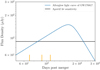 |
Fig. 5. Fit to radio light curve of afterglow of GW170817 (Mooley et al. 2018a) in blue. The curve is plotted on a log-log scale to easily show the power-law dependence. The 3σ Apertif design sensitivity is shown in black. Three observations on the same days post merger as our observations for GW190425 are shown as orange stripes. |
To quantify our ability to detect radio counterparts to BNS events in O4 and beyond, we follow the population study in Duque et al. (2019) and include Apertif. We summarise the criterion for radio detection and GW detection of the merger in the next section. We refer to their work for a detailed explanation of the afterglow model and the distribution of BNS population parameters.
5.3. Forecasts for radio detections of binary neutron star merger afterglows
It is assumed that the peak of the BNS afterglow emission is dominated by a relativistic core jet with the peak flux scaling as (Nakar et al. 2002)

where Eiso, c is the core jet isotropic equivalent kinetic energy; θj is the jet opening angle; n is the external density; ϵe, ϵB, and p are shock microphysics parameters; ν is the wavelength; D is the distance; and θv is the viewing angle. The afterglow was assumed to be detectable if the peak flux exceeded the sensitivity of the radio telescope s, which we set at 90 μJy for Apertif observing at ν = 1.4 Ghz. As a comparison, we also included four radio arrays at sensitivities listed in Duque et al. (2019) observing at ν = 3 Ghz: the Karl Jansky Very Large Array (VLA) at s = 15 μJy, the Square Kilometer Array (Fender et al. 2015) in phase 1 (SKA1) at s = 3 μJy, and SKA in phase 2 (SKA2) and Next Generation VLA (ngVLA, Selina et al. 2018) both at s = 0.3 μJy.
The BNS mergers detected and localised in GWs were determined using the following single detector criterion:
where  , with H = 2.26R the horizon of the second most sensitive instrument in the detector network, in this case aLIGO Hanford. Using this criterion, it was presumed that if aLIGO Hanford detected the GW, it was also detected by aLIGO Livingston (the most sensitive instrument in the network). We also assumed that this led to a sufficiently small localisation region for radio follow-up to be possible with one or a few telescope pointings. We note that this is a relatively simple criterion that might underestimate the size of the localisation region inferred solely through GW detection.
For the Monte Carlo simulation we used the fiducial population model from Duque et al. (2019, their Sect. 4.1). This uses the following parameter distributions: a broken power-law distribution for Eiso, c, motivated by the gamma-ray luminosity function of cosmological SGRBs (Beniamini et al. 2016; Duque et al. 2019). The density of probability is written as
where ϕ is normalised to unity, Emin = 1050 erg and Emax = 1053 erg. Furthermore, α1 = 0.53, α2 = 3.4 and Eb = 2 × 1052 erg were used, adopted from Ghirlanda et al. (2016). For n and ϵB a log-normal distribution was used with central value μ = 10−3 and standard deviation σ = 0.75. Similar values have been reported when fitting the afterglow of GW170817 (see e.g., Hallinan et al. 2017). The distribution was restricted to [10−4, 10−2] for ϵB. The rest of the jet parameters were fixed at typical values of θj = 0.1 rad, ϵe = 0.1, and p = 2.2. The binaries were distributed uniformly in volume and cos θv.
We simulated a sufficient amount of binaries within the sky-averaged horizon distance H̄ for convergence. In Fig. 6, we plot the ratio of events detected both in GWs and in radio through their afterglow emission (Njoint) versus those only detected in GWs (NGW). We repeated the simulation multiple times to cover a range in H beyond the expected detector sensitivity of O4.
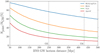 |
Fig. 6. Fraction of BNS mergers that will be detectable both in GWs and through their radio afterglow (Njoint) vs. those only detectable in GWs (NGW). The mergers are simulated up to the horizon of aLIGO Hanford with the dashed vertical lines indicating the sensitivities in O3 and O4. SKA2 or ngVLA, SKA1, VLA, and Apertif are shown as the blue, orange, green, and red curves, respectively. During O4, Apertif will be able to detect ∼11% of the well-localised GW events. |
5.4. Monte Carlo simulation
Our results from the Monte Carlo simulation for the observatories besides Apertif are nearly identical to Duque et al. (2019), confirming our methods. Future observatories such as SKA1, SKA2, or ngVLA, which are not yet operational during O4, could be sensitive enough to facilitate population level studies of BNS afterglows. They pose great promise in future observing runs. If they were operational during O4 already, SKA1 would detect 34% of the well-localised events with SKA2 detecting almost two-thirds of the events at 64% coverage.
From the telescopes that will be operational during O4, Apertif will be able to detect roughly a third of the afterglows that SKA1 would detect. This is ∼11% of the well-localised GW events. The VLA will be able to detect ∼19% of the same events. While Apertif is certainly less sensitive than the VLA, the criterion of Eq. (3) does not take into account the FOV of the different arrays. In this regard, Apertif has an advantage over the VLA. Hence, for events with bigger localisation regions it could be that Eq. (3) is not met, impeding a VLA observation of the afterglow, whereas Apertif might still be able to make a detection. Furthermore, even if Eq. (3) is met, the localisation region may still only be tractable for follow-up by large FOV telescopes. Previous GW detections by only two detectors have shown large localisation regions in the past (Fig. 5 of Abbott et al. 2020b), but we note that optical/infrared follow-up could also be crucial for localising such events.
Half of the BNS events in O4 will likely have a localisation that is small enough to be followed up with Apertif. The median 90% credible localisation region is just 33 deg2 (Abbott et al. 2020b), or about four Apertif pointings if the shape matches. From the expected BNS events in O4 and the results presented above, it follows that up to three afterglows will be detectable by Apertif. In the optimistic scenario that all events will have either a small localisation region or are localised through, for example optical or infrared follow-up, this number doubles. Moreover, for the afterglows that have not been observed in optical or infrared wavelengths, for example for the large fraction that happen in the day-time sky, wide field radio telescopes such as Apertif may be the only way to detect the EM signal at all.
As a final point, we emphasise the need for regular radio follow-up of the BNS merger. The radio criterion used in these simulations only looks at the detectability of the afterglow. This does not necessarily translate into an actual detection if the emission flux density is close to the sensitivity limit of the telescope (this is also discussed in Duque et al. 2019). The forecasts given in this section should therefore be seen as an upper limit. Even so, multiple marginal detections would still have significant scientific potential and should be actively pursued.
6. Conclusions
In this work, we have described the first follow-up of a BNS merger with the new Apertif PAFs installed on the WSRT. We covered an 9.5 deg2 region of high probability in the localisation sky map of the first O3 BNS event, GW190425, over three observational epochs. While we only observed a small fraction of the approximate 7500 deg2 90% credible localisation region, a possible counterpart could have been of high scientific significance. We identified 5 candidate counterparts based on their flux variability in our observations. As we found no associated host galaxies for either of the sources at a luminosity distance consistent with GW190425, we ruled them all out. We also looked for possible counterparts in transient sources with only one flux measurement. Our initial analysis found 55 such candidate transients. These were all determined to be imaging artefacts after manual inspection. Although we did not find a radio afterglow counterpart to GW190425, this search helped develop the pipeline and methods that will be instrumental for future searches of radio afterglows with Apertif. Furthermore, the average sensitivity that will be achieved in future observations for finding BNS afterglows will increase with further characterisation and commissioning of Apertif.
We also made predictions for our ability to detect BNS merger afterglows in the fourth observing run of the GW detector network. We extended simulations from Duque et al. (2019) by including Apertif and estimate that up to three afterglows will be detectable by the telescope. While the sensitivity of Apertif is lower than other radio telescopes, it has a significant advantage in terms of FOV. We caution that considerable uncertainties remain in the GW localisation array as well as the BNS population distribution.
Acknowledgments
We thank Antonia Rowlinson, Mark Kuiack and Kelly Gourdji for the helpful discussions and suggestions about TraP. We thank David Gardenier for a helpful discussion about the Monte Carlo simulations. We thank the anonymous referee for their thoughtful comments which have certainly improved this work. This research was supported by Vici research program ‘ARGO’ with project number 639.043.815, financed by the Dutch Research Council (NWO). J.V.L., Y.M., L.C.O. and R.S. furthermore acknowledge funding from the European Research Council under the European Union’s Seventh Framework Programme (FP/2007-2013)/ERC Grant Agreement No. 617199 (‘ALERT’), while JMvdH acknowledges ERC funding from (FP/2007-2013)/ERC Grant Agreement No. 291531 (‘HIStoryNU’). EAKA is supported by the WISE research programme, which is financed by NWO. DV acknowledges support from the Netherlands eScience Center (NLeSC) under grant ASDI.15.406. We make use of data from the Apertif system installed at the Westerbork Synthesis Radio Telescope owned by ASTRON. ASTRON, The Netherlands Institute for Radio Astronomy, is an institute of NWO.
References
- Aasi, A. J., Abbott, B. P., Abbott, R., et al. 2015, CQG, 32, 074001 [Google Scholar]
- Abbott, B. P., Abbott, R., Abbott, T. D., et al. 2017, ApJ, 848, L13 [NASA ADS] [CrossRef] [Google Scholar]
- Abbott, R., Abbott, T. D., Abraham, S., et al. 2020a, ArXiv e-prints [arXiv:2010.14527] [Google Scholar]
- Abbott, B. P., Abbott, R., Abbott, T. D., et al. 2020b, ApJ, 892, L3 [Google Scholar]
- Abbott, B. P., Abbott, R., Abbott, T. D., et al. 2020c, Liv. Rev. Rel., 23, 3 [CrossRef] [Google Scholar]
- Acernese, F., Agathos, M., Agatsuma, K., et al. 2014, CQG, 32 [Google Scholar]
- Adams, E. A. K., & van Leeuwen, J. 2019, Nat. Astron., 3, 188 [NASA ADS] [CrossRef] [Google Scholar]
- Alexander, K. D., Berger, E., Fong, W., et al. 2017, ApJ, 848, L21 [NASA ADS] [CrossRef] [Google Scholar]
- Beniamini, P., Nava, L., & Piran, T. 2016, MNRAS, 461, 51 [NASA ADS] [CrossRef] [Google Scholar]
- Chornock, R., Berger, E., Kasen, D., et al. 2017, ApJ, 848, L19 [NASA ADS] [CrossRef] [Google Scholar]
- Condon, J. J., Cotton, W. D., Greisen, E. W., et al. 1998, AJ, 115, 1693 [NASA ADS] [CrossRef] [Google Scholar]
- Coughlin, M. W., Ahumada, T., Anand, S., et al. 2019, ApJ, 885, L19 [NASA ADS] [CrossRef] [Google Scholar]
- Coulter, D. A., Foley, R. J., Kilpatrick, C. D., et al. 2017, Science, 358, 1556 [NASA ADS] [CrossRef] [Google Scholar]
- de Ruiter, H. R., Willis, A. G., & Arp, H. C. 1977, A&AS, 28, 211 [NASA ADS] [Google Scholar]
- Dobie, D., Stewart, A., Murphy, T., et al. 2019, ApJ, 887, L13 [CrossRef] [Google Scholar]
- Duque, R., Daigne, F., & Mochkovitch, R. 2019, A&A, 631, A39 [CrossRef] [EDP Sciences] [Google Scholar]
- Dálya, G., Galgóczi, G., Dobos, L., et al. 2018, MNRAS, 479, 2374 [Google Scholar]
- Fender, R., Stewart, A., Macquart, J. P., et al. 2015, Advancing Astrophysics with the Square Kilometre Array (AASKA14), 51 [CrossRef] [Google Scholar]
- Gendre, B., Lachaud, C., Adya, V., et al. 2019, GRB Coordinates Network, 24673 [Google Scholar]
- Ghirlanda, G., Salafia, O. S., Pescalli, A., et al. 2016, A&A, 594, A84 [NASA ADS] [CrossRef] [EDP Sciences] [Google Scholar]
- Ghirlanda, G., Salafia, O. S., Paragi, Z., et al. 2019, Science, 363, 968 [NASA ADS] [CrossRef] [Google Scholar]
- Haggard, D., Nynka, M., Ruan, J. J., et al. 2017, ApJ, 848, L25 [NASA ADS] [CrossRef] [Google Scholar]
- Hallinan, G., Corsi, A., Mooley, K. P., et al. 2017, Science, 358, 1579 [NASA ADS] [CrossRef] [Google Scholar]
- Hotokezaka, K., Nissanke, S., Hallinan, G., et al. 2016, ApJ, 831, 190 [NASA ADS] [CrossRef] [Google Scholar]
- LIGO Scientific Collaboration & Virgo Collaboration 2017, Phys. Rev. Lett., 119, 161101 [NASA ADS] [CrossRef] [PubMed] [Google Scholar]
- LIGO Scientific Collaboration & Virgo Collaboration 2019, Phys. Rev. X, 9, 031040 [Google Scholar]
- Mohan, N., & Rafferty, D. 2015, Astrophysics Source Code Library [record ascl:1502.007] [Google Scholar]
- Mooley, K. P., Frail, D. A., Ofek, E. O., et al. 2013, ApJ, 768, 165 [NASA ADS] [CrossRef] [Google Scholar]
- Mooley, K. P., Frail, D. A., Dobie, D., et al. 2018a, ApJ, 868, L11 [Google Scholar]
- Mooley, K. P., Deller, A. T., Gottlieb, O., et al. 2018b, Nature, 561, 355 [Google Scholar]
- Nakar, E., Piran, T., & Granot, J. 2002, ApJ, 579, 699 [NASA ADS] [CrossRef] [Google Scholar]
- Offringa, A. R., de Bruyn, A. G., Biehl, M., et al. 2010, MNRAS, 405, 155 [NASA ADS] [Google Scholar]
- Offringa, A. R., Gronde, J. J. v. d., & Roerdink, J. B. T. M. 2012, A&A, 539, A95 [NASA ADS] [CrossRef] [EDP Sciences] [Google Scholar]
- Offringa, A., Mckinley, B., Hurley-Walker, N., et al. 2014, MNRAS, 444, [Google Scholar]
- Oosterloo, T., Verheijen, M., & van Cappellen, W. 2010, 43 ISKAF2010 Science Meeting Place: ArXiv e-prints [arXiv:1007.5141] [Google Scholar]
- Rowlinson, A., Stewart, A. J., Broderick, J. W., et al. 2019, Astron. Comput., 27, 111 [CrossRef] [Google Scholar]
- Sarbadhicary, S. K., Tremou, E., Stewart, A. J., et al. 2020, ApJ, submitted, [arXiv: 2009.05056] [Google Scholar]
- Selina, R. J., Murphy, E. J., McKinnon, M., et al. 2018, in Ground-based and Airborne Telescopes VII, International Society for Optics and Photonics, 10700, 107001O [Google Scholar]
- Somiya, K. 2012, CQG, 29 [Google Scholar]
- Swinbank, J. D., Staley, T. D., Molenaar, G. J., et al. 2015, Astron. Comput., 11, 25 [CrossRef] [Google Scholar]
- The KAGRA Collaboration, 2013, Phys. Rev. D, 88 [Google Scholar]
- van Diepen, G., Dijkema, T. J., & Offringa, A. 2018, Astrophysics Source Code Library [record ascl:1804.003] [Google Scholar]
- Veitch, J., Raymond, V., Farr, B., et al. 2015, Phys. Rev. D, 91, 042003 [NASA ADS] [CrossRef] [Google Scholar]
Appendix A: Distribution of variability statistics
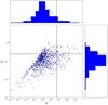 |
Fig. A.1. Histogram of the two-dimensional distribution of the variability statistics η and V calculated by TraP for each source with two or three flux density measurements in our three epochs of observation. |
All Tables
Overview of the five candidate variables found in our observations with flux measurements consistent with the expected afterglow emission of GW190425.
All Figures
|
Fig. 1. Part of the LIGO/Virgo localisation sky map on the northern hemisphere for GW190425. The full sky map has a 90% credible sky area of 7461 deg2, which reduces to 1378 deg2 at the 50% level. The blue contour encompasses the 50% credible sky area on this part of the sky. The inset shows the approximate Apertif FOV in yellow. |
| In the text | |
|
Fig. 2. Apertif mosaic, centred on 16:25:12.0, 17:47:24.0, covering a region of high probability in the localisation skymap of GW190425. The mosaic, our third epoch, was observed 109 days post merger. |
| In the text | |
|
Fig. 3. Integrated flux vs. absolute value of relative difference in flux Δfx, y, defined in Eq. (1). This is calculated for epochs 1 and 2 (blue circles), epochs 1 and 3 (pink diamonds), and epochs 2 and 3 (orange crosses). The scatter is larger than what could be expected in terms of rms noise error with median values of Δf1, 2, Δf1, 3, and Δf2, 3 of 13.7%, 10.6%, and 8.9%, respectively. |
| In the text | |
|
Fig. 4. Continuum image for beam “00” of epoch 2 made with Apercal (left) and manually reprocessed (right, see text for details). Image quality is improved in the reprocessed image with better side lobe suppression of the central bright source and less visible rings from direction-dependent errors. |
| In the text | |
|
Fig. 5. Fit to radio light curve of afterglow of GW170817 (Mooley et al. 2018a) in blue. The curve is plotted on a log-log scale to easily show the power-law dependence. The 3σ Apertif design sensitivity is shown in black. Three observations on the same days post merger as our observations for GW190425 are shown as orange stripes. |
| In the text | |
|
Fig. 6. Fraction of BNS mergers that will be detectable both in GWs and through their radio afterglow (Njoint) vs. those only detectable in GWs (NGW). The mergers are simulated up to the horizon of aLIGO Hanford with the dashed vertical lines indicating the sensitivities in O3 and O4. SKA2 or ngVLA, SKA1, VLA, and Apertif are shown as the blue, orange, green, and red curves, respectively. During O4, Apertif will be able to detect ∼11% of the well-localised GW events. |
| In the text | |
|
Fig. A.1. Histogram of the two-dimensional distribution of the variability statistics η and V calculated by TraP for each source with two or three flux density measurements in our three epochs of observation. |
| In the text | |
Current usage metrics show cumulative count of Article Views (full-text article views including HTML views, PDF and ePub downloads, according to the available data) and Abstracts Views on Vision4Press platform.
Data correspond to usage on the plateform after 2015. The current usage metrics is available 48-96 hours after online publication and is updated daily on week days.
Initial download of the metrics may take a while.