| Issue |
A&A
Volume 651, July 2021
|
|
|---|---|---|
| Article Number | A48 | |
| Number of page(s) | 10 | |
| Section | Interstellar and circumstellar matter | |
| DOI | https://doi.org/10.1051/0004-6361/202140550 | |
| Published online | 12 July 2021 | |
Compact disks
An explanation to faint CO emission in Lupus disks★
1
European Southern Observatory,
Karl-Schwarzschild-Str 2,
85748
Garching,
Germany
e-mail: This email address is being protected from spambots. You need JavaScript enabled to view it.
2
Leiden Observatory, Leiden University,
PO Box 9513,
2300
RA Leiden,
The Netherlands
3
School of Physics and Astronomy, University of Leicester,
Leicester
LE1 7RH,
UK
4
NASA Headquarters,
300 E Street SW,
Washington,
DC
20546,
USA
5
Institute for Astronomy, University of Hawai’i at Manoa,
Honolulu,
HI,
USA
6
Max-Planck Institut für Extraterrestrische Physik (MPE),
Giessenbachstr. 1,
85748
Garching,
Germany
Received:
12
February
2021
Accepted:
27
April
2021
Abstract
Context. ALMA disk surveys have shown that a large fraction of observed protoplanetary disks in nearby star-forming regions (SFRs) are fainter than expected in CO isotopolog emission. Disks not detected in 13CO line emission are also faint and often unresolved in the continuum emission at an angular resolution of around 0.2 arcsec.
Aims. Focusing on the Lupus SFR, the aim of this work is to investigate whether this population comprises radially extended and low-mass disks – as commonly assumed so far – or intrinsically radially compact disks, an interpretation that we propose in this paper. The latter scenario was already proposed for individual sources or small samples of disks, while this work targets a large population of disks in a single young SFR for which statistical arguments can be made.
Methods. We ran a new grid of physical–chemical models of compact disks with the physical–chemical code DALI in order to cover a region of the parameter space that has not been explored before with this code. We compared these models with 12CO and 13CO ALMA observations of faint disks in the Lupus SFR, and report the simulated integrated continuum and CO isotopolog fluxes of the new grid of compact models.
Results. Lupus disks that are not detected in 13CO emission and have faint or undetected 12CO emission are consistent with compact disk models. For disks with a limited radial extent, the emission of CO isotopologs is mostly optically thick and scales with the surface area, that is, it is fainter for smaller objects. The fraction of compact disks is potentially between roughly 50% and 60% of the entire Lupus sample. Deeper observations of 12CO and 13CO at a moderate angular resolution will allow us to distinguish whether faint disks are intrinsically compact or extended but faint, without the need to resolve them. If the fainter end of the disk population observed by ALMA disk surveys is consistent with such objects being very compact, this will either create a tension with viscous spreading or require MHD winds or external processes to truncate the disks.
Key words: protoplanetary disks / submillimeter: planetary systems
Full Tables B.2 and B.3 are only available at the CDS via anonymous ftp to cdsarc.u-strasbg.fr (130.79.128.5) or via http://cdsarc.u-strasbg.fr/viz-bin/cat/J/A+A/651/A48
© ESO 2021
1 Introduction
Thanks to its exquisite angular resolution and unprecedented sensitivity, the Atacama Large Millimeter/submillimeter Array (ALMA) has revolutionized the field of star and planet formation. Together with the very popular high-angular-resolution images (see e.g., ALMA Partnership 2015; Andrews et al. 2018), ALMA has also significantly enhanced the disk sample size by surveying disks at moderate resolution in many different nearby star-forming regions (SFRs). Both dust and gas components have been traced through submillimeter (submm) continuum and CO isotopolog rotational line emission in the Lupus, Chamaeleon I, Orion Nebula Cluster, Ophiuchus, IC348, Taurus, and Corona Australis, σ-Orionis, λ-Orionis, and Upper Scorpius regions (Ansdell et al. 2016, 2017, 2020; Pascucci et al. 2016; Eisner et al. 2016; Cieza et al. 2019; Long et al. 2018; Cazzoletti et al. 2019; Barenfeld et al. 2016), which are regions of between ~1 and ~10 Myr old. Most of the disks in the SFRs targeted by ALMA have also been observed in the optical with spectroscopy in order to constrain their stellar properties and mass accretion rates (see e.g., Herczeg & Hillenbrand 2014; Alcalá et al. 2017; Manara et al. 2017, 2020).
One of the main results of these surveys, unfortunately carried out with short integration times, is that the dust continuum and CO isotopologs emission is fainter than expected leading to measurements of low dust and gas masses (Ansdell et al. 2016; Pascucci et al. 2016; Long et al. 2017; Miotello et al. 2017; Manara et al. 2018). Another peculiar aspect of the surveyed disks is that the fainter part of the disk population often shows compact unresolved continuum emission and is not detected in CO isotopologs (see e.g., Long et al. 2018; Barenfeld et al. 2016; Piétu et al. 2014). Whether the observations only reveal the tip of a faint extended emission or these disks are intrinsically compact is still not constrained by available data. Nevertheless, it is critical to distinguish between these opposite scenarios because of the implications on disk evolution. Viscous evolution would in fact predict large gaseous disks, and, in contrast, small outer radii could be explained by magneto-centrifugal (MHD) winds or external processes that truncate the disks (see e.g., Clarke & Pringle 1991; Clarke et al. 2007; Vincke et al. 2015; Rosotti & Clarke 2018; Lesur 2020; Sellek et al. 2020; Trapman et al. 2020; Zagaria et al., in prep.).
Disks around binary stars represent a category of sources that are expected to have a smaller radial extent due to the interaction between the two disks. Some recent works have focused on the continuum emission of disks around binary systems and have shown that such disks extend to smaller radii than the population of disks around single stars, reflecting theoretical predictions (Manara et al. 2019; Zurlo et al. 2020).
The idea that disks with faint CO fluxes may be radially compact is not new. Barenfeld et al. (2016) proposed that an explanation for the lack of CO detections in approximately half of the disks with detected continuum emission is that CO is optically thick but has a compact emitting area (< 40 au). A similar result was found with IRAM Plateau de Bure observations of T Tauri disks by Piétu et al. (2014), which showed that faint continuum and CO emission in disks often seems to be associated with more compact disks that still have high surface densities in their inner regions. Piétu et al. (2014) also argued that this type of sources could represent upto 25% of the whole disk population. Furthermore, Hendler et al. (2017) show that the unexpectedly faint [OI] 63 μm emission of very low-mass stars (VLMSs) observed with the Herschel Space Observatory PACS spectrometer is likely indicative of smaller disk sizes than previously thought. Also, source-specific models based on CO upper limits also show that some disks need to be compact in size in order to explain their CO nondetections (Woitke et al. 2011; Boneberg et al. 2018). Finally, a recent CN study carried out in the entire Lupus sample showed that, for many of the targeted disks, and importantly the ones that also show faint CO fluxes, the critical radius Rc must be small, even less than 15 au, in order to reproduce the observed low CN fluxes (van Terwisga et al. 2019).
In contrast with these findings, the physical–chemical disk models run with DALI that were employed to interpret the observationsfrom the Lupus and Chameleon disk surveys were originally tailored to larger and brighter disks (Miotello et al. 2016, 2017; Long et al. 2017). A set of more representative DALI models for the fainter and possibly more compact disks was missing but needed for a better understanding of the existing population of fainter disks, as also recently noted by Trapman et al. (2021); such a set is presented in Sect. 3. The simulated fluxes are compared with observations of the faint disks in the Lupus SFR (63 out of 99 sources, presented in Sect. 2) and the fraction of potentially compact disks is quantified and discussed in Sects. 4 and 5. Finally, the simulated integrated continuum and CO isotopolog fluxes of the new grid of compact disk models are reported in Appendix Bas a new instrument for the interpretation of current and future ALMA observations of disks with faint CO emission.
2 ALMA observations
For this work, we use ALMA Band 6 observations of the continuum and CO isotopolog emission of disks in the Lupus SFR (see Ansdell et al. 2018, for more details). More specifically, we focus on the sources that have not been detected in 13CO (J = 2−1) emission and whose 12CO (J = 2−1) luminosity is lower than 2.5 × 10¹⁸ mJy km s−1 pc2. Applying this cut in 12CO (J = 2−1) luminosity, we exclude the brighter and resolved disks where CO outer radii were measured by Ansdell et al. (2018). Their CO isotopolog fluxes can in fact be explained by physical–chemical models of viscously evolving disks (Trapman et al. 2020). Finally, our sample of faint Lupus disks comprises 63 disks, of which only 10 have 12CO (J = 2−1) detections (see Table B.1).
The integrated 12CO and 13CO (J = 2−1) line luminosities are presented in Fig. 1 as black squares, where 3σ 13CO and 12CO upper limits, calculated as three times the rms using an aperture equal to the size of the typical beam (i.e., ~ 0.21″–0.25″, equivalent to ~ 30–40 au at 160 pc), which assumes that the disk is only emitting within the beam, are shown by black and gray arrows, respectively (Ansdell et al. 2018). Previously unpublished 12CO fluxes together with the 13CO and 12CO upper limits of the selected sample of Lupus disks are reported in Table B.1. Some level of cloud absorption affects a few of the Lupus sources considered in this work (see 12CO spectra in Fig. 11 of Ansdell et al. 2018), whose line luminosities are shown by the empty squares in Fig. 1. Finally, 12CO and 13CO nondetections are shown as upper limits, calculated as three times the rms, and shown as gray arrows. The line luminosities1 are calculated using the distance of each single object measured by Gaia DR2 (Gaia Collaboration 2018; Alcalá et al. 2019).
The stellar luminosity L⋆ and stellar mass M⋆ of the selected sources, obtained using the evolutionary track by Baraffe et al. (2015), are reported in Table B.1 (Alcalá et al. 2017). Many of these sources can be classified as VLMSs, with M⋆ ≲ 0.3 M⊙ (Liebert & Probst 1987). Almost all sources that are detected in 12CO are instead T Tauri-like stars.
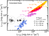 |
Fig. 1 Lupus 12CO and 13CO (J = 2− 1) line luminosity are presented with black squares (empty squares if the 12CO line is partially absorbed by the cloud), where the 13CO nondetections are shown as upper limits by the black arrows and the 12CO (and 13CO) nondetections are shown as upper limits by the gray arrows. We note that the 3σ upper limits are calculated using an aperture equal to the size of the typical beam (i.e., ~ 0.21–0.25″, equivalent to~30–40 au at 160 pc; see Ansdell et al. 2018). DALI model results from Miotello et al. (2016) are shown with filled circles, color-coded by disk mass. Different symbol sizes represent different values of the critical radius Rc. |
3 Models
Inspired by the observations presented in Sect. 2, we designed a grid of compact disk physical-chemical models. We use the code DALI (Dust And LInes, Bruderer et al. 2012) with a similar setup as in Miotello et al. (2016). The disk surface density distribution is parametrized by a power-law function, following the prescription proposed by Andrews et al. (2011):
![Mathematical equation: \begin{equation*} \Sigma_{\textrm{gas}}=\Sigma_{\textrm{c}}\left(\frac{R}{R_{\textrm{c}}}\right)^{-\gamma} \exp \left[-\left(\frac{R}{R_{\textrm{c}}}\right)^{2-\gamma}\right], \end{equation*}](/articles/aa/full_html/2021/07/aa40550-21/aa40550-21-eq1.png) (1)
(1)
where Rc is the so-called critical radius. In the large grid of T Tauri-like disk models presented by Miotello et al. (2016), Rc was set to 30, 60, and 200 au, and the power-law index γ to 0.8, 1, and 1.5, resulting in disks with non-negligible surface density up to several hundreds of astronomical units (au; see right panels of Fig. B.1). Such models are not representative of compact disks such as those considered in this work, which show unresolved or marginally resolved continuum emission at a resolution of 36 au (18 au in radius).
For this study, the disk radial extent has been drastically reduced by setting Rc to 0.5, 1, 2, 5, and 15 au, and γ to 0.5, 1.0, and 1.5. The other disk parameters are also listed below for completeness: disk mass Mdisk = 10−5, 10−4, 10−3, 10−2 M⊙; scale height h = 0.1; flaring angle ψ = 0.1; large-over-small grain mass fraction is flarge = 0.9, and settling parameter χ = 0.2 (see Table 1). Two sets of models were run to cover different stellar parameters. First, T Tauri-like disk models were run, where the stellar spectrum is composed of a black body with a temperature Teff = 4000 K and a UV excess that mimics a mass accretion rate of 10−8 M⊙ yr−1, and the stellar luminosity and mass are set to L⋆ = 1 L⊙ and M⋆ = 1.1 M⊙ as in Miotello et al. (2016). As most of the fainter disks observed with ALMA orbit low-mass and low-luminosity young stars, the second set of models uses a synthetic stellar spectrum more representative of the observed stellar parameters. More precisely, the spectrum is composed of a black body with a temperature Teff = 3400 K and a UV excess that mimics a mass accretion rate of 10−9 M⊙ yr−1. The stellar luminosity and mass are set to L⋆ = 0.16 L⊙ and M⋆ = 0.26 M⊙. Hereafter, we refer to these as VLMS-like disk models. We also account for the interstellar UV radiation field (Draine 1978) and the cosmic microwave background as external sources of radiation. We also consider cosmic rays as a source of ionization (see e.g., Bosman et al. 2018; Trapman et al. 2021, and references therein), for which a rate of ζCR = 5 × 10¹⁷ s−1 is adopted.
4 Results
Extended disk models previously run with DALI (Dust And LInes, Bruderer et al. 2012) by Miotello et al. (2016) with ISM-like volatile C and O abundances may not always be able to simultaneously reproduce 12CO and 13CO emission of the observed CO-faint disks in Lupus. This is shown in Fig. 1, where such models are presented with colored circles and the observations are reported in black and gray.
The CO-faint disks in Lupus can be divided in two subsamples, highlighted with two ellipses in Fig. 1. The group A is composed of 11 disks, mostly detected in 12CO, with line luminosity 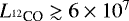 mJy km s−1 pc2. Two objects in this group are instead not detected either in 12CO or in 13CO. Disks in group A are consistent with the 10−5 M⊙ extended disk models, shown by the blue symbols in Fig. 1.
A second set of 52 disks, group B, is composed of disks that are not detected either in 13CO or in 12CO, shown by the gray arrows (except for one 12CO detection, shown by the black square). These are more extreme cases that are not compatible with any of the models by Miotello et al. (2016). Accordingly, Miotello et al. (2017) needed to assume high levels of volatile carbon and oxygen depletion as a solution for reaching fainter CO fluxes and match the observed line luminosity.
In Fig. 2, the results of our new grid of compact disk models are shown with colored circles in comparison with the observations of the subsample of Lupus disks studied in this work. Disk masses are color coded, while different values of Rc are shown by different symbol sizes. Compact disk models, with Rc smaller than 15 au, produce integrated 12CO and 13CO line luminosities that are compatible with Lupus disks in group B, and most sources in group A. Overall, there is no significant difference between the CO luminosities simulated with T Tauri (panel a) and those with VLMSs models (panel b), but the former are somewhat higher than the latter. This behavior is caused by the fact that 12CO emission is substantially optically thick as the column density reaches very high values in compact disks. Under the optically thick approximation, the intensity of the emission scales directly with the temperature of the emitting material, and it is therefore expected that T Tauri-like disk models reach higher luminosity than VLMS-like disk models with the same disk parameters. Such an effect is also seen for 13CO integrated line luminosities, which are generally higher for T Tauri-like disk models. Even 13CO emission is mostly optically thick in compact disk models: in fact 12CO and 13CO integrated line luminosities scale almost linearly as shown in Fig. 2. Miotello et al. (2016) are able to fit integrated line luminosity to simple formulae: in extended disk models, 13CO emission scales directly with disk mass for Mdisk < 2 × 10⁻⁴ M⊙ and can be used as a tracer of disk mass. On the contrary, for compact disk models 13CO does not scale linearly with mass, even for the lower mass disk models. This is in line with the findings of Boneberg et al. (2018) and Greenwood et al. (2017), who, using thermochemical modeling of brown dwarf (BD) disks, show that CO observations of compact disks are insensitive to disk mass because of the high optical depths. Optically thinner tracers, such as C18O, are therefore needed to trace disk mass. Also, for this new grid of models, 13CO and C18O line luminosities can be fitted to a logarithmic function, as reported in more detail in Appendix A.
Another consequence of the optically thick approximation is that luminosity directly scales with the surface area of the emitting material, linking the observed integrated luminosity to the disk radial extent. This trend is found in thesimulated luminosity and shown in Fig. 2. For each disk-mass bin, models with larger Rc (larger symbols) show higher 12CO and 13CO line luminosity than models with smaller Rc (smaller symbols), independent of the stellar properties. A similar trend was also found for more extended disk models (see Fig. 1), but the increase in luminosity due to larger critical radii was modest, as the emission was mostly optically thin, especially for disks with masses smaller than 10−3 M⊙.
Finally, 12CO and 13CO (J = 2−1) integrated line luminosities are shown for compact (Rc ≤ 15 au, this work) and extended (Rc ≥ 30 au, Miotello et al. 2016)disk models in Fig. 3. The two sets of models cover different regions of the luminosity–luminosity space, with more extended disk models resulting in higher 12CO and 13CO integrated line luminosities. The dotted gray line in Fig. 3 shows the median of the 13CO upper limits (Ansdell et al. 2018). As discussed above, the simulated 13CO and 12CO emission obtained with compact disk models is optically thick. Similar conditions are also found for very massive extended disk models, that is, with disk masses larger than 10−3 M⊙. The extended disk models with Mdisk = 10−2 M⊙, shown with the large yellow symbols produce 12CO and 13CO integrated line luminosity which qualitatively follows the same trend as the compact disk model results (small symbols). On the other hand, 13CO emission of less massive extended disk models deviates from the optically thick regime, bending to a steeper trend, because 13CO optically thinner emission scales more directly with disk mass.
When comparing the sample of faint Lupus disks considered in this work and the model results presented in Fig. 3, it is clear that by improving in sensitivity, that is, by re-observing the faintest disks, which were not detected in 12CO or 13CO, for longer integration times, it would be possible to discriminate between the two scenarios: low-mass extended disks versus compact disks. This would be especially interesting for the disks in group A, as it is not possible to use current observations to decipher whether they are compact or extended, but with very low CO surface density.
Parameters of the disk models.
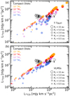 |
Fig. 2 Lupus 12CO and 13CO (J = 2−1) line luminosity are presented with black squares (empty squares if the 12CO line is partially absorbed by the cloud), where the 13CO nondetections are shown as upper limits by the black arrows and the 12CO (and 13CO) nondetections are shown as upper limits by the gray arrows. DALI model results for T Tauri disk models are shown in panel a, and those for VLMS disk models in panel b with filled circles, color-coded by disk mass. Different symbol sizes represent different values of the critical radius Rc. The scales are different from those in Fig. 1. |
5 Discussion
The compact disk models presented in this paper complement the large grid of extended models published by Miotello et al. (2016), filling a new part of the parameter space that had previously not been extensively sampled by DALI models. As shown in Fig. 2, such new models are consistent with ALMA observations of the fainter disks in the Lupus SFR (Ansdell et al. 2018) and could provide a simple solution to the problem of faint CO isotopolog emission in disks.
Faint CO isotopolog observations of disks have recently been interpreted as a sign of quick chemical evolution. This hypothesis is supported by Herschel-PACS observations of the HD fundamental line in a few bright disks. These observations showed that CO-based gas masses can be order(s) of magnitude smaller than HD-based disk masses (e.g., Bergin et al. 2013; Favre et al. 2013). This potential inconsistency has been explained by locking up of volatiles as ice in larger bodies, leading to low observed CO fluxes, and this is supported by observations and modeling of other molecular species such as C2 H and N2 H+ (see e.g., Cleeves et al. 2018; Miotello et al. 2019; Anderson et al. 2019; Fedele & Favre 2020, and references therein). It is still unclear whether or not such a scenario, which was tested uniquely for bright and extended disks, also applies in the case of compact disks, but it is not, in principle, in conflict with the results presented in Sect. 4. However, chemical models require the presence of an icy midplane in order to efficiently lock C and O in less volatile species (see e.g., Eistrup et al. 2016, 2018; Bosman et al. 2017, 2018). Compact disk models are however generally warmer and the reservoir of frozen molecular material is reduced compared to extended disk models (see Fig. B.1). If such compact disks exist, their CO isotopolog emission may therefore simply be faint because of their reduced radial size, while volatile C and O depletion may be the main factor reducing CO fluxes in more extended and colder disks.
Comparing our compact disk models with observations in Lupus allows us to constrain the fraction of disks that are potentially compact and optically thick. The entire Lupus sample studied by Ansdell et al. (2016, 2018) is composed of 99 disks, of which 11 are in group A and 52 in group B, shown in Fig. 1. Disks in group B, which represent 51.5% of the sample, are incompatible with extended disk models, unless C and O are largely depleted. Disks in group A are in principle compatible with both extended faint disks and compact thick disks. Potentially the fraction of compact disks in Lupus could be up to 62.4%, if we also consider disks in group A. To date, there are no available ALMA observations for a sample of faint Class II disks that are deep enough to discriminate between thetwo scenarios for the sources in group A, as mainly the brightest end of disks observed by the ALMA disk surveyshave been followed up at higher sensitivity and angular resolution. One-order-of-magnitude deeper 12CO and 13CO observations of faint disks at a moderate angular resolution of 0.1–0.3″, that is, reaching integrated line luminosities of ~ 2 × 10⁶ mJy km s−1 pc2 (see Fig. 3)2, will give us the opportunity to discriminate between two scenarios: very compact unresolved disks (Rc≲ 15 au) whose emission is optically thick versus extended disks whose faint optically thin emission is due to their low mass. If the sensitivity is improved by one order of magnitude, Lupus disks in group A that are already detected in 12CO will be most likely detected in 13CO, and will be compatible with both compact and extended disk models. In the latter case, their CO emission should also be resolved, which instead would not be the case if they were compatible with compact disk models. Either way, such observations would be a valuable test to our physical–chemical disk models. The potential of this approach is based on the fact that, for compact disk models, CO emission is optically thick, and the integrated flux scales with disk size. Therefore, no high-resolution observationsare needed, as one would not need to resolve the CO emission of compact disks in order to constrain their radial extent.
If the faint end of the Lupus disk population were due to very compact disks, this would challenge viscous evolution theory which would predict extended gaseous disks. Trapman et al. (2020), for example, managed to reproduce the 12CO fluxes of thebright Lupus disks with viscously evolving disk models. In their Fig. 6 they show viscous disks with initial conditions that are tuned to reproduce the average mass accretion rate in Lupus, which have observed sizes of at least ~ 100 au, that is, much more extended than what is predicted by our compact disk models. Furthermore, to consider theeffect of initial conditions more broadly, in the regime of fast viscous spreading at time t, the viscous time tν is such that tν(Rc) ~ t (Lynden-Bell & Pringle 1974; Hartmann 1998). This relation is a lower limit on Rc, because the disk could be born with an initially large size and therefore be slowly spreading. With αvisc ~ 10−3 and t ~2 Myr, this implies a Rc of at least ~ 40 au. Therefore, Rc ≲ 15 au, as in our compact disk models, implies low values of αvisc ≲ 4 × 10⁻⁴. This is at the lower end of the range of values predicted by the magneto-rotational instability. Therefore, Rc ≲ 15 au would set strong constraints on the amount of viscosity and would cast doubts on accretion being driven by viscosity rather than by an alternative mechanism such as MHD disk winds. Other processes should therefore be invoked to truncate disks to such small sizes, such as for example external photoevaporation or an encounter with another star. However, we do not expect any of these processes to be relevant in a SFR such as Lupus (see e.g., Winter et al. 2018). An interesting implication for the planet formation process is that, in such small and optically thick disks, there may be substantial reservoirs of gas for forming Jupiter-like planets within Jupiter’s orbital radius.
Irrespective of the physical interpretation, the compact disk models presented here offer a new instrument for the interpretation of current and future ALMA observations, including but not limited to those of binary disks, which extend to smaller outer radii (Manara et al. 2019; Zurlo et al. 2020; Rota et al., in prep.). The simulated integrated continuum and CO isotopolog luminosities are reported in Appendix B.
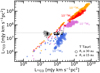 |
Fig. 3 Simulated 12CO (J = 2−1) versus 13CO (J = 2−1) line luminosity of T Tauri disk models are presented: disk masses are color-coded and different values of the critical radius Rc are shown bydifferent symbol sizes. DALI model results from this work (Rc= 0.5, 1, 2, 5, 15 au) are shown as smaller circles, while results from Miotello et al. (2016) (Rc = 30, 60, 200 au) are shown using larger symbols. Lupus 12CO and 13CO (J = 2−1) line luminosity are presented with black squares (empty squares if the 12CO line is partially absorbed by the cloud), where the 13CO nondetections are shown as upper limits by the black arrows and the 12CO (and 13CO) nondetections are shown as upper limits by the gray arrows. The dotted gray line shows the average of the 13CO Lupus upper limits. |
6 Conclusions
This paper presents results from a new grid of compact disk models with critical radii of Rc = 0.5, 1, 2, 5, 15 au, run with DALI. Our results are consistent with 12CO and 13CO fluxes of thefainter Lupus disks, which can only be explained by more extended disk models if volatile C and O are largely depleted by orders of magnitude. The main conclusions from this work are the following:
- 1.
Lupus disks that are not detected in 13CO emission, and with faint or undetected 12CO emission, may be intrinsically compact. The fraction of compact disks is potentially between roughly 50% and 60% of the entire Lupus sample;
- 2.
One-order-of-magnitude deeper 12CO and 13CO observations – compared with ALMA disk surveys observations – of faint disks at an angular resolution of 0.1–0.2″ will give us the opportunity to discriminate between two scenarios: very compact unresolved disks (Rc ≲ 15 au) whose emission is optically thick versus extended and resolved disks whose faint emission is optically thin;
- 3.
The simulated integrated continuum and CO isotopolog fluxes of the new grid of compact models are reported in Appendix B.
With this work we highlight the importance of targeting fainter disks with deep 12CO and 13CO observations, as such sources may still retain substantial reservoirs of gas for forming Jupiter-like planets. Furtehrmore, we offer a new instrument for the interpretation of current and future ALMA observations of CO-faint disks.
Acknowledgements
The authors wish to thank the anonymous referee for insightful comments and Ewine van Dishoeck, Leonardo Testi, Ted Bergin, and Antonella Natta for useful discussions. This project has received funding from the European Unions Horizon 2020 research and innovation programme under the Marie Sklodowska-Curie grant agreement no. 823823 (RISE DUSTBUSTERS). This work was funded by the Deutsche Forschungsgemeinschaft (DFG, German Research Foundation) – Ref no. FOR 2634/1 ER685/11-1. G.R. acknowledges support from the Netherlands Organisation for Scientific Research (NWO, program number 016.Veni.192.233) and from an STFC Ernest Rutherford Fellowship (grant number ST/T003855/1).
Appendix A Line intensities and disk masses
Similarly to what was done by Miotello et al. (2016, 2017), it is possible to determine how line intensities depend on disk mass by computing the medians of the 13CO and C18O (J = 2−1) line intensities obtained by the compact disk models3 (see disk parameters in Table 1) in different disk mass bins.
These trends are presented in Fig. A.1, both for 13CO (upper panel) and C18O (lower panel). Being optically thick, 13CO intensity does not increase linearly with mass, but can be fitted to a logarithmic function of the disk mass. On the contrary, C18O emission is optically thin for disk masses smaller than Mtr = 10−4 M⊙, and it scales linearly with mass. The 13CO and C18O (J = 2−1) line luminosities can be expressed by the following fit functions of the disk mass:
 (A.1)
(A.1)
and
 (A.2)
(A.2)
where Mtr,13 = 8.5 × 10⁻⁴ M⊙ and Mtr,18 = 10−4M⊙.
As 13CO emission is always optically thick in compact disk models, only C18O emission may be used as mass tracer, only if Mdisk < Mtr,18, and assuming that no volatile C and O depletion is there. The fit to the maximum and minimum simulated luminosities, shown by the gray lines in Fig. A.1, can be used to estimate uncertainties on the mass determinations, and these functions are as follows:
 (A.3)
(A.3)
and
 (A.4)
(A.4)
where Mtr,18,max = 1.8 × 10⁻⁴ and Mtr,18,min = 1.2 × 10⁻⁴.
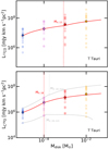 |
Fig. A.1 Median of the 13CO (upper panel) and C18O (lower panel) J = 2−1 line luminosities in different mass bins for compact disk models are presented with filled circles. Red solid lines show the fit functions presented in Eqs. (A.1) and (A.2). The translucent symbols show all model results, while the gray solid lines show the fit to the maximum and minimum luminosities, which can be used to estimate uncertainties on the mass measurements. |
Appendix B Ancillary material
The integrated 12CO (J = 2−1) fluxes for the compact disks in Lupus studied in this work are reported in Table B.1. These fluxes are measured using an aperture synthesis method, as done by Ansdell et al. (2018). For nondetections, the 3 − σ upper limitsare reported. Cloud absorption may be affecting a few of the Lupus sources considered in this work (see 12CO spectra in Fig. 11 of Ansdell et al. 2018), and integrated 12CO luminosities should be considered as meaningful lower limits. In fact, we do not expect such absorption to reduce the effective disk 12CO emission more than a factor of two.
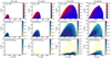 |
Fig. B.1 2D plots of the dust temperature structure, as well as the gaseous and ice CO abundance distribution for a selection of the compact T Tauri disk models: Mdisk = 10−3 M⊙, γ = 1, and Rc = 1 au (left), 2 au (middle left), 5 au (middle right), 60 au (right). We note the change of scale in the R, and Z axes in the right panels. |
The simulated spatially integrated continuum fluxes (at 880 μm in Jy) and of the CO isotopologs lines (in K km s−1) for the new grid of compact T Tauri-like and VLMS-like disk models are reported in Tables B.2 and B.3, respectively.
The 2D plots of the dust temperature structure, as well as the gaseous and ice CO abundance distribution for a selection of the compact disk models are shown in Fig. B.1. For a fixed disk mass, more compact disks are warmer than more extended disks, with Tdust higher than 20 K almost everywhere in the disk (if Rc ≤ 2 au). As a consequence the amount of CO frozen onto grains is negligible.
Simulated 12CO (J = 3−2) versus 13CO (J = 3−2) line luminosity of T Tauri disk models are presented in Fig. B.2: disk masses are color-coded and different values of the critical radius Rc are shown by different symbol sizes. DALI model results from this work (Rc= 0.5, 1, 2, 5, 15 au) are show by smaller circles, while results from Miotello et al. (2016) (Rc = 30, 60, 200 au) are shown by larger symbols.
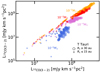 |
Fig. B.2 Simulated 12CO (J = 3−2) versus 13CO (J = 3−2) line luminosity of T Tauri disk models are presented: disk masses are color-coded and different values of the critical radius Rc are shown bydifferent symbol sizes. DALI model results from this work (Rc = 0.5, 1, 2, 5, 15 au) are shown bysmaller circles, while results from Miotello et al. (2016) (Rc = 30, 60, 200 au) are shown by larger symbols. |
12CO and 13CO fluxes and 3σ upper limits,distances (Gaia Collaboration 2018), stellar luminosity, and stellar mass (calculated using the evolutionary tracks by Baraffe et al. 2015; Alcalá et al. 2017) for the sources in the studied subsample of faint Lupus disks.
Disk parameters and integrated fluxes simulated with the grid of compact T Tauri-like models.
Disk parameters and integrated fluxes simulated with the grid of compact VLMS-like models.
References
- Alcalá, J. M., Manara, C. F., Natta, A., et al. 2017, A&A, 600, A20 [NASA ADS] [CrossRef] [EDP Sciences] [Google Scholar]
- Alcalá, J. M., Manara, C. F., France, K., et al. 2019, A&A, 629, A108 [NASA ADS] [CrossRef] [EDP Sciences] [Google Scholar]
- ALMA Partnership (Brogan, C. L., et al.) 2015, ApJ, 808, L3 [NASA ADS] [CrossRef] [Google Scholar]
- Anderson, D. E., Blake, G. A., Bergin, E. A., et al. 2019, ApJ, 881, 127 [Google Scholar]
- Andrews, S. M., Wilner, D. J., Espaillat, C., et al. 2011, ApJ, 732, 42 [Google Scholar]
- Andrews, S. M., Huang, J., Pérez, L. M., et al. 2018, ApJ, 869, L41 [Google Scholar]
- Ansdell, M., Williams, J. P., van der Marel, N., et al. 2016, ApJ, 828, 46 [Google Scholar]
- Ansdell, M., Williams, J. P., Manara, C. F., et al. 2017, AJ, 153, 240 [NASA ADS] [CrossRef] [EDP Sciences] [Google Scholar]
- Ansdell, M., Williams, J. P., Trapman, L., et al. 2018, ApJ, 859, 21 [Google Scholar]
- Ansdell, M., Haworth, T. J., Williams, J. P., et al. 2020, AJ, 160, 248 [Google Scholar]
- Baraffe, I., Homeier, D., Allard, F., & Chabrier, G. 2015, A&A, 577, A42 [NASA ADS] [CrossRef] [EDP Sciences] [Google Scholar]
- Barenfeld, S. A., Carpenter, J. M., Ricci, L., & Isella, A. 2016, ApJ, 827, 142 [Google Scholar]
- Bergin, E. A., Cleeves, L. I., Gorti, U., et al. 2013, Nature, 493, 644 [NASA ADS] [CrossRef] [PubMed] [Google Scholar]
- Boneberg, D. M., Facchini, S., Clarke, C. J., et al. 2018, MNRAS, 477, 325 [Google Scholar]
- Bosman, A. D., Bruderer, S., & van Dishoeck, E. F. 2017, A&A, 601, A36 [NASA ADS] [CrossRef] [EDP Sciences] [Google Scholar]
- Bosman, A. D., Walsh, C., & van Dishoeck, E. F. 2018, A&A, 618, A182 [NASA ADS] [CrossRef] [EDP Sciences] [Google Scholar]
- Bruderer, S., van Dishoeck, E. F., Doty, S. D., & Herczeg, G. J. 2012, A&A, 541, A91 [NASA ADS] [CrossRef] [EDP Sciences] [Google Scholar]
- Cazzoletti, P., Manara, C. F., Baobab Liu, H., et al. 2019, A&A, 626, A11 [NASA ADS] [CrossRef] [EDP Sciences] [Google Scholar]
- Cieza, L. A., Ruíz-Rodríguez, D., Hales, A., et al. 2019, MNRAS, 482, 698 [Google Scholar]
- Clarke, C. J., & Pringle, J. E. 1991, MNRAS, 249, 584 [Google Scholar]
- Clarke, C. J., Harper-Clark, E., & Lodato, G. 2007, MNRAS, 381, 1543 [Google Scholar]
- Cleeves, L. I., Öberg, K. I., Wilner, D. J., et al. 2018, ApJ, 865, 155 [NASA ADS] [CrossRef] [Google Scholar]
- Draine, B. T. 1978, ApJS, 36, 595 [NASA ADS] [CrossRef] [Google Scholar]
- Eisner, J. A., Bally, J. M., Ginsburg, A., & Sheehan, P. D. 2016, ApJ, 826, 16 [Google Scholar]
- Eistrup, C., Walsh, C., & van Dishoeck, E. F. 2016, A&A, 595, A83 [NASA ADS] [CrossRef] [EDP Sciences] [Google Scholar]
- Eistrup, C., Walsh, C., & van Dishoeck, E. F. 2018, IAU Symp., 332, 69 [Google Scholar]
- Favre, C., Cleeves, L. I., Bergin, E. A., Qi, C., & Blake, G. A. 2013, ApJ, 776, L38 [NASA ADS] [CrossRef] [Google Scholar]
- Fedele, D., & Favre, C. 2020, A&A, 638, A110 [CrossRef] [EDP Sciences] [Google Scholar]
- Gaia Collaboration (Brown, A. G. A., et al.) 2018, A&A, 616, A1 [NASA ADS] [CrossRef] [EDP Sciences] [Google Scholar]
- Greenwood, A. J., Kamp, I., Waters, L. B. F. M., et al. 2017, A&A, 601, A44 [NASA ADS] [CrossRef] [EDP Sciences] [Google Scholar]
- Hartmann, L. 1998, Cambr. Astrophys. Ser., 32 [Google Scholar]
- Hendler, N. P., Mulders, G. D., Pascucci, I., et al. 2017, ApJ, 841, 116 [Google Scholar]
- Herczeg, G. J., & Hillenbrand, L. A. 2014, ApJ, 786, 97 [Google Scholar]
- Lesur, G. 2020, Lect. Notes Ser. J. Plasma Phys., submitted [arXiv:2007.15967] [Google Scholar]
- Liebert, J., & Probst, R. G. 1987, ARA&A, 25, 473 [Google Scholar]
- Long, F., Herczeg, G. J., Pascucci, I., et al. 2017, ApJ, 844, 99 [NASA ADS] [CrossRef] [Google Scholar]
- Long, F., Pinilla, P., Herczeg, G. J., et al. 2018, ApJ, 869, 17 [NASA ADS] [CrossRef] [Google Scholar]
- Lynden-Bell, D., & Pringle, J. E. 1974, MNRAS, 168, 603 [NASA ADS] [CrossRef] [Google Scholar]
- Manara, C. F., Testi, L., Herczeg, G. J., et al. 2017, A&A, 604, A127 [NASA ADS] [CrossRef] [EDP Sciences] [Google Scholar]
- Manara, C. F., Morbidelli, A., & Guillot, T. 2018, A&A, 618, L3 [NASA ADS] [CrossRef] [EDP Sciences] [Google Scholar]
- Manara, C. F., Tazzari, M., Long, F., et al. 2019, A&A, 628, A95 [NASA ADS] [CrossRef] [EDP Sciences] [Google Scholar]
- Manara, C. F., Natta, A., Rosotti, G. P., et al. 2020, A&A, 639, A58 [CrossRef] [EDP Sciences] [Google Scholar]
- Miotello, A., van Dishoeck, E. F., Kama, M., & Bruderer, S. 2016, A&A, 594, A85 [NASA ADS] [CrossRef] [EDP Sciences] [Google Scholar]
- Miotello, A., van Dishoeck, E. F., Williams, J. P., et al. 2017, A&A, 599, A113 [NASA ADS] [CrossRef] [EDP Sciences] [Google Scholar]
- Miotello, A., Facchini, S., van Dishoeck, E. F., et al. 2019, A&A, 631, A69 [NASA ADS] [CrossRef] [EDP Sciences] [Google Scholar]
- Pascucci, I., Testi, L., Herczeg, G. J., et al. 2016, ApJ, 831, 125 [Google Scholar]
- Piétu, V., Guilloteau, S., Di Folco, E., Dutrey, A., & Boehler, Y. 2014, A&A, 564, A95 [NASA ADS] [CrossRef] [EDP Sciences] [Google Scholar]
- Rosotti, G. P., & Clarke, C. J. 2018, MNRAS, 473, 5630 [NASA ADS] [CrossRef] [Google Scholar]
- Sellek, A. D., Booth, R. A., & Clarke, C. J. 2020, MNRAS, 492, 1279 [CrossRef] [Google Scholar]
- Trapman, L., Rosotti, G., Bosman, A. D., Hogerheijde, M. R., & van Dishoeck, E. F. 2020, A&A, 640, A5 [EDP Sciences] [Google Scholar]
- Trapman, L., Bosman, A. D., Rosotti, G., Hogerheijde, M. R., & van Dishoeck, E. F. 2021, A&A 649, A95 [EDP Sciences] [Google Scholar]
- van Terwisga, S. E., van Dishoeck, E. F., Cazzoletti, P., et al. 2019, A&A, 623, A150 [NASA ADS] [CrossRef] [EDP Sciences] [Google Scholar]
- Vincke, K., Breslau, A., & Pfalzner, S. 2015, A&A, 577, A115 [NASA ADS] [CrossRef] [EDP Sciences] [Google Scholar]
- Williams, J. P., & Best, W. M. J. 2014, ApJ, 788, 59 [NASA ADS] [CrossRef] [Google Scholar]
- Winter, A. J., Clarke, C. J., Rosotti, G., et al. 2018, MNRAS, 478, 2700 [Google Scholar]
- Woitke, P., Riaz, B., Duchêne, G., et al. 2011, A&A, 534, A44 [NASA ADS] [CrossRef] [EDP Sciences] [Google Scholar]
- Zurlo, A., Cieza, L. A., Pérez, S., et al. 2020, MNRAS, 496, 5089 [Google Scholar]
Luminosities are calculated following Williams & Best (2014): L = 4πd2F, where d is the distance of the source and F is its measured spatially integrated flux.
This luminosity is set by the minimum simulated 13CO integrated flux of the 10−5 M⊙ extended disk models, i.e., 3.72 × 10⁻³ K km s−1 (see Miotello et al. 2016, for more detail).
Only for i = 10°. A similar exercise can be done for other inclination angles using the model results in Table B.2.
All Tables
12CO and 13CO fluxes and 3σ upper limits,distances (Gaia Collaboration 2018), stellar luminosity, and stellar mass (calculated using the evolutionary tracks by Baraffe et al. 2015; Alcalá et al. 2017) for the sources in the studied subsample of faint Lupus disks.
Disk parameters and integrated fluxes simulated with the grid of compact T Tauri-like models.
Disk parameters and integrated fluxes simulated with the grid of compact VLMS-like models.
All Figures
|
Fig. 1 Lupus 12CO and 13CO (J = 2− 1) line luminosity are presented with black squares (empty squares if the 12CO line is partially absorbed by the cloud), where the 13CO nondetections are shown as upper limits by the black arrows and the 12CO (and 13CO) nondetections are shown as upper limits by the gray arrows. We note that the 3σ upper limits are calculated using an aperture equal to the size of the typical beam (i.e., ~ 0.21–0.25″, equivalent to~30–40 au at 160 pc; see Ansdell et al. 2018). DALI model results from Miotello et al. (2016) are shown with filled circles, color-coded by disk mass. Different symbol sizes represent different values of the critical radius Rc. |
| In the text | |
|
Fig. 2 Lupus 12CO and 13CO (J = 2−1) line luminosity are presented with black squares (empty squares if the 12CO line is partially absorbed by the cloud), where the 13CO nondetections are shown as upper limits by the black arrows and the 12CO (and 13CO) nondetections are shown as upper limits by the gray arrows. DALI model results for T Tauri disk models are shown in panel a, and those for VLMS disk models in panel b with filled circles, color-coded by disk mass. Different symbol sizes represent different values of the critical radius Rc. The scales are different from those in Fig. 1. |
| In the text | |
|
Fig. 3 Simulated 12CO (J = 2−1) versus 13CO (J = 2−1) line luminosity of T Tauri disk models are presented: disk masses are color-coded and different values of the critical radius Rc are shown bydifferent symbol sizes. DALI model results from this work (Rc= 0.5, 1, 2, 5, 15 au) are shown as smaller circles, while results from Miotello et al. (2016) (Rc = 30, 60, 200 au) are shown using larger symbols. Lupus 12CO and 13CO (J = 2−1) line luminosity are presented with black squares (empty squares if the 12CO line is partially absorbed by the cloud), where the 13CO nondetections are shown as upper limits by the black arrows and the 12CO (and 13CO) nondetections are shown as upper limits by the gray arrows. The dotted gray line shows the average of the 13CO Lupus upper limits. |
| In the text | |
|
Fig. A.1 Median of the 13CO (upper panel) and C18O (lower panel) J = 2−1 line luminosities in different mass bins for compact disk models are presented with filled circles. Red solid lines show the fit functions presented in Eqs. (A.1) and (A.2). The translucent symbols show all model results, while the gray solid lines show the fit to the maximum and minimum luminosities, which can be used to estimate uncertainties on the mass measurements. |
| In the text | |
|
Fig. B.1 2D plots of the dust temperature structure, as well as the gaseous and ice CO abundance distribution for a selection of the compact T Tauri disk models: Mdisk = 10−3 M⊙, γ = 1, and Rc = 1 au (left), 2 au (middle left), 5 au (middle right), 60 au (right). We note the change of scale in the R, and Z axes in the right panels. |
| In the text | |
|
Fig. B.2 Simulated 12CO (J = 3−2) versus 13CO (J = 3−2) line luminosity of T Tauri disk models are presented: disk masses are color-coded and different values of the critical radius Rc are shown bydifferent symbol sizes. DALI model results from this work (Rc = 0.5, 1, 2, 5, 15 au) are shown bysmaller circles, while results from Miotello et al. (2016) (Rc = 30, 60, 200 au) are shown by larger symbols. |
| In the text | |
Current usage metrics show cumulative count of Article Views (full-text article views including HTML views, PDF and ePub downloads, according to the available data) and Abstracts Views on Vision4Press platform.
Data correspond to usage on the plateform after 2015. The current usage metrics is available 48-96 hours after online publication and is updated daily on week days.
Initial download of the metrics may take a while.