| Issue |
A&A
Volume 651, July 2021
|
|
|---|---|---|
| Article Number | A23 | |
| Number of page(s) | 11 | |
| Section | Planets and planetary systems | |
| DOI | https://doi.org/10.1051/0004-6361/202040202 | |
| Published online | 05 July 2021 | |
Influence of equilibrium tides on transit-timing variations of close-in super-Earths
I. Application to single-planet systems and the case of K2-265 b
1
Observatoire de Genève, Université de Genève,
Chemin Pegasi 51,
1290
Sauverny, Switzerland
2
Instituto de Astronomia, Geofísica e Ciências Atmosféricas, IAG-USP,
Rua do Matão 1226,
05508-900
São Paulo, Brazil
e-mail: gabrielogomes@usp.br
3
Harvard-Smithsonian Center for Astrophysics,
60 Garden Street,
Cambridge,
MA
02138, USA
Received:
22
December
2020
Accepted:
28
April
2021
With the current growth in the discovery of close-in low-mass exoplanets, recent works have been published with the aim to discuss the influences of planetary interior structure parameters on both the shape of transit light curves as well as variations in the timing of transit events of these planets. One of the main aspects explored in these works is the possibility that the precession of the argument of periapsis caused by planetary tidal interactions may lead to unique effects on the transit light curves of the exoplanets, such as the so-called transit-timing variations (TTVs). In this work, we investigate the influence of planetary tidal interactions on the transit-timing variations of short-period low-mass rocky exoplanets. For this purpose, we employed the recently developed creep tide theory to compute tidally induced TTVs. We implemented the creep tide in the recently-developed Posidonius N-body code, thus allowing for a high-precision evolution of the coupled spin-orbit dynamics of planetary systems. As a working example for the analyses of tidally induced TTVs, we applied our version of the code to the K2-265 b planet. We analyzed the dependence of tidally induced TTVs with the planetary rotation rate, uniform viscosity coefficient, and eccentricity. Our results show that the tidally induced TTVs are more significant in the case where the planet is trapped in nonsynchronous spin-orbit resonances, in particular the 3/2 and 2/1 spin-orbit resonant states. An analysis of the TTVs induced separately by apsidal precession and tidally induced orbital decay has allowed for the conclusion that the latter effect is much more efficient at causing high-amplitude TTVs than the former effect by 2–3 orders of magnitude. We compare our findings for the tidally induced TTVs obtained with Posidonius with analytical formulations for the transit timings used in previous works, and we verified that the results for the TTVs coming from Posidonius are in excellent agreement with the analytical formulations. These results show that the new version of Posidonius containing the creep tide theory implementation can be used to study more complex cases in the future. For instance, the code can be used to study multiplanetary systems, in which case planet-planet gravitational perturbations must be taken into account in addition to tidal interactions to obtain the TTVs.
Key words: planet-star interactions / planets and satellites: interiors / planets and satellites: terrestrial planets
© ESO 2021
1 Introduction
The measurement of transit-timing variations (TTVs) has been shown to be an invaluable tool in the field of exoplanetary detection and characterization (Agol et al. 2005). In multiplanet systems, for instance, the gravitational interaction between planets leads to deviations from strictly Keplerian orbits. These deviations in turn lead to a shift in the timing of planetary transit events. The TTV effects are usually investigated by directly running N-body dynamical simulations. The advantage of such an approach lies in the fact that the results are valid for arbitrary eccentricities and inclinations of the planets. Several studies have employed the technique of TTV analyses to improve the mass measurement of disturbing (and, in some cases, nontransiting) planetary companions, as well as their orbital parameters (Nesvorný & Morbidelli 2008; Lithwick et al. 2012; Nesvorný & Vokrouhlický 2016; Agol et al. 2021).
Although planet–planet interactions are among the main effects leading to high-amplitude TTVs, any interaction causing a drift of a planet from its unperturbed Keplerian orbit can induce TTVs. For very close-in planets, for instance, general relativity-induced apsidal precession and tidally induced orbital decay (see e.g., discussions in Ragozzine & Wolf 2009) may be strong enough to cause significant variations in the orbital elements of the planets and lead to observable TTVs. The detection of such TTVs caused by these disturbing forces depends on the magnitude of the induced TTVs compared to the precision of the instruments measuring transit events.
In the field of study of tidal interactions and subsequent spin-orbit evolution, the parameter which is responsible for dictating the response to tidal stress is the complex Love number, which is the ratio of the additional gravitational potential induced by the internal mass redistribution of the planet due to tidal deformation to the external tidal potential created by the perturber (Love 1911). Thus, provided that the tidally induced TTVs are big enough to be detected, matching the observed TTVs with the values estimated by numerical simulations of the tidal evolution of the system would allow us to estimate the complex Love number of the bodies, thus providing us with invaluable information regarding the interior structure of the planets and their rotational state, for example.
In a recent work, Patra et al. (2017) analyze transit and occultation data of WASP-12 b (see e.g., Hebb et al. 2009; Haswell 2018 and references therein) and show that the planet could be undergoing an orbital decay process corresponding to a mean period decay of Ṗ = −29 ± 3 ms yr−1, which would be compatible with a stellar quality factor on the order of 2 × 10⁵. However, the authors point out that apsidal precession induced by planetary tidal deformation could provide the same effects on the transit curves whencompared to the orbital decay process induced by stellar tides, in which case the Love number of the planet would be on the order of kp = 0.44 ± 0.10. The confusion between the two effects could only be solved if occultation data were analyzed in addition to transit data, in which case the contribution from apsidal precession gives an opposite sign to the occultation timing variation curves when compared to orbital decay. In a more recent work, Yee et al. (2020) analyze new transit and occultation measurements for the same system and verify that a model for the transit timings considering orbital decay is more likely to explain the TTV curve of the planet when compared to a model considering apsidal precession.
Although the recent discussions raised by Ragozzine & Wolf (2009), Patra et al. (2017), and Yee et al. (2020), for example, have paved the way for future investigations regarding the tidally induced TTVs, few studies have been dedicated to an exploration of these effects for low-mass close-in rocky exoplanets. The reason for the lack of studies for such class of exoplanets is linked to the fact that only a few of them had been discovered before the results of photometric surveys coming from missions such as Kepler (Youdin 2011; Fressin et al. 2013) and TESS (Sullivan et al. 2015). However, with the recent boom in the discovery and characterization of close-in rocky super-Earths and the improvement in the precision of the transit timing measurements, an investigation of the potential effects of planetary tidal interactions on TTVs is necessary. This may be a powerful approach at assessing the planets’ interior structure (see e.g., Bolmont et al. 2020b) as well as other parameters, such as their current rotational state, where the rotational state of the planet does indeed depend on its interior structure parameters, such as its viscosity and density.
In the field of study of tidal interactions on rocky super-Earths, several works have aimed to provide a description of the equilibrium tide and its subsequent orbital evolution scenarios by employing advanced rheological models to describe the response of these exoplanets to tidal stress (see e.g., Efroimsky 2012; Ferraz-Mello 2013; Tobie et al. 2019; Walterová & Běhounková 2020 and references therein). However, to the best of our knowledge, none of these advanced rheological models have been consistently implemented in high-precision and open-source N-body codes1, which wouldallow for a multiplanet simulation of tidally induced TTVs to a good degree of accuracy. In a recent work, Bolmont et al. (2020b) investigate the magnitude of tidally induced TTVs for the TRAPPIST-1 multiplanet system by employing the implementation of a classical approach of tidal interactions based on the constant time lag (CTL) formulation (Mignard 1979). However, this specific approach does not allow for a full exploration of the TTVs considering all the nuances of equilibrium tide interactions in rocky bodies, such as the temporary entrapment in spin-orbit resonances for moderately high values of eccentricities and planetary viscosity (see e.g., Makarov & Efroimsky 2013 and references therein). Such aspects, which are consistently reproduced using more complex rheological models, may indeed play an important role in the orbital evolution of the planets and, consequently, lead to significant changes in the tidally induced TTVs when compared to scenarios obtained by employing classical theories of equilibrium tides, such as the CTL approach.
Taking the discussions presented in Delisle et al. (2017) and Bolmont et al. (2020b) into account as well as the lack of an investigation of the topic of tidally induced TTVs using a more sophisticated tidal interaction model for the planet, we revisit, in this work, such topic in the frame of the creep tide theory (Ferraz-Mello 2013; Folonier et al. 2018). For this purpose, we implemented the tidal interactions model in the recently-developed N-body code called Posidonius2 (Blanco-Cuaresma & Bolmont 2017; Bolmont et al. 2020b).
The creep tide theory describes the response of bodies to tidal stress by supposing a Newtonian creep equation for the extended body’s shape evolution. This equation is the result of a linear approximation of the Navier-Stokes equation for a low-Reynolds-number flow (i.e., for cases where viscous forces are much more significant than inertial forces, see Ferraz-Mello 2013). We consider the formulation of the theory for homogeneous bodies whose rotation axes are perpendicular to the orbital plane (i.e., the zero-obliquity case). The equations ruling the spin and orbit evolution of the planets are shown to be easy to implement in the Posidonius code, and the response of bodies to tidal stress depends on only one parameter, which is the uniform viscosity coefficient of the body.
As a real example of a tidally induced TTV analysis, we study the K2-265 b super-Earth (Lam et al. 2018). We explore the influence of tidally induced TTVs as a function of several parameters, such as the planet’s viscosity, eccentricity, and rotational state. We also present a broad analysis of the amplitudes of tidally induced TTVs as a function of other parameters, such as the planet’s mass and radius values and its semi-major axis. Such a broad analysis allows us to identify the main parameters leading to bigger influences on the TTV values. Finally, we also provide some examples of recently-discovered systems for which tidally induced TTVs would have the highest amplitudes for a given number of transit events. Such systems are the candidates for which tidally induced TTVs can be more easily detected by the instruments measuring transit events, such as the TESS telescope.
This work is organized as follows: in Sect. 2, we present the main results of the creep tide theory which were used for the implementation in the Posidonius code and briefly give some details regarding the numerical setup used in the calculations of the TTVs. In Sect. 3, we investigate the magnitudes of tidally induced TTVs for the K2-265 b planet considering the influences of tuning the parameters presenting the most significant uncertainties in their determined values (i.e., the eccentricity, rotational state, and viscosity of the planet). We also compare the results for the TTVs obtained by using Posidonius with the ones obtained by employing some analytical approximations to generate transit timing curves. In Sect. 4, we perform a broad exploration of tidally induced TTVs as a function of both orbital and physical parameters of the star and the planet. In Sect. 5 we present the discussions of the work, and Sect. 6 summarizes our conclusions.
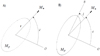 |
Fig. 1 Scheme of the geometrical setup considered in the framework of the creep tide theory, partially reproduced from Folonier et al. (2018). On the left, we have the pure static case in which the primary always points toward the companion, which is at a distance r from the primary. On the right, we have the case in which the response of the primary is delayed due to the primary’s nonzero viscosity value. In both panels,
|

2 Numerical setup
In this section, we provide the essential equations of the creep tide theory which were used in the implementation in the Posidonius code. We also present some additional information regarding the numerical integrator which provides the better precision forthe calculations of transit timing events.
2.1 The creep tide theory
The creep tide theory considers the deformations of an extended body (hereafter the primary) due to the disturbing gravitational potential due to a point-mass companion. The time evolution of the primary’s figure is described by three parameters: the equatorial deformation of the body ( ), polar oblateness (
 ), and the angle giving the orientation of the tidal bulge (δ), as it is described in the scheme in Fig. 1. These three parameters are evolved by employing a Newtonian creep equation, which is an approximate solution of the Navier-Stokes equation in the case of a low-Reynolds-number flow (see Ferraz-Mello 2013; Folonier et al. 2018 for more details).
Employing the expression for the potential of the resulting triaxial figure of the primary, we computed the forces and the torque acting on the companion. While the radial and ortho-radial components of the force (namely Fr and Fo) were used to compute the orbital evolution of the system, the reaction to the torque acting on the companion was used to compute the rotational evolution of the primary. The calculations are straightforward and they entail (Folonier et al. 2018)
![\begin{equation*} \vec{F}_{\textrm{r}}\,{=}\,\left[ -\frac{9}{10} \frac{GM_{\textrm{p}}M_{\star}R_{\textrm{p}}^2}{r^4} \mathcal{E}_{\rho} \cos 2 \delta - \frac{3}{5} \frac{GM_{\textrm{p}}M_{\star}R_{\textrm{p}}^2}{r^4} \mathcal{E}_z \right] \vec{r},\end{equation*}](/articles/aa/full_html/2021/07/aa40202-20/aa40202-20-eq3.png) (1)
(1)
![\begin{equation*} \vec{F}_{\textrm{o}}\,{=}\,\left[ \frac{3}{5} \frac{GM_pM_{\star}R_p^2}{r^4} \mathcal{E}_{\rho} \sin 2 \delta \right] (\vec{z}\,{\times}\, \vec{r}),\end{equation*}](/articles/aa/full_html/2021/07/aa40202-20/aa40202-20-eq4.png) (2)
(2)
 (3)
(3)
The unit vectors r and z × r point toward the radial and ortho-radial directions, respectively, with z being a unitvector pointing to the same direction of the orbital angular momentum vector. The parameters G, Mp, Rp, and M⋆ are the gravitational constant, mass and radius of the planet, and mass of the star, respectively.
To compute the time evolution of  ,
,  , and δ, we employed the analytical solutions for these parameters in the frame of the constant rotation rate approximation (Gomes et al. 2019), which read
![\begin{equation*} \mathcal{E}_{\rho} \cos 2 \delta\,{=}\,\bar{\epsilon}_{\rho} \sum _{k \in \mathbb{Z}} \mathcal{C}_k [\gamma \cos \phi _k - (2 \Omega - k n) \sin \phi _k],\end{equation*}](/articles/aa/full_html/2021/07/aa40202-20/aa40202-20-eq8.png) (4)
(4)
![\begin{equation*} \mathcal{E}_{\rho} \sin 2 \delta\,{=}\,\bar{\epsilon}_{\rho} \sum _{k \in \mathbb{Z}} \mathcal{C}_k [\gamma \sin \phi _k + (2 \Omega - k n) \cos \phi _k],\end{equation*}](/articles/aa/full_html/2021/07/aa40202-20/aa40202-20-eq9.png) (5)
(5)
![\begin{equation*} \mathcal{E}_{z}\,{=}\,\bar{\epsilon}_z + \frac{\bar{\epsilon}_{\rho}}{2} \left[ \sum_{k \in \mathbb{Z}} \mathcal{Z}_k (k^2n^2\sin k \ell + \gamma ^2 \cos k \ell) \right],\end{equation*}](/articles/aa/full_html/2021/07/aa40202-20/aa40202-20-eq10.png) (6)
(6)
where
 (7)
(7)
 (8)
(8)
 (9)
(9)
 (10)
(10)
 (11)
(11)
 (12)
(12)
A list containing the meaning of each symbol in Eqs. (7)–(12) is presented in Table 1. The Cayley coefficients appearing in Eqs. (8) and (9) (namely E2,2−k and E0,k) are eccentricity-dependent3. Their valuescan be computed numerically, by means of the integral
![\begin{equation*} E_{q,k} (e)\,{=}\,\frac{1}{2\pi \sqrt{1-e^2}} \int_{0}^{2\pi} \frac{a}{r} \cos [q\varphi + (k-q) \ell] \textrm{d}\varphi .\end{equation*}](/articles/aa/full_html/2021/07/aa40202-20/aa40202-20-eq17.png) (13)
(13)
Although the evaluation of high-order Cayley coefficients is relatively straightforward by employing Eq. (13), we used polynomial expressions for these coefficients to order e7 (see Ferraz-Mello 2015, Appendix B.4, Tables 1 and 2) in all the applications performed in this work since such an approximation has already been shown to be sufficient to calculate the tidal evolution for eccentricity values up to approximately 0.4 (see Ferraz-Mello 2013, Appendix).
We emphasize that the constant rotation rate approximation presented in this section can be used in our study since the librations of the rotation rate which ensue in spin-orbit resonant states do not significantly change the orbital evolution of the system or, consequently, the TTVs. However, they may make important contributions to the overall energy dissipated in the body (see discussions in Folonier et al. 2018). Additionally, we point out that the constant rotation rate solution is not a secular solution of the creep tide equations, and short-period oscillations of the shape coefficients are present. The shape evolution of the primary implicitly depends on the mean and true anomalies, see Eqs. (4)–(6).
2.2 Implementation in Posidonius
To explore the tidally induced TTVs with a high-degree of numerical precision, we implemented the creep tide theory following the scheme presented in Sect. 2.1 (see Eqs. (1)–(3)) in the recently developed Posidonius code (Blanco-Cuaresma & Bolmont 2017). We compared the performance and numerical precision of two integrators: WHFast (Rein & Tamayo 2015), which is a symplectic integrator considering a fixed time-step scheme for the numerical integration of the equations of motion, and IAS15 (Rein & Spiegel 2015), which considers an adaptive time-step control scheme based on Gauss-Radau spacings for the numerical integration of the equations of motion. We performed some numerical experiments and verified that, although WHFast is approximately 20 times faster than the IAS15 integrator, the latter provides a bigger numerical precision for very short timescales of evolution, which is essential for evaluating the TTVs properly. Thus, we considered the IAS15 in all simulations regarding the TTV calculations, where we set max (Δt) = 0.0005 days, with max(Δt) being the maximum value of the allowed time-step of the numerical integration scheme. Such a value of max (Δt) provides a precision of approximately 10−4 s for the TTVs, where such a precision value was estimated by analyzing the TTVs of a single-planet case with no disturbing forces other than the point-mass gravitational interaction between the star and the planet. More information regarding the numerical validation and performance of the code can be found in the appendix.
2.3 Calculation of TTVs
To calculatethe TTVs of each transit event, we employed the same procedure described in Bolmont et al. (2020b). The procedure isbriefly described below for the sake of clarity.
We first performed a numerical simulation employing the Posidonius code, including the effects of the tidal interactions. Then, we used the data coming from the time right before and right after the point in which the planet crosses a reference direction (in our case, we chose the X axis to be the reference direction) and linearly interpolated the orbit to find the exact time for which X = 0. Then, we performed a least-square linear fit using the LinearRegression algorithm from the linear_model package of scikit-learn (see Pedregosa et al. 2011). This process allows us to write the transit mid-time associated with each transit event as T = anT + b, where T and nT are the transit mid-times and transit number, respectively, and the coefficients a and b are the best-fit orbital period and transit mid-time of the first transit event, respectively. Afterwards, we computed the differences between the transit times coming from the linear fit (i.e., the calculated transit times, Ci) and the transit times resulting from the numerical simulations employing Posidonius (i.e., the observed transit times, Oi). The difference between these two quantities (namely, Oi − Ci) are the TTVs.
We note that the above procedure to obtain the tidally induced TTVs is slightly different from the one employed by Bolmont et al. (2020b). In our procedure, we did not calculate the TTV difference between the pure N-body case and the case considering the tidal interactions. The absence of that part of the procedure is due to the fact that, since we are dealing with a single-planet system, the expected TTV for the pure N-body case is zero (i.e., there are no TTVs for a nonperturbed Keplerian orbit).
3 Application to K2-265 b
In this section, we analyze the tidally induced TTV for K2-265 b. We analyze the effect of tuning some parameters of the planet presenting the most significant uncertainties (namely, its viscosity, eccentricity, and rotation rate) on the amplitudes of the TTVs. We also forecast tidally induced TTVs considering bigger numbers of transit data than the currently available number of reported transit events.
3.1 Currently available data for the system
The K2-265 b super-Earth was discovered by Lam et al. (2018). The authors used photometry data from the K2 mission and high-precision radial velocity measurements from the High Accuracy Radial velocity Planet Searcher (HARPS, Mayor et al. 2003), and they estimated the planet radius and mass with an uncertainty of 6 and 13%, respectively. The planet orbits a G8V bright star with an apparent magnitude of V = 11.1. The estimated radius and mass of the planet are R = 1.71 ± 0.11 R⊕ and 6.54 ± 0.84 M⊕, which corresponds to a mean density of 7.1 ± 1.8 g cm−3. Such a mean density value is typical of rocky Earth-like planets.
Regarding the orbital parameters of the planet, Lam et al. (2018) obtained a = 0.03376 ± 0.00021 AU and e = 0.084 ± 0.079. An estimation of the age of the system (henceforth referred to as τ) was also made available by Lam et al. (2018) by combining observational data and stellar evolution tracks coming from the Dartmouth stellar evolution code. The resulting estimated age for the system is τ = 9.7 ± 3.0 Gyr. The complete set of parameters which were used to perform our numerical experiments is shown in Table 2.
3.2 Estimation of the uniform viscosity value
To study the tidally induced TTV for K2-265 b, we first had to constrain the range of values for the uniform viscosity coefficient which are consistent with both the putative rocky composition of the planet as well as the current eccentricity estimations available. For that purpose, we used a secular code to calculate tidal evolution scenarios (see Appendix) to derive a mathematical relation linking the uniform viscosity coefficient to the timescale of orbital circularization of the planet, namely τcirc . Differently from other works where τcirc is defined as the inverse of the coefficient multiplying the expression for d e∕d t (see e.g., Ballard et al. 2014 and references therein), we define τcirc as the timeit would take for a planet with an initial eccentricity of e0 = 0.4 to reach a current eccentricity which is smaller than 10−3. We emphasize that the choice of the value of e0 = 0.4 is arbitrary and that we have tested other scenarios considering different values of e0 and verified that such a parameter does not play an important role in the results for τcirc, since the orbital circularization process becomes slower for the small-eccentricity regime.
Figure 2 shows the timescale-viscosity relations resulting from our tidal evolution numerical experiments. The black (resp. red) curve shows the results for the initially fast-rotating (resp. synchronous) planet scenario. The corresponding mathematical relations between η and τcirc are
 (14)
(14)
 (15)
(15)
where ηFR (resp. ηS) is the viscosity for the initially fast-rotating (resp. synchronous) planet case (see black and red curves in Fig. 2).
From the results shown in Fig. 2, we estimate that a viscosity on the order of 1022 Pa s or higher is needed for the current eccentricity of the planet to be within the limits estimated by Lam et al. (2018) (i.e., for 0.005 ≤ e ≤ 0.15), supposing that the system’s age is on the order of 6−12 Gyr (see green dashed lines in Fig. 2). This viscosity value is in agreement with the recent estimations of Bolmont et al. (2020a) for homogeneous rocky Earth-like planets.
By propagating the eccentricity and age uncertainties to the viscosity estimation presented here, we conclude that the minimum value of the planet’s uniform viscosity is ηmin ≈ 2 × 10²¹ Pa s, where ηmin is the viscosity value for which the planet would have a current eccentricity of 0.005 considering an age of 6.7 Gyr. Although an estimation of the maximum viscosity value of the planet is not possible since any scenario with η > 1022 Pa s could lead to a current eccentricity between 0.005 and 0.15, we note that recent estimations of the viscosity in planetary interiors do not exceed approximately 1024 Pa s, and such a threshold value is only attained for very high-pressure regimes in the interior of low-mass planets (see Tobie et al. 2019, Table 2).
Finally, we would like to mention that the differences in the exponents of τcirc (see Eqs. (14) and (15)) is a consequence of the fact that the tidal response of the body depends on the forcing frequency of the tidal interaction, the latter being defined as  (see e.g., Efroimsky 2012; Tobie et al. 2019). Since in the initially synchronous scenario the forcing frequency is, approximately, constant throughout the entire orbital evolution process, we expect a linear relationship between the timescale and the viscosity. However, in the initially fast-rotating case, the rotational evolution of the planet leads to the excitation of different terms of the tidal forcing frequencies which have different amplitudes, thus leading to a nonlinear relationship between the timescale of orbital circularization and the viscosity of the planet.
Physical and orbital parameters for K2-265 b and its host star after Lam et al. (2018).
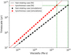 |
Fig. 2 Timescales of orbital circularization for K2-265 b. The red squares (resp. black dots) are the data obtained from the numerical integrations employing the secular code for the initially synchronous (resp. fast-rotating) planet case. The red (resp. black) dashed curves are the corresponding least-square fittings of the results coming from the secular code experiments. The green dashed vertical line on the left (resp. right) is the lower value of the viscosity for which we can reproduce the planet’s current range of eccentricity values for the initially synchronous (resp. fast-rotating) planet case, with τ = τcirc = 6.7 Gyr. |
3.3 The TTVs
In this section, we investigate the TTVs for K2-265 b, where we analyze the influence of tidal interactions as well as other potentially significant effects such as general relativity (henceforth referred to as GR) and stellar rotation. To that end, we employed the Posidonius code, where the creep tide was implemented following the equations presented in the previous section. For the sake of clarity, we separate the analyses into several subsections to discuss the influence of tuning different parameters individually. With the exception of the subsection aimed at discussing the influence of tuning the uniform viscosity coefficient, we considered η = 1022 Pa s in all other simulations. Such a value is consistent with both our orbital circularization timescales and recent estimations of the viscosity in planetary interiors (e.g., silicate mantles with pressure values of P > 25 GPa and the shear to bulk moduli ratio of μ∕K between 0.63 and 0.90 P/K, see Tobie et al. 2019; Bolmont et al. 2020a).
3.3.1 Interplay between apsidal precession and orbital decay
The first aspect to be discussed regarding the TTVs is the relative contribution of orbital decay and apsidal precession. First, we recall the expressions for the transit timings supposing two cases: (i) a circular orbit undergoing orbital decay at rate d a∕dt and (ii) an eccentric orbit undergoing apsidal precession at rate dω∕dt. The expression for the transit timing in the first case reads as follows (see e.g., Ragozzine & Wolf 2009)
![\begin{equation*} t_{\textrm{tra}} (N)\,{=}\,t_0 + NP + \frac{N^2}{2} \left[ \frac{6\pi^2a^2}{G(M+m)}\right] \left(\frac{\textrm{d}a}{\textrm{d}t} \right),\end{equation*}](/articles/aa/full_html/2021/07/aa40202-20/aa40202-20-eq21.png) (16)
(16)
where P is the mean orbital period of the planet.
For the second case, we have, to third-order expansion in the eccentricity (see Giménez & Bastero 1995; Ragozzine & Wolf 2009 for higher-order expansions),
![\begin{eqnarray*} t_{\textrm{tra}} (N)&=& t_0 + NP_{\textrm{S}} + \frac{P_{\textrm{a}}}{\pi} \left[ e \left(\cos \omega _N - \cos \omega _0 \right)\vphantom{\frac{1}{2}} \right.\nonumber\\ && \left.+\,\frac{3}{8} e^2 \left(\sin 2\omega _N - \sin 2\omega _0 \right) + \frac{1}{6} e^3 \left(\cos 3\omega _N - \cos 3\omega _0 \right) \right],\nonumber\\\end{eqnarray*}](/articles/aa/full_html/2021/07/aa40202-20/aa40202-20-eq22.png) (17)
(17)
with t0 and ω0 being the time and argument of the periapsis value of the first reported transit, respectively, and N corresponding to the transit number. Furthermore, the parameters PS and Pa correspond to the sidereal and anomalistic periods, respectively (see e.g., Patra et al. 2017 for more details).
As it can be seen from Eqs. (16) and (17), the contributions coming from apsidal precession and orbital decay to the TTVs have the same dependence on the transit number, that is, both contributions give an N2 dependence on the TTV curves (to first order in cosωN). To disentangle between the effects of apsidal precession and orbital decay on the TTVs, we compared the TTVs obtained by employing two procedures: (i) the data coming from the numerical experiments using the Posidonius code and (ii) synthetic transit curves, which were generated by employing Eqs. (16) and (17). For the synthetic transit curves using Eqs. (16) and (17), we used the values of  and ȧ ensuing from the Posidonius numerical experiment. In the case of a K2-265 b with e = 0.15 and Ω = n, for instance, we have
  and ȧ = −1.91 × 10⁻¹¹ AU yr−1. We would like to mention that in order to investigate the contribution of the apsidal precession to the TTVs, we included the effects of general relativity and stellar rotation in addition to tidal interaction. We verified that the most significant contribution to
  comes from general relativity, which accounts for approximately 93% of the total value of
  . Stellar rotation accounts for approximately 6% of the value of
  (considering the smallest possible rotation period for the star according to Lam et al. 2018 and a stellar k2 of 0.1) and planetary tides account for approximately 1%. Stellar tides play the least important role, contributing less than 1% to
  .
.
Figure 3 shows the results coming from two experiments: one simulation carried out considering only tidal interactions (panel on the left) and one simulation considering general relativity, rotation, and tidal interactions (panel on the right). The contribution of tidally induced orbital decay to the TTVs were filtered out of the orange curve in the right panel of Fig. 3 by directly removing the TTVs generated using Eq. (16). The total integration time was 2 yr, corresponding to approximately 307 transit events for K2-265 b. For the case on the left, we verified that the synthetic curve generated using Eq. (16), which corresponds to the blue curve, gives a TTV amplitude on the order of 0.012 s; whereas, the synthetic curve generated using only Eq. (17), that is to say considering only the contributionof tidally induced apsidal precession to the TTVs, gives a TTV amplitude of approximately 0.0001 s. The negligible role of tidally induced apsidal precession to the TTVs can be verified by comparing the blue solid curve and the orange dashed curve in the left panel. It can be seen that the addition of tidally induced apsidal precession effects on the TTVs does not significantly change the TTV curve, and the orange and blue curves in the left panel are almost identical. However, general relativity plays a non-negligible role in the TTV, with GR-induced apsidal precession being able to produce a TTV amplitude of approximately 20% of the amplitude obtained by considering the tidally induced orbital decay; we recommend for the readers to compare the green curve in the left panel and the orange curve in the right panel in Fig. 3.
Although general relativity has been shown to be non-negligible in the context of the TTVs, its relevance was analyzed for the case of a synchronous planet with η = 1022 Pa s and e = 0.15. It is highly unlikely for a rocky planet with such viscosity and eccentricity values to be in a synchronous rotation rate scenario. Since tidallyinduced orbital decay is bigger for nonsynchronous spin-orbit resonant states, we expect that GR becomes negligible when considering other spin-orbit resonances for the planet. We now analyze how these spin-orbit resonances affect the TTVs.
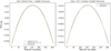 |
Fig. 3 TTVs for K2-265 b, considering η = 1022 Pa s, e = 0.15, and a synchronous rotation rate for the planet. The results on the left were obtained considering only tidal interactions, while the results on the right were obtained by considering tides, rotation, and general relativity (the contribution coming from tidal decay to the TTVs on the orange curve were filtered out by directly subtracting the TTVs generated by employing Eq. (16)). The blue curves in the panels are synthetic TTV curves. The green curve in the left panel and the orange curve in the right panel correspond to the results coming from the Posidonius code. |
3.3.2 The role of eccentricity and planets’ rotation
As it has been discussed in several recent works regarding tidal interactions in rocky bodies, planets with a relatively high viscosity may undergo entrapment in spin-orbit resonances provided that the eccentricity of the planet is bigger than a threshold value and its past rotation was such that Ω ≫ n (e.g., see Correia et al. 2014; Ferraz-Mello 2015 and references therein). Considering the case of the K2-265 b exoplanet with a uniform viscosity of η = 1022 Pa s, several spin-orbit resonant states are stable if we consider the possible eccentricity values for the planet (namely, 0.005 ≤ e ≤ 0.15).
Due to the existence of several stable resonant scenarios, we calculated tidally induced TTVs for the planet for four values of eccentricity, which are within the limit values established by Lam et al. (2018). We also calculated the corresponding spin-orbit stable configurations for each value of eccentricity, where we mention that increasing the eccentricity value leads to the onset of possible higher-order stable spin-orbit resonant states (for details regarding the determination of stable spin-orbit resonances, see e.g., Correia et al. 2014; Ferraz-Mello 2015; Gomes et al. 2019 and references therein). The results of our analysis are shown in Fig. 4. In the figure, we can deduce both the influence of the eccentricity as well as the rotation rate of the planet on the amplitude of the TTVs (henceforth referred to as amp(TTV)), with
 (19)
(19)
By comparing the orange curves in each panel of Fig. 4, it can be seen that the eccentricity value strongly affects the tidally induced TTVs. We verified that amp(TTV) scales with eα, where α = 1, 2 and 4 for the synchronous, 3/2 and 2/1 spin-orbit resonances, respectively. Moreover, α increases monotonically with Ω∕n, the latter usually being referred to as the order of the spin-orbit resonance. At this point, it is worth mentioning that the resulting linear dependence of the amplitude of the TTVs with the eccentricity in the synchronous rotating planet case is consistent with the predictions of Ragozzine & Wolf (2009). We did not perform a study regarding the eccentricity dependence of the amplitudes of the TTVs for higher-order spin-orbit resonances (such as the 5/2 and 3/1 resonances) since such spin-orbit resonances are only maintained at either high eccentricity values with e > 0.15, which are incompatible with the eccentricity estimations of K2-265 b, or very big viscosity values, which are inconsistent with our estimations of Sect. 3.2. Another aspect which can be seen from Fig. 4 by comparing, for instance, the curves in the top left panel is that tidally induced TTVs are negligible for the synchronous rotation and high-order spin-orbit resonant states (e.g., the 5/2 and 3/1 resonances) when compared to the 3/2 and 2/1 resonances (see orange and green curves in each panel).
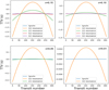 |
Fig. 4 Tidally induced TTV for a timespan of 2 yr (corresponding to 308 transit events), considering several spin-orbit resonances and four values of eccentricity, as indicated in the top right corner of each panel. |
3.3.3 Impact of the uniform viscosity coefficient
Although the combination of eccentricity and age estimations of the system has allowed for a good estimation of the planet’s viscosity, we must analyze the influence of tuning the viscosity value of the planet on the tidally induced TTVs since the viscosity of the planet was estimated with a given uncertainty. For that purpose, we consider viscosity values within the uncertainties discussed in the Sect. 3.2.
Figure 5 shows the TTVs curves for three numerical experiments where we tuned the viscosity value of the planet. We can see that the viscosity is the parameter playing the least important role when compared to the influence of the eccentricity and rotation rate on the amplitudes of the tidally induced TTVs. In Fig. 5, it can be seen that by increasing the viscosity by a factor of 100, the amplitude of the tidally induced TTVs decreases by a factor of approximately 3. The influence of the viscosity value on the TTV amplitude is even weaker for higher-order spin-orbit resonances, as it was verified by some numerical experiments for the 2/1 and 5/2 spin-orbit resonances.
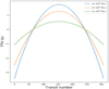 |
Fig. 5 Effect of the viscosity value on the tidally induced TTV for K2-265 b with e = 0.15, Ω∕n = 1.5, and a total transit number of 2 yr. We considered variations of η between theminimum value coming from eccentricity evolution timescale estimations and the maximum value coming from the reference values of Tobie et al. (2019), which were obtained by solving the internal structure equations for the mantle of planets composed by high-pressure silicates. |
3.4 Conditions for potentially observable TTVs
Since we have analyzed the dependency of the tidally induced TTVs with the parameters of the K2-265 system carrying the biggest uncertainties, we can now establish for which conditions we would have the biggest amplitude of tidally induced TTVs (i.e., the scenarios leading to the most easily detectable tidally induced TTVs with the smallest amount of transit data). Figure 6 shows the results concerning such an analysis for the specific case of the 3/2 spin-orbit resonant state, which is the resonant state presenting the biggest TTVs. The curves in the graph give the eccentricity and transit number values leading to the corresponding amplitudes of the TTVs (see labels in the upper right corner of the figure). The dashed brown line corresponds to the maximum value of the eccentricity of K2-265 b estimated by Lam et al. (2018).
From the results shown in Fig. 6, we can conclude that approximately 6 yr (corresponding to approximately 1000 transit events) of transit data would be necessary for a TTV amplitude on the order of 30 s to be obtained, considering that the planet’s eccentricity value is the maximum possible value corresponding to the estimations of Lam et al. (2018). However, if a precision of approximately 10 s for transit measurements is achieved, which is the case for the TRAPPIST-1 system (see discussions in Bolmont et al. 2020b; Agol et al. 2021), we predict that approximately 3.5 yr of transit data would suffice to identify tidally induced TTVs. The follow-up of transit photometry data in the future would then be an essential tool to experimentally identity such effects.
It is worth mentioning that we performed some numerical experiments to evaluate TTVs induced by the stellar tide as well as the stellar flattening resulting from the stellar rotation, where the stellar rotation period of 32.2 days was used in our simulations, following Lam et al. (2018). It was verified that these effects are much smaller than tidally induced TTVs by the planet even in the case of a homogeneous star (i.e., with a fluid Love number of kf = 3∕2). An analysis of the influence of the general relativity on the induced TTVs was also performed. We also verified that these effects are negligible when compared to the planetary tidally induced TTVs.
Although the results presented in this section show that the follow-up of transit data for the K2-265 b could potentially lead to observable TTVs in the near future, we now perform a broad exploration of the tidally induced TTVs as a function of the system’s orbital and physical parameters to have a more comprehensive view of the most important parameters influencing the TTVs.
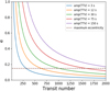 |
Fig. 6 Relation between eccentricity and transit number giving the amplitudes of TTVs indicated in the labels. In all cases, we considered the 3/2 spin-orbit resonance, which gives the highest amplitudes of the TTVs when compared to all the other rotational configurations. The maximum transit number shown in the figure (i.e., 2000 transits) corresponds to approximately 13 yr of transit events. More discussions are presented in the main text. |
4 Broad exploration of the parameters space
In the previous section, we have analyzed tidally induced TTVs for the K2-265 system and concluded that, with the current amount of available data, it is not yet possible to detect tidally induced TTVs. In this section, we explore the influence of other parameters on the values of the tidally induced TTVs with the goal to determine for which exoplanetary systems we would be able to detect such effects with a smaller amount of transit data.
Figure 7 shows the results regarding the exploration of the tidally induced TTVs as a function of four parameters (semi-major axis, planet mass, planet radius, and stellar mass; see labels and caption of Fig. 7). In all panels, the dashed red line corresponds to the case of the K2-265 b planet using the parameters of Table 2. For the bottom panels, we used the normalized transit number to perform the plots since changing the stellar mass and semi-major axis leads to considerable differences in the orbital period, which in turn causes alterations in the total transit number, even though the total time of evolution remains the same (namely, 2 yr). We can clearly see that the most important parameters influencing the amplitudes of the TTVs are the stellar mass and the semi-major axis (see panels c and d in the figure). The planetary radius value also strongly affects the amplitude of the TTVs. However, since super-Earths are believed to have radii between 1 and 1.8 Earth radii, according to recent discussions (see e.g., Fulton et al. 2017), the experiments performed in panel b for Rp = 2 R⊕ and Rp = 3 R⊕ (see orange and green curves) are merely exploratory.
The factor playing the least important role in the TTVs is the planetary mass. Tuning this type of parameter by a factor of 10 leads to a difference in the TTVs of a factor of 3. Moreover, we emphasize that changing the planetary mass leads to a direct change in the relaxation factor value since the planetary mass directly affects the planet mean density value (see Eq. (12)) and its mean equatorial prolateness. Thus, the influence of tuning the planetary mass on the tidally induced TTVs is much more complex than the influences of the other three factors which were considered in this section, and a proportionality relation between the amplitude of the TTVs and the tuning of the planetary mass may not be possible (see orange and green curves in panel a of Fig. 7).
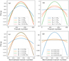 |
Fig. 7 Broad exploration of the TTV as a function of four parameters: (a) planetary mass, (b) planetary radius, (c) stellar mass, and (d) semi-major axis values. We considered a total timespan of 2 yr in all the simulations. In each panel of the figure, we tuned each parameter individually and considered the nominal values of the K2-265 b system for the remaining ones (see Table 2). Moreover, in all cases shown here, we considered a 3/2 spin-orbit resonant state for the planet as well as an eccentricity of 0.15 in order to maximize the effects of the TTVs. |
5 Discussions
In this section, we discuss several aspects of the results obtained in Sects. 3 and 4. For the sake of clarity, the discussions are separated into subsections.
5.1 TTVs for K2-265 b
Regarding our numerical experiments of the TTVs for K2-265 b, we verified that the most important factors ruling the amplitudes of the TTVs are the eccentricity and spin-orbit resonance. Regarding the spin-orbit resonance influence on TTVs, we verified that although synchronous rotation leads to small-amplitude TTVs, planets in low-order spin-orbit resonances (especially the 3/2 and 2/1 resonances) may present relatively high amplitudes of tidally induced TTVs, where the main component causing the tidally induced TTVs for nonsynchronous rotation cases is the orbital decay of the planet. Other effects such as tidally induced apsidal precession and GR-induced apsidal precession were verified to produce TTVs two to three orders of magnitude smaller than the TTVs caused by tidally induced orbital decay. The uniform viscosity coefficient was shown to cause a relatively small variation in the amplitudes of TTVs when compared to the effects of tuning the rotation and eccentricity values.
In what concerns the predictions for future TTVs considering more transit data, we have shown that tidally induced TTVs may be able to cause deviations of transit timings on the order of 30–70 s, considering a 10-yr timespan. These results indicate that tides can be an important source of additional TTVs which are to be included when modeling transit data using a longer baseline in the case of close-in planetary systems.
5.2 Potential confusion with other effects generating TTVs
As it has already been discussed in Sect. 3, the TTVs induced by tidal interactions are much more significant when the planet is trapped in a nonsynchronous spin-orbit resonance, where the main component being responsible for the TTVs is the orbital decay of the planet. However, when the planet is trapped in a synchronous rotation, the TTV induced by orbital decay is less significant, and the TTV induced by the apsidal precession has a non-negligible role in the total TTV. The most significant effect causing apsidal precession-induced TTVs is the GR, with  being at least one order of magnitude bigger than any other effects causing apsidal precession.
Although GR has been shown to play a non-negligible role in the TTVs only in the case of synchronous rotation, it is possible that GR and tides provide the same effects on TTVs if the mass and radius of the planet under study lead to relatively small tidally induced TTVs. In such specific cases, the interplay between GR and tides and their influences on the light curves of exoplanets can be studied by analyzing occultation curves as well as transit curves. As it has been discussed by Patra et al. (2017) and Yee et al. (2020), for example, the shape of the timing variation curves of transits and occultations differ when considering the contributions of apsidal precession and orbital decay. Figure 8 shows an example of occultation timing variation (OTV) curves, corresponding to a homogeneous K2-265 b on a synchronous rotation rate regime with e = 0.15 and η = 1022 Pa s.
Analyzing the contributions coming from orbital decay and apsidal precession to the OTVs shown in Fig. 8, we can see that the occultations provide a way to disentangle between these effects when they have comparable contributions to the timing variations. We emphasize that the use of occultation timing analysis to disentangle between apsidal precession and orbital decay-induced timing variations has already been employed in Yee et al. (2020) to confirm the orbital decay of WASP-12 b, and we briefly present the curves in Fig. 8 to show that tidal interactions and GR can be analyzed separately if occultation data are available (i.e., there is no confusion between the two contributions if both transits and occultation curves are available). However, we emphasize that the only case for which apsidal precession can have a non-negligible effect on the timing curves corresponds to a synchronous rotation, in which case the orbital decay rate is much smaller when compared to nonsynchronous resonant states. In such a specific case, model comparison tools, such as the analysis of the Bayesian information criterion (see discussions in Patra et al. 2017 and Yee et al. 2020), have to be employed to choose between models with different numbers of free parameters (e.g., a model considering a fixed orbital decay rate and a model considering an eccentric orbit with fixed values for the apsidal precession rate and argument of periapsis).
 |
Fig. 8 Occultation timing variations considering the same simulations of Fig. 3, i.e., a K2-265 b with e = 0.15, a synchronous rotation rate, and a viscosity of η = 1022 Pa s. The panel on the left shows the contribution of orbital decay and tidally induced apsidal precession to the OTVs, while the panel on the right shows the contribution of apsidal precession induced by three effects to the OTVs (i.e., for the latter, the effects of GR, tides, and rotation were considered). The synthetic OTV curves were generated by considering Eqs. (5) and (8) given in Sect. 4 of Patra et al. (2017), corresponding to P17 in the labels of the figure. |
5.3 Broad exploration of parameters space
The analysis performed in Sect. 4 regarding the broad exploration of tidally induced TTVs as a function of both planetary and stellar parameters has allowed for the conclusion that the main components leading to significant changes in TTV amplitudes are the stellar mass, planetary radius, and semi-major axis. The planetary mass has been shown to present little influence on the amplitudes of the tidally induced TTVs. Moreover, the results presented in Sect. 4 show that the most promising planetary systems for which tidally induced TTVs would be detectable are the ones for which the orbital period is on the order of 2 days or less, and in which the planet can have a moderate eccentricity on the order of 0.1 or higher, thus allowing for nonsynchronous spin-orbit resonant states to be maintained until the present, thus enhancing the amplitude of tidally induced TTVs when compared to the synchronous rotation rate case.
We emphasize that all calculations presented in this work for the tidally induced TTVs considered that the planet adjusts to hydrostatic equilibrium following a Newtonian creep equation for its shape evolution. We also neglected forced librations of the rotation rate by considering the constant rotation rate approximation of the creep tide theory4. Considering that the planet has permanent components of the flattenings as a consequence of, for example, reorientation or despinning (see e.g., Matsuyama & Nimmo 2008, 2009), this may lead to even bigger TTVs5 . Detecting these permanent shape-induced TTVs may be essential at characterizing planetary interior structures as well as studying their past orbital and rotational configuration.
6 Conclusion
The most important findings of this work regard the analysis of the tidally induced TTVs for nonsynchronous spin-orbit resonant states. For a given eccentricity value, nonsynchronous spin-orbit resonances lead to a faster tidally induced orbital evolution process when compared to synchronous rotation rate cases. As a consequence, planets in nonsynchronous spin-orbit resonances migrate faster and may present larger TTVs than the ones generally predicted by employing classical expressions to calculate the orbital decay rate induced by tides; we refer to classical expressions as the ones generally based on the CTL model, which assumes that the only possible equilibrium rotation state is pseudo-synchronism. Moreover, we have discussed that when occultation timing data are available in addition to transit timing data, the potential degenerescence of tidal interactions with other effects inducing timing variations (such as general relativity and stellar rotation) can be broken by analyzing the occultation timing variations. We also emphasize that in all cases of nonsynchronous rotation, the orbital decay-induced TTV is at least 2 orders of magnitude bigger than the apsidal precession-induced TTV.
Another discussion that ensued from this work is the possibility of the future detection of tidally induced TTVs caused by orbital decay for other exoplanetary systems containing a close-in rocky planet with a non-negligible eccentricity. A quick estimation of the tidally induced TTVs as a function of the semi-major axis in the case of a moderately eccentric planet (with 0.1 < e < 0.2) in the 3/2 spin-orbit resonance allows us to conclude that, for planets with a ≤ 0.02 AU, an amplitude of the tidally induced TTVs on the order of 20−80 s may be reached even for small observation timescales (on the order of 2− 3 yr), provided that the stellar mass is between 0.5 and 1.0 Solar masses. Some of the (putative) single-planet systems in which the planet satisfies such a semi-major axis criterion include, for instance,LHS-3844 b (Vanderspek et al. 2019) and L 168-9 b (Astudillo-Defru et al. 2020). Since very close-in planets are believed to have small eccentricities due to tidally induced orbital circularization processes, the search for the detection of tidally induced TTVs for Earth-like rocky planets may be more advantageous for planetary systems with at least one more planetary companion. In this case, eccentricity excitation as a consequence of planet-planet gravitational interactions could lead to moderate eccentricities for the inner planet. Consequently, nonsynchronous spin-orbit resonances may be maintained until the present. Some of the multiplanet systems which can present this configuration are K2-38 b-c (Sinukoff et al. 2016; Toledo-Padrón et al. 2020), LTT 3780 b-c (Nowak et al. 2020; Cloutier et al. 2020), and TRAPPIST-1 (Gillon et al. 2017). The new version of the Posidonius code introduced in this work, which has been shown to provide stable and precise results, can thus be a powerful tool for studying the cases of these multiplanetary systems, for which analytical formulations of the transit and occultation timings may not be able to capture all the aspects of planet-planet perturbations.
Acknowledgements
The authors would like to thank the anonymous referee for helping improving the manuscript. G.O.G would like to thank FAPESP for funding the project under grants 2016/13750-6, 2017/25224-0 and 2019/21201-0, and David Nesvorný for a fruitful discussion about TTVs. This work has been carried out within the framework of the NCCR PlanetS supported by the Swiss National Science Foundation. This research has made use of NASA’s Astrophysics Data System.
Appendix A Code verification and performance
The Posidonius code considers the effects of additional forces other than N-body point-mass interactions by directly implementing the contribution of these effects in the force components acting on each body of a given system. Both a symplectic integration scheme with a fixed time-step (WHFast integrator) and an integrator with a variable time-step integration scheme (IAS15) are available for use in the code.
To test the proper functioning of the implementation of the creep tide theory in the Posidonius code, we compared the results coming from it with the ones coming from the use of a secular code giving the spin-orbit evolution of the body. The equations for the secular evolution are
![\begin{equation*} \dot{a}\,{=}\,\frac{R^2 n \bar{\epsilon}_{\rho}}{5a} \sum_{k \in \mathbb{Z}} \left[3(2-k) \frac{\gamma (\nu + kn)E_{2,k}^2}{\gamma^2 + (\nu+kn)^2} - \frac{\gamma k^2 n E_{0,k}^2}{\gamma^2 + k^2n^2}\right],\end{equation*}](/articles/aa/full_html/2021/07/aa40202-20/aa40202-20-eq32.png) (A.1)
(A.1)
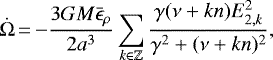
![\begin{equation*} \dot{e}\,{=}\,{-}\frac{3GMR^2 \bar{\epsilon}_{\rho}}{10na^5e} \sum_{k \in \mathbb{Z}} \left[P_k^{(1)} \frac{\gamma (\nu + kn)E_{2,k}^2}{\gamma^2 + (\nu+kn)^2} +\frac{P^{(2)}}{3} \frac{\gamma k^2 n E_{0,k}^2}{\gamma^2 + k^2n^2}\right],\end{equation*}](/articles/aa/full_html/2021/07/aa40202-20/aa40202-20-eq33.png) (A.2)
(A.2)
 (A.3)
(A.3)
where ν = 2Ω − 2n is the semidiurnal frequency of the primary, the coefficients Pk are eccentricity-dependent coefficients given by
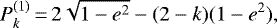 (A.4)
(A.4)
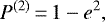 (A.5)
(A.5)
and the coefficients Eq,k are the eccentricity-dependent Cayley coefficients. We can see that no short-period components exist (i.e., components depending on the true or mean anomaly), since they were already averaged out.
Figure A.1 shows an example of the results of three simulations considering the spin and orbit evolution of a homogeneous K2-265 b with a viscosity of η = 1017 Pa s; the choice to consider such a value for η relies on the fact that lower values of η lead to bigger amplitudes of the short-period oscillations of Ω, thus representing the best scenario for identifying potential changes introduced by the averaging of the equations of motion, which are performed in the frame of the secular model.
We can see several characteristics which are classic of tidal evolution scenarios in Fig. A.1: firstly, the rotation of the planet is damped to a 2/1 spin-orbit resonant state. This process is followed by orbital shrinking and eccentricity damping until the 2/1 spin-orbit resonance is no longer stable. The rotation then evolves to the 3/2 spin-orbit resonance while the eccentricity and semi-major axis continue to decrease; we emphasize that the evolution of the orbit takes place on a timescale that is much bigger than the evolution of the rotation. The endpoint of tidal evolution is achieved when both orbital circularization and rotational synchronization take place. We can see that the values of the orbital elements at the endpoint of the tidal evolution are in very good agreement with the analytical estimations coming from the angular momentum conservation of the system, namely  (see red dashed curve in the top panel on the left in Fig. A.1).
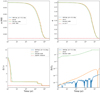 |
Fig. A.1 Semi-major axis, eccentricity, rotation, and angular momentum evolution of four simulations (see the labels in the panels). Solid lines correspond to simulations using the Posidonius code, and the green dashed line corresponds to the simulation using the secular code. The red dashed line shown in the panels of the orbital and rotational evolution of the planet corresponds to the predictions of the final values of the spin-orbit configuration of the planet, based on total angular momentum conservation. |
From the point of view of angular momentum conservation, we can see that the Posidonius code conserves it with a much better precision when compared to the secular code (see bottom panel on the right in Fig. A.1). Additionally, we verified thatthe WHFast code better conserves the angular momentum for a sufficiently long timescale, whereas the IAS15 integrator gives more precise results for short-term evolution scenarios. Lastly, we comment that the speed of integration is much slower for the IAS15 when compared to the WHFast integrator. The ratio of time taken to evolve the orbits with the IAS15 and WHFast integrators is approximately 25, which is an expected difference inintegration time given the adaptative time-step scheme of the IAS15 integrator. We note that the value of the constant time-step chosen for the WHFAST was set so that it would be near the mean value of the time-step chosen by the adaptative time-step algorithm of the IAS15 integrator (for the latter case, we verified that the time-step oscillated between 0.08 and 0.13 days for the simulation shown in Fig. A.1). We also performed some experiments by tuning the time-step of the WHFast integrator and verified that the results obtained by considering a time-step smaller than 0.1 days do not change when compared to the case in which the time-step was chosen to be 0.1 days (i.e., the case corresponding to the blue curve in Fig. A.1). For a more comprehensive discussion on the precision and error analyses for symplectic integrators, see Hernandez & Dehnen (2017).
References
- Agol, E., Steffen, J., Sari, R., & Clarkson, W. 2005, MNRAS, 359, 567 [Google Scholar]
- Agol, E., Dorn, C., Grimm, S. L., et al. 2021, Planet. Sci. J., 2, 1 [Google Scholar]
- Astudillo-Defru, N., Cloutier, R., Wang, S. X., et al. 2020, A&A, 636, A58 [CrossRef] [EDP Sciences] [Google Scholar]
- Ballard, S., Chaplin, W. J., Charbonneau, D., et al. 2014, ApJ, 790, 12 [NASA ADS] [CrossRef] [Google Scholar]
- Blanco-Cuaresma, S., & Bolmont, E. 2017, in EWASS Special Session 4 (2017): Star-planet interactions (EWASS-SS4-2017) [Google Scholar]
- Bolmont, E., Breton, S. N., Tobie, G., et al. 2020a, A&A, 644, A165 [CrossRef] [EDP Sciences] [Google Scholar]
- Bolmont, E., Demory, B. O., Blanco-Cuaresma, S., et al. 2020b, A&A, 635, A117 [EDP Sciences] [Google Scholar]
- Cloutier, R., Eastman, J. D., Rodriguez, J. E., et al. 2020, AJ, 160, 3 [Google Scholar]
- Correia, A. C. M., & Delisle, J.-B. 2019, A&A, 630, A102 [CrossRef] [EDP Sciences] [Google Scholar]
- Correia, A. C. M., Boué, G., Laskar, J., & Rodríguez, A. 2014, A&A, 571, A50 [NASA ADS] [CrossRef] [EDP Sciences] [Google Scholar]
- Delisle, J. B., Correia, A. C. M., Leleu, A., & Robutel, P. 2017, A&A, 605, A37 [NASA ADS] [CrossRef] [EDP Sciences] [Google Scholar]
- Efroimsky, M. 2012, ApJ, 746, 150 [Google Scholar]
- Efroimsky, M. 2018, Icarus, 306, 328 [Google Scholar]
- Ferraz-Mello, S. 2013, Celest. Mech. Dyn. Astron., 116, 109 [Google Scholar]
- Ferraz-Mello, S. 2015, Celest. Mech. Dyn. Astron., 122, 359 [Google Scholar]
- Folonier, H. A., Ferraz-Mello, S., & Andrade-Ines, E. 2018, Celest. Mech. Dyn. Astron., 130, 78 [Google Scholar]
- Fressin, F., Torres, G., Charbonneau, D., et al. 2013, ApJ, 766, 81 [NASA ADS] [CrossRef] [Google Scholar]
- Fulton, B. J., Petigura, E. A., Howard, A. W., et al. 2017, AJ, 154, 109 [Google Scholar]
- Gillon, M., Triaud, A. H. M. J., Demory, B.-O., et al. 2017, Nature, 542, 456 [Google Scholar]
- Giménez, A.,& Bastero, M. 1995, Ap&SS, 226, 99 [Google Scholar]
- Gomes, G. O., Folonier, H. A., & Ferraz-Mello, S. 2019, Celest. Mech. Dyn. Astron., 131, 56 [Google Scholar]
- Haswell, C. A. 2018, WASP-12b: A Mass-Losing Extremely Hot Jupiter, eds. H. J. Deeg, & J. A. Belmonte (Berlin: Springer), 97 [Google Scholar]
- Hebb, L., Collier-Cameron, A., Loeillet, B., et al. 2009, ApJ, 693, 1920 [Google Scholar]
- Hernandez, D. M., & Dehnen, W. 2017, MNRAS, 468, 2614 [Google Scholar]
- Lam, K. W. F., Santerne, A., Sousa, S. G., et al. 2018, A&A, 620, A77 [NASA ADS] [CrossRef] [EDP Sciences] [Google Scholar]
- Lithwick, Y., Xie, J., & Wu, Y. 2012, ApJ, 761, 122 [Google Scholar]
- Love, A. E. H. 1911, Some Problems of Geodynamics (Cambridge: Cambridge University Press) [Google Scholar]
- Makarov, V. V., & Efroimsky, M. 2013, ApJ, 764, 27 [Google Scholar]
- Matsuyama, I., & Nimmo, F. 2008, Icarus, 195, 459 [Google Scholar]
- Matsuyama, I., & Nimmo, F. 2009, J. Geophys. Res. Planets, 114, E01010 [Google Scholar]
- Mayor, M., Pepe, F., Queloz, D., et al. 2003, The Messenger, 114, 20 [NASA ADS] [Google Scholar]
- Mignard, F. 1979, Moon and Planets, 20, 301 [Google Scholar]
- Nesvorný, D., & Morbidelli, A. 2008, ApJ, 688, 636 [Google Scholar]
- Nesvorný, D., & Vokrouhlický, D. 2016, ApJ, 823, 72 [Google Scholar]
- Nowak, G., Luque, R., Parviainen, H., et al. 2020, A&A, 642, A173 [NASA ADS] [CrossRef] [EDP Sciences] [Google Scholar]
- Patra, K. C., Winn, J. N., Holman, M. J., et al. 2017, AJ, 154, 4 [Google Scholar]
- Pedregosa, F., Varoquaux, G., Gramfort, A., et al. 2011, J. Mach. Learn. Res., 12, 2825 [Google Scholar]
- Ragozzine, D., & Wolf, A. S. 2009, ApJ, 698, 1778 [Google Scholar]
- Rein, H., & Spiegel, D. S. 2015, MNRAS, 446, 1424 [NASA ADS] [CrossRef] [Google Scholar]
- Rein, H., & Tamayo, D. 2015, MNRAS, 452, 376 [Google Scholar]
- Rodríguez, A., Callegari, N., & Correia, A. C. M. 2016, MNRAS, 463, 3249 [Google Scholar]
- Sinukoff, E., Howard, A. W., Petigura, E. A., et al. 2016, ApJ, 827, 78 [Google Scholar]
- Sullivan, P. W., Winn, J. N., Berta-Thompson, Z. K., et al. 2015, ApJ, 809, 77 [NASA ADS] [CrossRef] [Google Scholar]
- Tobie, G., Grasset, O., Dumoulin, C., & Mocquet, A. 2019, A&A, 630, A70 [CrossRef] [EDP Sciences] [Google Scholar]
- Toledo-Padrón, B., Lovis, C., Suárez Mascareño, A., et al. 2020, A&A, 641, A92 [CrossRef] [EDP Sciences] [Google Scholar]
- Vanderspek, R., Huang, C. X., Vanderburg, A., et al. 2019, ApJ, 871, L24 [NASA ADS] [CrossRef] [Google Scholar]
- Walterová, M., & Běhounková, M. 2020, ApJ, 900, 24 [Google Scholar]
- Yee, S. W., Winn, J. N., Knutson, H. A., et al. 2020, ApJ, 888, L5 [Google Scholar]
- Youdin, A. N. 2011, ApJ, 742, 38 [Google Scholar]
We emphasize that a self-consistent formulation for the coupled spin-orbit and shape evolution considering a Maxwell rheology for the planet was presented in Correia et al. (2014), which was extended to study (i) three-body exoplanetary systems by Rodríguez et al. (2016) and Delisle et al. (2017) and (ii) N-body systems by Correia & Delisle (2019).
The new version of the code including the implementation of the creep tide theory is available for download in https://github.com/gabogomes/posidonius/tree/posidonius-creep, and the original Posidonius website is https://www.blancocuaresma.com/s/posidonius
We note that the expansion in eccentricity coefficients presented in this work converges only for eccentricities up to ≈0.40. For a formulation of the creep tide theory allowing arbitrary eccentricity values, see Folonier et al. (2018).
For planets trapped in spin-orbit resonances, forced librations can have an important role on the tidal heating of the planets (see e.g., discussions in Efroimsky 2018; Correia & Delisle 2019).
To take permanent components of the flattenings into account, a different implementation of tidal interactions must be used. In the frame of the creep tide, for instance, we would have to solve three additional first-order differential equations, dictating the shape evolution of the body instead of supposing the constant rotation rate approximation, which automatically neglects forced librations of the rotation rate (see e.g., discussions in Folonier et al. 2018; Gomes et al. 2019).
All Tables
Physical and orbital parameters for K2-265 b and its host star after Lam et al. (2018).
All Figures
|
Fig. 1 Scheme of the geometrical setup considered in the framework of the creep tide theory, partially reproduced from Folonier et al. (2018). On the left, we have the pure static case in which the primary always points toward the companion, which is at a distance r from the primary. On the right, we have the case in which the response of the primary is delayed due to the primary’s nonzero viscosity value. In both panels,
|
| In the text | |
|
Fig. 2 Timescales of orbital circularization for K2-265 b. The red squares (resp. black dots) are the data obtained from the numerical integrations employing the secular code for the initially synchronous (resp. fast-rotating) planet case. The red (resp. black) dashed curves are the corresponding least-square fittings of the results coming from the secular code experiments. The green dashed vertical line on the left (resp. right) is the lower value of the viscosity for which we can reproduce the planet’s current range of eccentricity values for the initially synchronous (resp. fast-rotating) planet case, with τ = τcirc = 6.7 Gyr. |
| In the text | |
|
Fig. 3 TTVs for K2-265 b, considering η = 1022 Pa s, e = 0.15, and a synchronous rotation rate for the planet. The results on the left were obtained considering only tidal interactions, while the results on the right were obtained by considering tides, rotation, and general relativity (the contribution coming from tidal decay to the TTVs on the orange curve were filtered out by directly subtracting the TTVs generated by employing Eq. (16)). The blue curves in the panels are synthetic TTV curves. The green curve in the left panel and the orange curve in the right panel correspond to the results coming from the Posidonius code. |
| In the text | |
|
Fig. 4 Tidally induced TTV for a timespan of 2 yr (corresponding to 308 transit events), considering several spin-orbit resonances and four values of eccentricity, as indicated in the top right corner of each panel. |
| In the text | |
|
Fig. 5 Effect of the viscosity value on the tidally induced TTV for K2-265 b with e = 0.15, Ω∕n = 1.5, and a total transit number of 2 yr. We considered variations of η between theminimum value coming from eccentricity evolution timescale estimations and the maximum value coming from the reference values of Tobie et al. (2019), which were obtained by solving the internal structure equations for the mantle of planets composed by high-pressure silicates. |
| In the text | |
|
Fig. 6 Relation between eccentricity and transit number giving the amplitudes of TTVs indicated in the labels. In all cases, we considered the 3/2 spin-orbit resonance, which gives the highest amplitudes of the TTVs when compared to all the other rotational configurations. The maximum transit number shown in the figure (i.e., 2000 transits) corresponds to approximately 13 yr of transit events. More discussions are presented in the main text. |
| In the text | |
|
Fig. 7 Broad exploration of the TTV as a function of four parameters: (a) planetary mass, (b) planetary radius, (c) stellar mass, and (d) semi-major axis values. We considered a total timespan of 2 yr in all the simulations. In each panel of the figure, we tuned each parameter individually and considered the nominal values of the K2-265 b system for the remaining ones (see Table 2). Moreover, in all cases shown here, we considered a 3/2 spin-orbit resonant state for the planet as well as an eccentricity of 0.15 in order to maximize the effects of the TTVs. |
| In the text | |
|
Fig. 8 Occultation timing variations considering the same simulations of Fig. 3, i.e., a K2-265 b with e = 0.15, a synchronous rotation rate, and a viscosity of η = 1022 Pa s. The panel on the left shows the contribution of orbital decay and tidally induced apsidal precession to the OTVs, while the panel on the right shows the contribution of apsidal precession induced by three effects to the OTVs (i.e., for the latter, the effects of GR, tides, and rotation were considered). The synthetic OTV curves were generated by considering Eqs. (5) and (8) given in Sect. 4 of Patra et al. (2017), corresponding to P17 in the labels of the figure. |
| In the text | |
|
Fig. A.1 Semi-major axis, eccentricity, rotation, and angular momentum evolution of four simulations (see the labels in the panels). Solid lines correspond to simulations using the Posidonius code, and the green dashed line corresponds to the simulation using the secular code. The red dashed line shown in the panels of the orbital and rotational evolution of the planet corresponds to the predictions of the final values of the spin-orbit configuration of the planet, based on total angular momentum conservation. |
| In the text | |
Current usage metrics show cumulative count of Article Views (full-text article views including HTML views, PDF and ePub downloads, according to the available data) and Abstracts Views on Vision4Press platform.
Data correspond to usage on the plateform after 2015. The current usage metrics is available 48-96 hours after online publication and is updated daily on week days.
Initial download of the metrics may take a while.