| Issue |
A&A
Volume 649, May 2021
|
|
|---|---|---|
| Article Number | A48 | |
| Number of page(s) | 24 | |
| Section | Galactic structure, stellar clusters and populations | |
| DOI | https://doi.org/10.1051/0004-6361/202040017 | |
| Published online | 10 May 2021 | |
Orbital eccentricities as indicators of stellar populations
A kinematical analysis of the local disc from Gaia DR2 catalogue
1
Dept. Matemàtica Aplicada, Universitat Politècnica de Catalunya, 08034 Barcelona, Catalonia, Spain
e-mail: This email address is being protected from spambots. You need JavaScript enabled to view it.
2
Astronomical Observatory, Volgina 7, 11060 Beograd 38, Serbia
e-mail: This email address is being protected from spambots. You need JavaScript enabled to view it.
3
Institute Isaac Newton of Chile, Yugoslavia Branch, Serbia
Received:
30
November
2020
Accepted:
29
January
2021
Abstract
Aims. Based on a local sample from Gaia DR2 catalogue composed of 74 339 stars, we are able to derive more accurate kinematic statistics defining the local stellar populations and classify the stars in terms of their planar and vertical orbital eccentricities.
Methods. Firstly, we carried out a kinematical characterisation of stellar populations from a tested mixture model that fits the trivariate velocity cumulants up to the fourth order, maximises the entropy of the mixture probability, and minimises the χ2 error. We then proposed several approaches to classifying the stars according to the population they are most likely to belong to. None of these approaches provided a definitive solution due to the overlapping of the partial distributions. Finally, by using the epicycle approximation, we transformed the three-dimensional velocity probability space into a two-dimensional diagram. In one direction, the information of the two planar velocity components is picked up by the planar eccentricity. In the other direction, the vertical eccentricity does the same with the vertical velocity component. However, in the vertical direction, the epicycle approximation is not valid and it is replaced by a biquadratic approximation.
Results. In the eccentricity diagram, the region of maximum probability for a population is approximately delimited by straight line. We characterise three local kinematic populations: thin disc, thick disc (composed of two subpopulations: canonical thick disc and metal-weak thick disc), and kinematical halo (metal-rich thick-disc plus chemical halo). The Gaia DR2 sample allows us to estimate small mean radial differential motion of 5 ± 2 km s−1 between the thin and thick discs, and of 9 ± 3 km s−1 between both thick-disc subpopulations, as well as between the disc and the kinematical halo. All disc populations and subpopulations have significant vertex deviations.
Conclusions. The classification of the stars from the eccentricity diagram resolves the problem of overlapping velocity distributions by producing a segregation that is more net, along with a more precise kinematical characterisation of populations.
Key words: Galaxy: kinematics and dynamics / Galaxy: disk / stars: kinematics and dynamics / stars: Population II
© ESO 2021
1. Introduction
In recent years, the statistical analysis of local kinematic populations was drastically limited by the amount of data available, mainly with regard to radial velocities. The advent of the HIPPARCOS Catalogue (ESA 1997) represented both a qualitative and quantitative change for the better. Previously, a typical local disc sample limited to a trigonometric distance of 300 pc consisted of 13 678 stars (e.g., Cubarsi & Alcobé 2004; Alcobé & Cubarsi 2005). To understand the extent of such an improvement, it suffices to compare the size, N, of such a sample with the one used by Erickson (1975) to compute, for the first time, the higher-order central velocity moments, composed of 869 stars. In addition, we must recall that the sampling variances of the moments are proportional to  .
.
The Geneva-Copenhagen survey (GCS) catalogue (Nordström et al. 2004; Holmberg et al. 2007) incorporated new and more accurate radial velocity data. However, a sample composed of F and G dwarf stars, considered the favourite tracer populations of the history of the disc, contained the total velocity space of 13 240 stars. Hence, this sample improved the quality of the data, but not the size. The GCS catalogue allowed for some previous results to be confirmed while improving others (Famaey et al. 2007; Cubarsi et al. 2010); in particular, the detail of the small-scale of the local velocity distribution (Skuljan et al. 1999; Dehnen & Binney 1998; Soubiran & Girard 2005; Famaey et al. 2005), which was proven to be strongly correlated with the planar eccentricity of the stars’ orbits (Cubarsi 2010).
By using newer radial velocity data from the RAdial Velocity Experiment (RAVE) survey (Siebert et al. 2011; Zwitter et al. 2008; Steinmetz et al. 2006), which incorporated the radial velocity of 49 327 randomly selected stars, several statistical analyses (Pasetto et al. 2012a,b; Steinmetz 2012; Moni Bidin et al. 2012; Casetti-Dinescu et al. 2011; Smith et al. 2009a,b) have studied the velocity distribution of the galactic populations from neighbourhood stellar samples of about 39 000 stars. Thanks to this more accurate data, it was possible to estimate the anisotropy of the velocity distribution and to assert that thick disc stars have a radial mean motion that differs from the thin disc. In addition, inside the thick disc, a subdivision was proposed between a rapidly rotating canonical thick disc and a metal-weak thick disc (MWTD). Inside the halo, the outer and counter-rotating halo was differentiated from the inner halo (Carollo et al. 2010, 2019; Kordopatis et al. 2013; Beers et al. 2014). However, we might consider whether such sets of stars should be considered as independent populations (Haywood et al. 2018), since Di Matteo et al. (2019) proved that the kinematically defined halo in the solar neighbourhood is approximately composed of a half of metal-rich thick-disc (MRHD) stars and a half of chemical halo stars.
More recently, the European Space Agency’s Gaia mission (Gaia Collaboration 2016) produced Gaia’s second data release (Gaia DR2, Gaia Collaboration 2018) and just a few weeks ago, Gaia EDR3 (Gaia Collaboration 2021a) was released. Gaia DR2 provides position, parallax, and proper motions for ca. 1.3 × 10⁹ stars in the Milky Way (Lindegren et al. 2018) and radial velocity for about 7.2 million stars (Soubiran et al. 2018) measured using a Radial Velocity Spectrograph (Cropper et al. 2018). With regard to the stellar density distribution, the precise measurement of the parallax for the bright stars allows to focus in selected populations of stars (Miyachi et al. 2019; Galli et al. 2019). With regard to the velocity distribution, Gaia radial velocities have an even better precision than those of RAVE (Sysoliatina et al. 2018; Katz et al. 2019), and the radial velocities catalogue is more complete, with a simpler completeness function, and reproduces the vertical kinematics of the disc.
In this work, we use a local sample of Gaia DR2, composed of 74 339 stars within a solar radius of 100 pc, to characterise in a more precise way the kinematic statistics used to define the local stellar populations. From the statistical analysis of the velocity space, we wish to infer some key values for the orbital eccentricities, allowing for a net separation of the local galactic populations.
2. Preliminaries
2.1. Stellar populations
The concept of stellar population can carry various implications. For instance, it can refer to the chemical composition of the stars or, alternatively, it can describe their main kinematic features through their mean velocity and the associated tensor of covariances. In this paper, we focus on the kinematical approach.
From the kinematical viewpoint, a stellar population is typically composed of many subsets of stars, possibly with well-defined properties for each subset, such as it happens with moving groups or stellar streams composing the galactic disc. But a moving group itself is not a statistical population. As described in Cubarsi (2010), the small-scale kinematics of the disc is determined by stellar streams that are associated with stars of low planar eccentricity. When stars with greater eccentricities are considered, the specific kinematic behaviour of the stellar streams is no longer seen and an average behaviour of the whole set dominates.
From a statistical viewpoint, according to the law of large numbers, the sample average of the stars that have velocities with similar distribution tends to a Gaussian distribution that characterises the kinematics of the statistical population. In other words, a sufficiently large number of stars is required for it to be possible to speak of a continuous velocity distribution that describes, in terms of its mean values and moments (similarly to the kinetic theory of gases) the macroscopic state of a population as a whole. To this, the condition of statistical equilibrium must be added, meaning that the phase space density function of each population, which depends the particular integrals of motion of its stars, is invariant under the collisionless Boltzmann equation. Such a condition is satisfied when each population is of a Schwarzschild type (e.g., Chandrasekhar 1942; Ogorodnikov 1965; Lynden-Bell 1967), meaning that there is a Gaussian distribution in the three-dimensional velocity space, which is a particular case of ellipsoidal distribution. Moreover, since this equation is linear, we may assume (Cubarsi 2018) that the whole stellar system is composed of a finite number of stellar populations in statistical equilibrium.
Ellipsoidal distributions are described in terms of their central second moments (tensor of covariances) μ2, which can be written in terms of the peculiar velocity components as (e.g., Binney & Tremaine 2008):
The second central moments account for the shape and orientation of the velocity ellipsoid and for the variance  of the velocity distribution function in an arbitrary direction, l, of the peculiar velocity space. According to the coordinate system, if c1, c2, and c3 are the corresponding direction cosines, we have:

The symmetric tensor  (inverse of the second central moments μ2) is then associated with the peculiar velocity ellipsoid:
so that the velocity dispersions σ1, σ2, and σ3 are the semiaxes of the ellipsoid that refers to the same coordinate axes. The anisotropy of the velocity ellipsoid is measured by the ratio of the velocity dispersions along the principal axes and by its orientation since the principal axes need not to be aligned with the coordinate axes. The angle between the direction from the Sun to the Galactic Centre (GC) and the direction of the major principal axis of the velocity ellipsoid is known as vertex deviation, while the angle between the major principal axis and the Galactic Plane (GP) is the tilt of the velocity ellipsoid.
In general, and especially when the velocity variables are expressed without subindices, the nth central moments can be written as (e.g., Gilmore et al. 1990):
 (1)
(1)
with α + β + γ = n. This notation is used in the current paper.
In the current paper, a stellar group is referred to as a stellar population if it can be reasonably approximated by a trivariate Gaussian distribution, otherwise we refer to subpopulation. Such a simplified Galaxy model with a few population components is useful for getting a large-scale kinematical portrait depicting the basic symmetries of the stellar velocity distribution – or the main deviations from them (Cubarsi 2014a,b) – such as whether there is axial or point-axial symmetry and a symmetry plane, what the average differential motion between populations is, as well as the shape and orientation of the respective velocity ellipsoids, etc. In addition, these features are relative to the potential function of the dynamical model.
2.2. Orbital eccentricities
As stated above, the velocity distribution function depends on the isolating integrals of the star motion. The disc and the halo stars may share some integrals of motion, for example, the energy integral, I1, (under the hypothesis of steady-state system) and the angular momentum integral, I2, (under the hypothesis of axial symmetry). Nevertheless, for disc stars, an independent integral, I3, (e.g., Gilmore et al. 1990), related to the low height about the GP allowing for the approximation of separability of the potential in cylindrical coordinates, makes them distinguishable from halo stars. Hence, a combination of these integrals defines a quadratic form, Q, that is, the velocity ellipsoid, which characterises the Schwarzschild velocity distribution that defines the stellar population based on its means and second central moments.
For a population mixture, the velocity moments of the whole stellar sample allow us to determine, with an acceptable accuracy, the population partial moments (Cubarsi et al. 2010). However, in the process of disentangling the partial distributions, the stars belonging to a region where the tails of the population distributions overlap then become classified with a great level of uncertainty. Other non-kinematical parameters can be of help, such as the metallicity [Fe/H] and the colour b − y, but none of them produce a net segregation (Cubarsi 2010). The alternative approach presented here, still based on kinematical parameters, is meant to identify the thin and thick disc stars from its planar and vertical eccentricities. In this way, the problem of such overlapping regions is to become minimised. The reason is that for the disc stars, the equations of the star motion can be treated as two independent sets: one for the planar motion in the GP, involving the integrals I1 − I3 and I2, which are in direct relation to the planar eccentricity of the star (Ninković 2018), and another, for the perpendicular motion, involving the integral I3, which is in direct relation to the vertical eccentricity.
Let us recall the definitions of planar and vertical eccentricities. For a local disc star, under the epicycle approximation (e.g., Binney & Tremaine 2008), the local radius r0 and the radius rc of the circular velocity point C1 can be expressed in terms of the maximum and minimum orbital distances to the centre, ra and rp (apo- and pericentric distances), as  . Then, the planar eccentricity is defined from the orbital amplitude a, as:
 (2)
(2)
On the other hand, the vertical eccentricity, e′, is defined in terms of the maximum height, zmax, about the GP as:
 (3)
(3)
The approach based on the epicycle approximation was proven to be a promising tool in Cubarsi et al. (2010) when working with the Geneva-Copenhagen Survey III catalogue (Holmberg et al. 2009); in Cubarsi et al. (2017), it allowed the authors of the study to infer features of the local potential in relation to several symmetry hypotheses.
2.3. Stellar sample
We used two criteria to obtain our local sample. Firstly, we selected all the stars that have parallax greater than 10 mas. Then, from these sources, we selected those that satisfy the two following conditions: the astrometric parameters are solved and for ever source, the radial velocities must be given. In this way, we obtained a sample consisting of 74 339 stars.
Sources with poor astrometric solutions are expected to have small parallaxes, so they should not present a potential contamination of our sample. As for radial velocities, in Gaia DR2, there are about 4000 stars that have been reported to carry erroneous values (information available on the site2) and for this reason, they are not present in Gaia EDR3, pending further tests of the local kinematics, however, we decided to keep them based on the presumption that those stars most likely belong to the halo. Halo stars are known to be rare, but our interest is to have as many of them as possible in our sample.
Our examination shows that if Gaia EDR3 were used, our sample would be slightly smaller. As for five-parameter astrometry solution, in Gaia EDR3, only the errors are different. For instance, Gaia Collaboration (2021b), in applying a quite different approach, have found 74 281 stars within 100 pc from the Sun with radial velocities, a conclusion that is rather similar to our own.
When our sample of stars was finally constructed, we looked further into the Gaia DR2 catalogue to analyse the metallicities given by the Gaia team. Since we used only the sources with measured radial velocity, all these sources also have values for [Fe/H] that are given from the template parameters (Katz et al. 2019). The metallicities given in the catalogue may serve as indicators because it is well-known that thin-disc stars are generally the most metal-rich, whereas halo stars tend to be generally the most metal-poor.
In order to determine the planar eccentricity and the maximum height of the Galactocentric orbits, we used the model of the Milky Way proposed by Ninković (1992). This model assumes three contributors to the potential of the Milky Way: the bulge, the disc, and the corona (the subsystem consisting of dark matter). The latter is assumed as spherically symmetric, while the other ones are assumed to be axisymmetric. The contributions to the Galactic potential of the former two are described by the same formula as that of Miyamoto & Nagai (1975). The only difference concerns the values of the parameters. The parameters from Gaia DR2 (five-parameter astrometry solution and radial velocity) are used as input for the model. The integration of the Galactocentric orbits for each star is done for 10 Gyr by using a fourth-order Runge-Kuta method, from where we obtained values for ra, rp, and zmax.
2.4. Methods
Our procedure consists of three steps. Firstly, we made a kinematical characterisation of the stellar components (further described in Sect. 3) by applying the same statistical algorithm (Cubarsi et al. 2010, hereafter Paper I) used for other catalogues. The algorithm (a) uses a mixture model that fits the trivariate cumulants up to the fourth order, (b) maximises the entropy of the mixture probability according to a hierarchical segregation, and (c) minimises the χ2 error of the total set of cumulants, which, in the optimal case, matches the maximum entropy condition. In this way, it is possible to determine the sampling parameters by allowing subsamples to be extracted, which contain either a mixture of thin and thick discs, or a mixture of disc and halo. As a result, each population remains characterised by its mean velocity, its covariance matrix, and the mixture proportion. For the disc, the most reliable samples are those obtained when the sampling parameter is the absolute heliocentric velocity (the improvement achieved when using the peculiar velocity is not significant and requires a more laborious iterative process). We are able to confirm that there is vertex deviation in the thin and thick discs, although their differential radial motion is very small. In addition, the MWTD, together with a part of the MRHD stars, are still identified as belonging to the same extreme subpopulation of the disc. Alternatively, when the samples are selected from the absolute perpendicular velocity, it is possible to discriminate between the thick disc and the kinematical halo composed of MRHD stars and a few chemical halo stars.
In a second step (described in Sect. 4), the stars are labelled according to the population they most likely belong to. Three plausible criteria are applied and discussed, each having their pros and cons, and ultimately, none of them provide a definitive solution for identifying a star from its velocity components when these components belong to an overlapping region with similar population probability. Thus, after the stars have been labelled as belonging to one of the populations, we may extract subsamples of supposedly pure populations, although none of these subsamples will have bell-shaped distribution, typical of the Gaussian distributions, in any of the velocity variables.
In a third step (Sect. 5), the most likely population is obtained, not in terms of the velocities, but in terms of the eccentricities. By using the epicycle approximation for the disc stars, we transform the three-dimensional velocity probability space into a two-dimensional diagram. In one direction, the information of the two planar velocity components is picked up by the planar eccentricity, e. In the other direction, the vertical eccentricity, e′, does the same with the vertical velocity component. Nevertheless, upon moving away from the GP, the epicycle approximation is no longer valid and requires an approximate model, which is fitted by using a biquadratic equation for the vertical velocity curve. In the eccentricity diagram (e′2 in terms of e2), three regions of maximum likelihood with regard to the populations become delimited by two nearly straight lines. When the classification of the stars is carried out according to these regions, the resulting subsamples recover the bell-shaped curve in each velocity component, their covariances match those expected for the corresponding populations and are obtained with smaller sampling variances. Additionally, it solves the overlapping problem of the distributions by producing a more net segregation.
3. Populations in the sample
3.1. Segregation algorithm
The method to identify kinematic populations is explained with detail in Paper I. It was referred to as MEMPHIS algorithm. Briefly, it consists of several complementary criteria.
We use a continuous sampling parameter P allowing to form nested stellar subsamples that incorporate subsequent populations orderly. There are two optimal sampling parameters, namely P = |v|, the absolute value of the heliocentric star velocity3v = (U, V, W), and P = |W|.
The algorithm segregates pairs of Gaussian populations (1 and 2). For consecutive segregations, population 1 is cumulative (i.e. it approximates the previous segregated populations by a single Gaussian component). As they increase the sampling parameter, subsequent entering populations are identified as population 2.
There are two indicators for validating the goodness of a segregation. One is the entropy of the partition H, which must attain a relative maximum at the end of a region of stability. The other is the χ2 error, associated with the fitting of the velocity cumulants up to the fourth order, which must reach a relative minimum. For optimal cases, such extreme values are achieved simultaneously.
3.2. Selecting by P = |v|
3.2.1. Inside the thin disc
The sampling parameter P = |v| yields an optimal segregation for P = 50 km s−1, as it is shown in Fig. 1. However, the large χ2 error with regard to the subsequent optimal points is indicative of the poor Gaussianity of both segregated components. This result is similar to that obtained in Alcobé & Cubarsi (2005) for HIPPARCOS samples, which was interpreted as a mixture of early-type stars and young disc stars, whose most important differential movement took place in the radial direction. According to Cubarsi (2010), such a subsample reflects the kinematics of the Hyades-Pleiades moving groups and the Sirius-UMa stream, and is not yet kinematically representative of the whole thin disc.
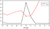 |
Fig. 1. Local optimal values of the partition entropy, H (dimensionless), and χ2 (scaled error) obtained from the sampling parameter P = |v| inside the thin disc. |
3.2.2. Thin and thick discs
The optimal values are shown in Fig. 2. The values P = 123 and P = 230 km s−1 detect a mixture of thin and thick disc populations. The former identifies the core of the thin disc, t, as population 1, and a partial thick disc4, the canonical thick disc T−, as population 2. On the other hand, the sample selected by P = 230, also contains a new subpopulation, the MWTD stars, say T+. From a kinematical viewpoint, there are two subpopulations within the thick disc, which altogether but not separately, can be approximated by a Gaussian distribution. The velocity moments (centred and non-centred) of the selected stellar subsamples are listed in the Appendix D, and the partial centred moments of the population components in Table 1. The notation used here is that of Eq. (1).
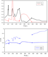 |
Fig. 2. Optimal values from the sampling parameter P = |v| (km s−1). Top: entropy, H (dimensionless), and χ2 (scaled error). Bottom: trend of the radial velocity dispersion σ1 (on a logarithmic scale). |
Mean velocities (km s−1), second central moments (km2 s−2), population fractions (relative to the subsample), and number of stars in terms of the sampling parameter P (km s−1) for optimal segregations.
The value of P = 350 km s−1 detects a new subpopulation composed of MRHD stars and a few halo stars5 that we refer to as the inner halo H− subpopulation, which polarise the previous segregation into two groups, namely, t + T−, and the remaining stars, T+ + H−. Thus, the MWTD stars, labelled as T+, have an intermediate kinematic behaviour that is alternatively assimilated with the canonical thick disc or the inner halo, depending on the composition of the sample. The bottom panel of Fig. 2 shows an unstable region for the increasing thick disc velocity dispersion σ1 (pop 2, between 123 and 230 km s−1) and an increasing trend of the velocity dispersion of the halo population (pop 2, from 350 onward), indicating that this population is not completely merged to the sample, while the disc stars (pop 1) have a stable and nearly constant radial velocity dispersion.
3.3. Selecting by P = |W|
Figure 3 shows a similar analysis for the sampling parameter P = |W|. The value of P = 35 km s−1 yields a mixture that, from a kinematical viewpoint, corresponds to a partial thin disc as population 1 and a mixture of a partial thick disc and a few kinematical halo stars as population 2. In Sect. 5.3, we analyse such a situation in greater detail. The values from P = 130 to 170 km s−1 detect a mixture of disc stars (thin plus thick discs) and kinematical halo6. The latter provides the lowest χ2 error and is placed at the end of a region of stability for H. The lower graph in Fig. 3 shows the increasing trend of the vertical velocity dispersion σ3 of the halo (inner halo H− and outer halo H+ with counter-orbiting stars), while the disc stars maintain stable values. The samples selected by P = |W| describe the disc from similar second central moments than the sample selected by absolute velocity, however they determine the halo with higher velocity dispersions and lower population fraction, namely, a more extreme halo7. These samples are extremely sensitive to the halo component H+ in such a way that 111 stars produce a radial mean velocity of the halo, which is entirely unexpected.
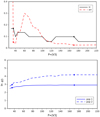 |
Fig. 3. Optimal values from the sampling parameter P = |W|. Top: entropy, H (dimensionless), and χ2 (scaled error). Bottom: trend of the vertical velocity dispersion σ3 (on a logarithmic scale). |
3.4. Kinematical parameters of the samples
In Appendix A, we justify in detail why the working sample is kinematically representative of the GP. Based on this fact, we may now extract conclusions about which subsamples provide us with information concerning the thin disc, the thick disc, or the halo.
Table 1 displays the characteristic parameters of the segregated components. The values for the thin disc are stable and consistent whether obtained from the sampling parameters |v| = 123 km s−1, |v| = 230 km s−1, and |W| = 35 km s−1. Similarly, the parameters of the whole disc are stable when obtained sampling parameters from |W| = 130 to 170 km s−1. On the contrary, for the thick disc and the halo, these values depend on the size of the sample, that is, on the fraction of stars included as population 2, which, in addition, have larger velocities and produce unstable values for these populations.
Hence, to define the boundaries between populations in terms of the eccentricities, the characteristic parameters for the thin-thick segregation are to be taken from the sampling parameter |v| = 230 km s−1 and for the segregation disc-halo, we use the sampling parameter |W| = 170 km s−1. Furthermore, for a more detailed characterisation of the subpopulations, in order to distinguish between the thin disc and the canonical thick disc, we use the values obtained for the sampling parameter |v| = 123; and in order to distinguish between the canonical thick disc and the MWTD, we use those obtained for |v| = 350.
4. Labelling the populations
4.1. The most likely population
Let us assume a sample Ω of stars consisting in a partition of disc and halo populations, Ω = D ∪ H, where the set of disc stars also consists in a partition of thin and thick disc populations, D = t ∪ T. Given the characteristic kinematic parameters of each stellar population, for a star s ∈ Ω we calculate the probability of belonging to the population, S, namely, π(s ∈ S).
Firstly, the segregation disc-halo is considered, from where we get the velocity distribution functions (trivariate Gaussian) for computing the probabilities of a star to belong to the disc π(s ∈ D) and to the halo π(s ∈ H), so that π(s ∈ D)+π(s ∈ H) = 1. Secondly, from the thin-thick disc segregation, for the stars likely belonging to the disc, we compute the probabilities of a star to belong to the thin disc π(s ∈ t|D) and to the thick disc π(s ∈ T|D), so that π(s ∈ t|D)+π(s ∈ T|D) = 1.
The easiest method, say L0, for labelling a star according to one of the populations is to assign the star to the more probable population. Thus, a star can be labelled as t, T, H, although this does not provide a relative scale among populations when, inevitably, cases arise where a star belongs to an area where the tails of two distributions overlap. For instance, it is possible that a thick-disc star has a higher probability of belonging to the thin disc, and then it is labelled incorrectly. Hence, there must be a mutual exchange of labels established between these stars. This should not be considered a major issue if the number of these stars is relatively low (such as the case of the thin disc), as generally occurs when the sample is large and the populations are significantly differentiated, but it is not negligible for the thick disc, with a relatively low number of stars.
However, once the respective populations have been withdrawn from the whole catalogue, as a consequence of having cut the wings of the distributions, the resulting partial samples will have lost the clock shape of the Gaussian distributions. If we compute their moments we obtain some modified distributions sharing the main basic trends, for instance, the means and the second moments, but with likely modified higher-order moments.
4.2. Population index
To determine if a star is in the overlapping region between populations or is in the most characteristic region of one of the populations, it is useful to have an index indicating, for each star, the expected value of the population the star belongs to. The index can also be used to extract more pure subsamples for a particular population. For this reason, we adopt two more approaches, which allow us to quantify with a population index the stars in relation to the populations. To each star, we assign a continuous value x(s) ∈ [0, 3] representing the expected population the star belongs to. Thus, the population index will be computed from three different methods:
L0. The simplest way for labelling a star is to assign the star a discrete value 1, 2, or 3 to x, depending on whether the most likely population is t, T, or H.
L1. The population index is computed as a continuous parameter from the expected value of a star to belonging to either of the three populations, labelled as x = 0 for the thin disc, x = 2 for the thick disc, and x = 3 for the halo, namely:

In this case, for the sake of continuity, the probabilities are obtained from the segregations with the same sampling parameter P = |v| for all the populations.
The value representing the average kinematics of the disc is x = 1. Within the disc, a star with a higher or equal probability of belonging to the thin disc satisfies 0 ≤ x ≤ 1, while stars satisfying 1 < x ≤ 2 have higher probability of belonging to the thick disc. Although values of x > 2 represent stars with higher probability of belonging to the halo than to the average disc, the range of 2 < x ≤ 2.5 still contains thick-disc stars, since these stars have higher probability of belonging to the thick disc than to the halo. Finally, the interval 2.5 < x ≤ 3 represents stars with higher probability of belonging to the halo. In the next subsection, we discuss the methods for labelling the populations in detail.
L2. We use the probabilities obtained from the sampling parameter P = |W| for the segregation disc-halo and the sampling parameter P = |v| for the segregation thin-thick discs. In this way, the separation of both main components disc-halo is emphasised. The value x(s) ∈ [0, 3] is computed in two different ways depending on whether the most likely population is the disc or the halo. Firstly, for the stars with higher probability of belonging to the disc, we compute the expected value x1 of belonging to the thin disc (label x1 = 0) or to the thick disc (label x1 = 2). Thus, x1 ∈ [0, 2] and, as with the previous method, the value of x1 = 1 represents the average disc as well as the limiting value between thin and thick disc. Secondly, for the stars with higher probability of belonging to the halo, we compute the expected value x2 of belonging to the disc (label x2 = 0) or to the halo (label x2 = 2). These stars satisfy x2 ∈ (1, 2]. Then, in order to produce a parameter x covering the total range [0, 3], the range of x2 is modified so that for the halo stars the interval is adjacent to the range of x1. Hence, the value x2 must be translated by 1. Therefore:

Now the disc and halo populations remain more isolated than in the previous case.
4.3. Comparing labelling methods
Here, we discuss these methods in detail. The approach marked as L1 considers the three populations as independent. For each star, the respective probabilities are:
which satisfy r = 1 − p − q. The possible values for p, q are displayed in Fig. 4, according to the following constraints between them, namely,
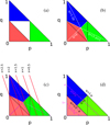 |
Fig. 4. Regions (a) of higher probability than the sum of the other populations for thin disc (green), thick disc (blue), and halo (light red). Regions of higher probability than each one of the other populations for cases L0 (b), L1 (c), and L2 (d). |
Panel a shows the coloured regions  (green),
  (blue), and
  (light red), where one of the probabilities is greater or equal than the sum of the others.
Panel b shows the coloured regions p ≥ q and p ≥ r (green), q ≥ p and q ≥ r (blue), r ≥ p and r ≥ q (light red), where one of the probabilities is greater than each one of the others. This is the case described as L0. However, in L1, it has been assigned the index x = 0p + 2q + 3r = 3 − 3p − q to each star. Therefore, the interval x ≤ α corresponds to the region q ≥ 3 − α − 3p. These are the limiting lines plotted in red in the panel c for values x = 0.5, 1, 1.5, 2, 2.5. These lines do not match the regions where each population has higher probability. Indeed, the regions 0 ≤ x ≤ 1 and 2.5 ≤ x ≤ 3 determine pure thin disc and halo stars, respectively, but the range 1 ≤ x ≤ 1.5 accounts for mixed stars labelled as thin and thick disc, and the range 1.5 ≤ x ≤ 2.5 accounts for mixed thick disc and halo stars. Therefore, although the parameter x has a desirable continuous behaviour for labelling the stars, it has a non negligible uncertainty.
An alternative approach for partially avoiding such a situation is to first consider the segregation disc-halo and, afterwards, within the disc, the segregation thin-thick disc. Such is the approach L2, which is represented in the panel d. For the segregation disc-halo, we consider the probabilities d = p + q = π(s ∈ D) and r = 1 − d = 1 − p − q = π(s ∈ H). The light-red region corresponds to probabilities  of halo stars, where
  . We refer to it as the halo region. The green and blue areas define the disc region, where the probability of disc stars is higher,
  , so that
  . In the halo region, a probability of
 ![Mathematical equation: $ r\in [\frac12,1] $](/articles/aa/full_html/2021/05/aa40017-20/aa40017-20-eq22.gif) defines the line q = (1 − r)−p, hence
defines the line q = (1 − r)−p, hence  . Since the index is computed as x = 1 + 2r, the line can be written in terms of x as
  for values 2 ≤ x ≤ 3.
Within the disc region, for a fixed value  , the respective probabilities of the thin and thick discs satisfy
  . Hence, q = d − p defines the line in the graph corresponding to this disc probability. Then, the index, that in this case has been evaluated as
  , corresponds to a point on this line of value
  . Along this line, the green zone satisfies q ≤ p and 0 ≤ x ≤ 1, while the blue zone satisfies q ≥ p and 1 ≤ x ≤ 2. In this approach, and comparing with panel b, we see that a small part of the halo can be mistaken as disc stars, but no disc stars are to be labelled as halo stars.
In order to interpret the resulting segregations and how they depend on the method, Figs. 5 and 6 display eccentricity, e, absolute velocity, |v|, maximum distance to the Galactic plane, zmax, and vertical eccentricity, e′, in terms of x (in grey, the percentage of stars according to the axis on the right), as well as the population index, x, in terms of the heliocentric velocities.
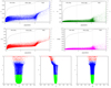 |
Fig. 5. Relation between several properties and the population index (x) for case L1. |
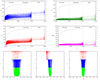 |
Fig. 6. Relation between several properties and the population index (x) for case L2. |
4.4. Subsamples
These labelling methods provide the following number of stars in each population:
-
L0
#t = 59 715 #T = 13 907 #H = 717.
-
L1
#t = 59 434 (0 ≤ x ≤ 1) #(t + T)+(T + H) = 3699 + 4832 = 8531 (1 < x ≤ 1.5 and 1.5 < x ≤ 2) #(T + H) = 5657 + 717 = 6374 (2 < x ≤ 2.5 and 2.5 < x ≤ 3).
-
L2
#t = 59 722 (0 ≤ x ≤ 1) #T = 12 357 (1 < x ≤ 2) #H = 2260 (2 < x ≤ 3).
The values for L0 and for L1 are computed from the samples with |v|< 230 km s−1 and |v|< 350 km s−1. As explained above, for the case of L1, in the range of 2 < x ≤ 3, there are many stars that likely belong to the thick disc.
For the case of L2, the listed values come from samples with |W|< 170 km s−1 for the segregation disc-halo, and |v|< 230 km s−1 for the segregation thin-thick disc.
The velocity moments of the samples containing thin disc and thick disc stars are listed at the end of the Appendix D. The moment values are nearly the same for all the labelling methods. For the thin-disc stars, the moments are similar to the first population obtained from the samples selected by |v|< 123, |v|< 230, and |W|< 35 km s−1. For the total disc they are similar to the total moments of the same samples.
4.5. Velocity distribution features
Firstly, we point out some basic features: (a) in the UV plane, the thin disc distribution is more ellipsoidal than the thick disc; (b) thin and thick disc distributions have a non-vanishing, although small, vertex deviation in the UV plane, while the halo does not have a significant one; (c) in the VW plane the disc populations have almost spherical distribution; (d) the mean velocities for the U and W velocity components are similar for the disc components and the inner halo, which is indicative of stationarity, so that the main difference between these populations takes place in the rotation velocity component.
More specific features are below described from Figs. 5 and 6, allowing us to compare methods L1 and L2. The main difference is due to the overlapping of thick-disc and halo populations that occurs for 2 < x < 2.5 in method L1 (as explained in Sect. 4). The method L2 produces a sudden change in x = 2, however, let us note that among the 12 357 stars with 1 < x ≤ 2, a total of 4101 satisfy 1.9 < x ≤ 2, which is nearly half of a thick disc. Similarly, among the 2260 stars with 2 < x ≤ 3, a total of 1226 satisfy 2.9 < x ≤ 3, which is the very core of the kinematical halo.
For method L1, with regard to the disc (0 ≤ x ≤ 2.5), in the range 0 ≤ x ≤ 2 the velocities, U and W, are symmetrically distributed around their mean. However, in the rotation component, V, the density of stars to the right of the mean is lower than to the left. This is specially remarkable in the range of 1 < x ≤ 2.5, corresponding to the part where the thick disc is dominant. That is the reason why stars in this range elicit a radial mean velocity that is significantly lower than the stars in the range of 0 ≤ x ≤ 1 and associated with the thin disc, resulting in a net asymmetrical drift between thin- and thick-disc stars.
Figures 7 and 8 are plotted to establish the velocity bounds for the population components. The population index x is plotted in terms of the heliocentric velocities. The population components are coloured in green for the thin disc, blue for the thick disc, and red for the halo.
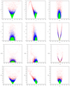 |
Fig. 7. Several properties in terms of the heliocentric velocities for case L1. |
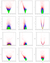 |
Fig. 8. Several properties in terms of the heliocentric velocities for case L2. |
For the whole disc, the velocity bounds are approximately (all velocities are given in km s−1):

For the thin disc, we get approximately:

These ranges are also valid for the graphs of method L2, Fig. 6.
For the halo (range 2.5 < x ≤ 3 in method L1 and 2 < x ≤ 3 in method L2), the above general features are repeated, although the asymmetry in rotation is emphasised. In particular, for case L1, this is a transitional region with a mixture of thick disc and halo stars. The drift in rotation is much higher than in the disc. There is a great lag in rotation, partially corresponding to a subcomponent with no net galactic rotation. For the halo, the velocity bounds are approximately

although most of them satisfy V ≤ −50.
Similarly, in Figs. 7 and 8 we are able to visualise the distribution of several properties in terms of the velocity components, such as the planar and vertical eccentricities (e and e′), the maximum height (zmax), and the absolute heliocentric velocity (|v|). These properties can be contrasted with the assigned population derived from the algorithm, indicated by the colour, to see whether they provide independent information about the stellar component the stars belong to.
We find that the U velocity component mixes up the populations when the eccentricities are taken into account, but it isolates the disc and the halo quite well in terms of the absolute heliocentric velocity. To display such a feature, the red points corresponding to the halo stars are plotted over those of the disc.
The V velocity component together with the planar eccentricity allow us to estimate the Galactocentric rotation velocity of the centroid in about 220−225 km s−1, which is consistent with the commonly accepted values (Kerr & Lynden-Bell 1986) and the Galactocentric rotation velocity of the Sun in about 225−230 km s−1. It is also possible to determine that the subset of stars that are symmetrically distributed around the centroid are those approximately satisfying e < 0.3. This is also evident from the plot of the absolute value of the heliocentric velocity, where the symmetry region corresponds to |v|≤50 km s−1. This interval size of ±50 km s−1 is maintained even while increasing the value up to approximately |v| = 140 km s−1. Then, as it goes up to |v| = 230 km s−1 or |v| = 250 km s−1, the interval of the V velocities becomes narrower, and afterwards it seems to expand again, as corresponding to two sub-halo components with opposite rotation. Similar features are deduced from the W component. In this case, the maximum interval size for a constant value |v| is reached approximately at |v| = 130 km s−1. For higher values, the size is maintained. Nevertheless, the planar eccentricity in terms of the W velocity is the only graph, among those of Figs. 7 and 8, that seems to isolate the three populations, with more accuracy between the whole disc and the halo. Therefore, it is reasonable to associate the slight overlapping between the thin and thick disc populations to some uncertainty in the labelling of the populations. Thus, we take advantage of this feature of such stellar properties for isolating regions of the graph. These regions, where one population is predominant, are not limited by constant values of these variables or by easily defined contours. We examine this fact in the following section. Since there exists a one-to-one relationship between the maximum height (or the vertical eccentricity) and the vertical velocity, which are linked through the potential (Eq. (C.1)), the graphs of Figs. 7 and 8 (first row and third column), where the previous relationship is depicted, suggest that the populations can be segregated exclusively in terms of the planar and vertical eccentricities.
5. Planar and vertical eccentricities
5.1. Epicycle approximation
In the attempt to devise better method for labelling the stars and to reduce the overlapping of the stellar populations of the sample, we used the epicycle approximation for disc stars (with the notation used in Cubarsi et al. 2017, hereafter Paper II). We consider the planar and vertical eccentricities as defined in Eqs. (2) and (3). To visualise the assignation of populations, we plot the eccentricities of each star (regardless whether they belong to the disc or not) versus the parameter x. In doing so, we obtain the graphs of Figs. 5 and 6, which depend on the labelling method. In these three cases, most of the thin disc stars (ca. 79−80% of the sample) have a planar eccentricity of 0 ≤ e ≤ 0.35; most of the thick disc stars (18−19% of the sample) have a planar eccentricity of 0 ≤ e ≤ 0.5; and most of the halo stars (2−4% of the sample) have a planar eccentricity of e > 0.5. We notice that the grey line indicating the cumulative percentage of population is consistent with the ranges of values of x assigned to each population. A similar analysis for the absolute velocity, the maximum distance zmax to the Galactic plane, and the vertical eccentricity e′ is also shown. From those graphs we see that most thin-disc stars satisfy |v|≤120 km s−1 (consistent with the sampling parameter |v| = 123 km s−1), zmax ≤ 1 kpc, and e′ ≤ 0.1.
Some of these features are similar to the segregation carried out from the relation between vertical and planar eccentricities of Paper I. For instance, for the method L2, which provides a reliable separation of disc and halo populations, the respective planar and perpendicular eccentricities determine two well-separated regions, which are more evident when plotting the squared eccentricities. However, thin and thick discs still end up partially overlapping.
It is widely recognised that the relationship between the eccentricities and the velocity components of the local circular motion point C at a given time t for each star can be written as (see, e.g., Eqs. (42), (43), and (46) of Paper II):
 (4)
(4)
 (5)
(5)
 (6)
(6)
Let us remember that the planar and vertical epicycle frequencies κ and ν are Galactic constants depending on the second derivatives of the potential (e.g., Binney & Tremaine 2008); a, b, φ, ψ are constants that are specific for each star, obtained from the initial conditions of position and velocity when integrating the equations of the star’s motion; and γc = 2Ωc κ−1 is a dimensionless constant depending on the angular velocity of C, which can be assumed constant around the radius rc (as justified in Paper II, Eq. (41)). Nevertheless, we go on to see that phases φ, ψ are not needed for our calculations.
Bearing in mind Eqs. (2) and (3), we get the following relationships between positive constants:
 (7)
(7)
As a first approximation, we assume that Uc = U0, Vc = V0 and Wc = W0, that is, the circular motion point coincides with the local centroid. For disc stellar samples, this assumption is generally satisfied in the radial and vertical directions. For the rotation component, a priory, it is satisfied for low eccentricity stars, that is, for thin-disc stars, otherwise the asymmetric drift Δ = Vc − V0 should be considered to get a more accurate model.
For a given planar eccentricity, e, we find stars in the sample with radial velocities of U − U0 ∈ [ − a, a] (e.g., Fig. 7, 1st row, 1st column) and stars with peculiar rotation velocity within the interval ![Mathematical equation: $ [- \kappa \gamma_{\mathrm{c}}^{-1} a,\; \kappa \gamma_{\mathrm{c}}^{-1} a] $](/articles/aa/full_html/2021/05/aa40017-20/aa40017-20-eq36.gif) around the mean rotation velocity V0, which depends on the stellar population they belong to, tending towards −220 km s−1 for the halo, or even lower values for the counter-rotating halo (e.g., Fig. 7, 1st row, 2nd column). We notice, however, that as the value V0 decreases, the eccentricity increases, and the number of stars in the sample decreases dramatically, so that at the corresponding eccentricity level, the graph becomes nearly empty.
around the mean rotation velocity V0, which depends on the stellar population they belong to, tending towards −220 km s−1 for the halo, or even lower values for the counter-rotating halo (e.g., Fig. 7, 1st row, 2nd column). We notice, however, that as the value V0 decreases, the eccentricity increases, and the number of stars in the sample decreases dramatically, so that at the corresponding eccentricity level, the graph becomes nearly empty.
For the vertical eccentricity and the vertical velocity component, by taking into account that the height of star referred to the GP is z = b sin(νt − ψ) and that our stellar sample is approximately on the GP, we have sin(νt − ψ)≈0 and cos(νt − ψ)≈ ± 1. Therefore, for a fixed vertical eccentricity, we may find stars with values W − W0 ≈ −νb or W ≈ νb, but not within these values, as shown in Figs. 7 and 8 (3rd row, 3rd column). Thus, in the GP, Eq. (6) becomes:
 (8)
(8)
However, the above graphs are not actually V-shaped. It is for this reason that the foregoing equation, associated with the epicycle approach, is replaced in Sect. 5.3.2 by a more general approximation.
5.2. Most likely population from eccentricities
To evaluate which population a star is most likely to belong to in terms of the planar and vertical eccentricities, we compare the probability density functions of two consecutive segregated populations (with regard to the order induced by the sampling parameter P), namely, thin disc versus thick disc, and disc versus halo.
Let us consider a star s with velocity v. We write the respective partial velocity density functions for two populations, S′ and S″, as f′(v)=π(v|S′) and f″(v)=π(v|S″), which are assumed to be Schwarzschild distributions. The total probability density function is obtained from superposition as f(v)=n′f′(v)+n″f″(v), where n′ = π(s ∈ S′) and n″ = π(s ∈ S″). According to the epicycle approximation, the respective partial velocity ellipsoids are aligned along their symmetry axes. In terms of the planar and vertical eccentricities, we want to determine the population component with with the highest probability. For instance, we want to see whether:
 (9)
(9)
Such a condition is derived in Appendix B, where we define:
 (10)
(10)
and we get Eq. (B.5), which can be expressed as:
 (11)
(11)
Alternatively, by taking into account Eq. (7) in terms of the eccentricities, we can also write:
 (12)
(12)
Since the velocity dispersions of the thin disc, thick disc, and halo increase progressively, that is,  and
and  , and their population fractions decrease, that is, n′> n″, the values of A, B, A0, B0, and Q are positive. In such a case, the two foregoing equations define a quarter ellipse. Alternatively, if we write Eq. (12) as:
 (13)
(13)
we get a triangle region for the squared eccentricities e2 and e′2. We refer to the last representation as an eccentricity diagram.
Figure 9 displays these regions, estimated from the population index for the labelling method L2. Despite the fact that the segregation was carried out from the velocities instead of the eccentricities, we can observe the tendency of the disc (green plus blue dots) and the halo (red dots) to separate. On the contrary, stars labelled as thin- and thick-disc clearly overlap. This is due to the labelling inaccuracy.
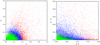 |
Fig. 9. Planar and vertical eccentricities (left) and squared eccentricities (right) of the stars labelled according to method L2 (green for thin disc, blue for thick disc, and red for halo). |
5.3. Determining the local constants
Several remarks must be made about the samples used to determine the local kinematic parameters of disc stars. If the 111 stars of the counter-rotating halo are included, that is, stars with V < −230 km s−1, the fitting for V0 is not reliable. It leads to a circular motion point with positive heliocentric rotation velocity – which does not make any sense. Even so, some stars still introduce a significant uncertainty, such as those with a likely erroneous heliocentric velocity greater than 500 km s−1. We find that all these unreliable stars are excluded when considering only the stars with a planar heliocentric velocity  km s−1.
The samples selected from the sampling parameter |W| always contain stars with great eccentricity for which the epicycle approximation is not valid. The reason can be deduced from the graph of Fig. 7 in the first row, third column, where we see that even for low values |W| the planar eccentricities can reach maximum values.
Nevertheless, the above remark supports the explanation of how the sampling parameter P = |W| exhibited the proper behaviour to segregate populations: the algorithm worked appropriately since there were enough stars in each population component to be segregated. Thus, the sampling parameter |W| = 35 provided a segregation of thin disc, on the one hand, and thick disc plus halo, on the other hand, although their distributions are slightly truncated, mainly those of the thick disc and the halo. Hence, the thin disc was rather well identified as population 1, although a partial thick disc and a partial halo (stars with higher eccentricities) remained mixed into population 2. For these reasons, the most representative samples of the disc to determine the local parameters are those selected from the absolute heliocentric velocity |v|.
5.3.1. Planar fitting
Firstly, we fit the linear relationship given of Eq. (B.2). Bearing in mind Eq. (7), we write it as:
 (14)
(14)
We use the estimation obtained by fitting e instead of the orbital amplitude, a, because the eccentricities of the stars in the sample are referred to by their circular velocity point, rc, and, in many cases, this value is far from r0. However, the ratio  always satisfies the condition e ≤ 1. Therefore, the planar eccentricities (linked to the planar epicycle frequency and to the angular rotation velocity, which, as commented above, are approximately constant in a wide region around r0) are marked by a condition that is homogeneous for all the stellar sample, regardless of whether rc is similar to or different from r0. Instead, if we use the orbital amplitude a, the local value of
  is unconstrained (and much greater than 1 for most halo stars) and has a great dispersion depending on the star’s value rc. This is illustrated in Fig. 10 via a comparison of the left and right plots.
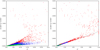 |
Fig. 10. Fitting by using the orbital amplitude a and (right) by using the planar eccentricity e (left). Fitting of Eq. (14) (continuous line) for disc stars, excluding the counter-rotating halo. |
The resulting parameters are listed in Table 2. They are very stable for the thin and thick discs, that is, with either of the samples containing stars with a population index 0 ≤ x ≤ α for 0.5 ≤ α ≤ 2.5 (method L2), as well as for samples selected as |v|≤50, |v|≤123. The fitting for disc stars is shown in Fig. 10 (continuous line) for values: Uc = −10 km s−1, Vc = −20 km s−1,  ,
,  km2 s−2.
We note that we get a value of  ≈ 2, which is consistent with the ratio μ11/μ22 ≈ 2 of the optimal sample selected from |v|≤230, containing mostly thin- and thick-disk stars. In Fig. 10 (right), we show the fitting obtained by excluding the stars with absolute velocity |v|> 500, the stars of the counter-rotating halo, V < −230, as well as the halo stars with a planar velocity
  .
.
By assuming r0 = rc = 8.3 kpc (Reid et al. 2014), which is the average value of the mean orbital radius of the stars in the sample, the values obtained from the population index yield a planar epicycle frequency κ = 36.9 ± 0.2 km s−1 kpc−1, which is consistent with the commonly assumed value (Binney & Tremaine 2008). The values for (Uc, Vc), match the mean velocities (U0, V0) obtained for the corresponding disc samples selected by P = |v| as well as P = |W| (tables in Appendix D) with an error of ±1. Hence, we can confirm the assumption that the local centroid is approximately in a circular orbit.
Furthermore, fitting from planar eccentricities means it is not necessary to estimate the asymmetric drift. In other words, we get a value, Vc, that matches the mean velocity, V0; whereas working with the orbital amplitude, the former value would differ from the latter depending on the asymmetric drift of the subsample. The reason for this is the following: the ellipses of Eq. (14) describe the motion of the stars referred to their circular velocity point, that is, their mean radius, say rm, which not always match the local one rc. However, the local constants γc and κ should not differ very much from point to point. On the one hand, the latter does not depend on rc. On the other hand, the former depends on the angular velocity of the circular velocity  , which, although it is not constant, satisfies the following (Paper II, Eq. (39)):
 (15)
(15)
Therefore, around the Sun,  . Hence, this variation is relatively small. Thus, the respective fittings, even for different circular velocity points, can be gathered as the same fitting.
5.3.2. Vertical fitting
Although the amplitude of the graph e vs. U − U0 varies linearly, it does not in the graph e′ versus W − W0, as shown in Fig. 7, second row, third column. Figure 11 shows that the approximation of linear dependence is valid only for small values of zmax and e′ for the core of the thin disc. The absolute value of the slope increases with higher values of zmax. When fitting the vertical motion, it occurs the opposite to the planar fitting. The vertical eccentricity of a star has been defined depending on the radius rc to which is referred its circular orbit. For the local stellar sample, rc covers a wide range around r0; then, for the same value zmax, we may get lower or higher vertical eccentricities. However, the vertical amplitude zmax is quite homogeneous among the stars in the sample, meaning that it is not sensitive to the mean orbital radius of the star. This fact that the vertical eccentricity is not appropriate for the vertical fitting, is illustrated in Fig. 11, where the graph on the left, plotted in terms of e′, shows a greater dispersion of dots (they form something similar to layers), especially for thick-disc and halo stars, than the graph on the right, plotted in terms of zmax. In Appendix C, we discuss this situation in detail. The graph on the right of Fig. 11 also depicts the biquadratic fit (grey continuous line) for
 (16)
(16)
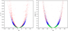 |
Fig. 11. Relation e′2 − W (left) and |

by using the average values obtained from the samples selected according to population index, corresponding to values c1 = 2.49 × 10⁻⁴ kpc2 s2 km−2, c2 = 4.99 × 10⁻⁸ kpc2 s4 km−4, Wc = −6.1 km s−1.
Hence, for these stars, the value ν corresponding to the ratio
 (17)
(17)
can be estimated as ν = 63.4 ± 0.1 km s−1 kpc−1, which is consistent with (although slightly lower than) the commonly assumed value of 70 (Binney & Tremaine 2008). The parameters are quite stable for different subsamples, as shown in Table 3.
5.4. Eccentricity diagram
5.4.1. Linear approximation
Firstly, we use the linear model of the epicycle approximation instead of the biquadratic fitting of Eq. (16) to carry out a test of the eccentricity diagram. By assuming rc = r0, we write Eq. (8) as:
 (18)
(18)
For the perpendicular motion, across the whole stellar sample, we use the estimation ν = 63.4 km s−1 kpc−1, which, according to Table 3 is shared by all the subsamples with 0 ≤ x ≤ 2.5. By assuming r0 = 8.3 kpc, we get  km2 s−2. For the planar motion, we use the estimations
  = 1.96 and
  km2 s−2, also approximately shared, according to Table 2, by all the subsamples with 0 ≤ x ≤ 2.5.
By taking into account the velocity moments and population fractions for the subsamples listed in Table 1 we determine the constants A0 and B0 for the limits of the triangular regions Ri listed in Table 4.
5.4.2. A more precise approximation
We now modify the model by taking into account the biquadratic approximation of Eq. (16), written as:
 (19)
(19)
where  and
and  . Then, the peculiar vertical velocity in terms of the vertical eccentricity may be written as:
 (20)
(20)
If q = 0 we get the linear relationship of Eq. (18). We note that the value
obtained in the current fitting yields a value α ≈ 55. On the other hand, e′2 can reach values close to 0.1. Therefore 4αe′2 is not always lesser than 1. Hence, Taylor expansions of the square root in Eq. (20) should be avoided. Thus, Eq. (12) becomes:
 (21)
(21)
The above equation is an area quite similar to the quarter ellipse of Eq. (12), but with the vertical semiaxis modified, as it is shown in Fig. 12, green and blue curves on the left. For e = 0, the maximum value ζ for the vertical eccentricity satisfies:
 (22)
(22)
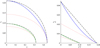 |
Fig. 12. Quarter ellipses (left) define the regions up to R2 (green line) and up to R4 (blue line) according to the biquadratic approximation: Eq. (21). The red dotted lines are for the linear model, Eq. (18). The black dashed lines are approximation of the biquadratic model by an ellipse, Eq. (23). Right: corresponding regions in terms of the squared eccentricities. |
Hence, Eq. (21) can be approximated as
 (23)
(23)
Equation (13) becomes modified and approximated in the same way as
 (24)
(24)
As displayed in Fig. 12, since the thin-disc stars (within the region limited by R2) have low eccentricities, the approximation of the biquadratic fit (green curve) by a modified ellipse (black dashed curve) does not introduces a significant error. For the whole disc (within the region limited by R4, blue curve), the error is greater, due to the thick-disc stars with higher eccentricities, although qualitatively, the approximated ellipse is still meaningful and easier to describe. In any case, both approximations are far better than the linear approach (red dotted lines). Thus, the triangular regions can be improved according to the values B1 listed in Table 4. The resulting eccentricity diagram, is shown in Fig. 13.
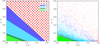 |
Fig. 13. Triangular regions according to Eq. (12) (left). The complementary area is the halo (red). Right: same plot for the actual stars in the sample. |
The stars can now be labelled according to the regions of the above diagram. The number of stars in a region, Ri, that do not belong to the regions, Rj, for j < i is denoted as Ni, and the corresponding population or subpopulation component as Pi. Thus,

The means and second central moments of these components are listed in Table 5.
Mean velocities, central moments, and population fractions (relative to the whole sample) for the populations and subpopulations obtained from the eccentricity diagram.
6. Discussion
There are two ways which allow us to check whether the regions selected from eccentricities instead of the population index depict the expected properties and, in particular, whether they isolate populations. One is the plot e in terms of W, suggested in the previous section. We see in Fig. 14 (left) that the populations remain well isolated, without overlapping areas. The other is shown in Fig. 14 (right), where the stars are labelled according to the eccentricity diagram instead of the population index from the methods L1 or L2. For each star we plot the quantity p(W − W0)2 + q(W − W0)4, expressed in Eq. (19), versus c1(U − U0)2 + c2(V − V0)2, from Eq. (14), by using the local constants obtained in the corresponding fittings, i.e., p, q, c1, and c2. The first three constants are equivalent to κ, γc and ν, while the latter measures the deviation from the linear model in the vertical component of the velocity. Therefore, with these local constants, the planar eccentricity and the vertical eccentricity can be used to determine the stars’ population. The loss of linearity in the vertical component of the epicycle model justifies the slightly convex shape of the contours separating the corresponding regions in the graph, which was predicted in Fig. 12 (right). Nevertheless, the approximate values for the maximum eccentricities that determine the respective regions can be estimated with enough accuracy from the corrected elliptical model given by Eq. (23).
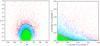 |
Fig. 14. Plot e versus W that isolates populations (left). Plot p(W − W0)2 + q(W − W0)4 versus c1(U − U0)2 + c2(V − V0)2 that isolates populations and reproduces the eccentricity diagram (right). |
The mean velocities and the second central moments of the subsamples selected by star eccentricities of Table 5 can be now compared to the values of Table 1 obtained from the MEMPHIS algorithm to identify the populations. The values for P1 + P2 are consistent with those of the thin disc t (population 1) obtained from the sampling parameters |v| = 123, |v| = 230, and |W| = 35 km s−1, although, in general, the method of eccentricities provides a slightly higher value for the moment μ020, which is compensated for by using a lower differential rotation velocity. Therefore, we can associate the triangular region up to R2 with the thin disc population8. We note that on the one hand, the subsample P1 has a moment μ002 still too low compared with the respective populations 1 of the mentioned samples to be considered the full thin disc. On the other hand, for the subsample P2, this moment is a bit short compared with the thick disc samples obtained as population 2 from the sampling parameters |v| = 230 and |v| = 350. Therefore, we should consider the stars of the subsample P2 as a tail of the thin disc that have a behaviour similar to the stars of a tail of the thick disc and, therefore, not an independent subpopulation.
For the same reasons, the subsamples P3 and P4 can be considered thick-disc samples. The heliocentric rotation velocity of about −57 km s−1 for the subsample P4 is consistent with that of the MWTD stars, which may vary between −120 and −50 km s−1, depending on the selected samples (e.g., Carollo et al. 2010; Ruchti et al. 2011; Kordopatis et al. 2013; Beers et al. 2014). Hence, subsample P3 can be associated with the canonical subcomponent and P4 with the MWTD. Nevertheless, it is worth noticing the difference in radial motion of about 9 km s−1 between these two subpopulations.
The values for P1 + P2 + P3 + P4 are similar to the total moments of the sample selected from |v|≤123, which contained the thin and thick discs, and are similar to the population 1 obtained from |W|≤170. Those values are slightly lower than the total moments of the samples selected from |v|≤230 and |v|≤350 (which may indicate that these ones are contaminated with halo stars). Furthermore, the values corresponding to the samples P1 + P2 + P3 (not shown in the table) match the ones of population 1 obtained for the sample |v|≤350, a finding that is consistent with the interpretation that the latter sample contains a mixture of thin-disc and canonical thick-disc stars. The samples limited by |W| = 130 and |v| = 350 yield a similar population 1, composed of thin-disc and canonical thick-disc stars.
With regard to P5, the moments are similar to those of the halo obtained from the sampling parameter |W| = 170 (in particular μ002). However, the rotation heliocentric velocity is significantly lower in the latter sample, while that of P5 is comparable to the one of population 2 from the samples selected as |v|≤350 and |W|≤35, which indicates that P5 still contains some MWTD stars mixed with the MRHD stars. It is not possible to be more precise with regard to this point, as among the few stars with |v|> 230, we find MWTD stars mixed with MRHD stars, with a few chemical halo stars (some of them belonging to the counter-rotating halo) and with stars with likely errors in their estimations. Hence, the parameters of the kinematical halo of our disc sample are only a wholesale estimation.
The mean metallicities [Fe/H] of these subsamples decrease from P1 to P5. The kinematical halo component P5 can be associated with the MRHD, in agreement with Di Matteo et al. (2019). With regard to the chemical halo stars having [Fe/H] < −1, the current sample only contains 565 stars satisfying such a condition. This set of stars does not conform an own (Gaussian) population, but together with the MRHD stars, they become one single component.
7. Conclusions
The combination of methods explained in this work has allowed us to characterise thin- and thick-disc stars in terms of their planar and vertical eccentricities with the help of the eccentricity diagram. In a first step, by using a local disc sample from the Gaia DR2 catalogue composed of 74 339 stars within a solar radius of 100 pc, we applied the MEMPHIS segregation algorithm to obtain the central velocity moments of its stellar population components (by associating each kinematical population with one Schwarzschild velocity distribution).
In Appendix A, we prove that the determination of the GP is quite accurate, with an error of ±20 pc, which might produce a maximum error of about ±1.3 km s−1 in the estimation of the vertical velocities. According to Table 1, we obtained the following velocity dispersions: for the thin disc (σ1, σ2, σ3)=(30, 14, 14) km s−1 (77% of the total sample), for the thick disc (σ1, σ2, σ3)=(53, 34, 31) km s−1 (21% of the total sample). Together, they form the disc, with (σ1, σ2, σ3)=(32, 19, 18) km s−1 (98% of the total sample), while the remaining halo stars have (σ1, σ2, σ3)=(110, 56, 57) km s−1 (2% of the total sample). Within the thick disc, two subcomponents are distinguished: one of them associated with the MWTD (Carollo et al. 2010, 2019) and the latter with non-Gaussian distribution.
As in our previous analyses from other catalogues (Cubarsi et al. 2010; Alcobé & Cubarsi 2005; Cubarsi & Alcobé 2004) we get a small but significant vertex deviation of the disc populations and subpopulations, although now they are accompanied by more accurate estimates. The differential mean radial motion between populations is very small, but non-null, for the thin disc and the canonical thick disc, 5 ± 2 km s−1, and it is more significant, namely, 9 ± 3 km s−1, between the canonical thick disc and the MWTD stars. The few stars of the kinematical halo composing our sample do not show a significant tilt nor vertex deviation of the velocity ellipsoid. However, they also maintain a difference of radial mean velocity of about 9 km s−1 with regard to the disc.
The dispersions for the thin disc are similar to those obtained by using the same segregation algorithm published in Alcobé & Cubarsi (2005) for a HIPPARCOS sample and in Cubarsi et al. (2010) for a GCS sample. However, they differ from those obtained by Anguiano et al. (2018) by using the Gaia DR1 catalogue with chemical labelling. As commented at the beginning, the concepts of stellar population from a chemical or a kinematical approach do not match, since a chemical population is not constrained by the shape of the velocity distribution, which is a condition for our model. For the remaining populations, the actual sample provides slightly lower dispersions, although the sampling parameters for the optimal segregations are similar. We attribute it to the different composition of the sample.
In terms of the orbital eccentricities, the thin disc and the whole disc are respectively associated with the following triangular regions:
If the couple (e, e′) ∈ A, the star can be considered to belong to the thin disc; if (e, e′) ∈ B A, the star can be considered to belong to the thick disc; otherwise, it is a star of the kinematical halo. These regions have been defined in a more exact way by taking into account Eq. (16), although, in such a case, the eccentricity diagram describes the above regions in a less simple way.
There are two main advantages of labelling the stars according to the method of eccentricities instead of the inference methods L1 and L2. One is that there are no overlapping areas. Of course, these regions depend on the kinematical parameters used to discriminate the populations. A change in these parameters will not provide a dramatic change, but it can determine a region with an uncertain classification. The other advantage is that at the border between these regions, there is no a concentration of stars, as it happened with the methods L1 and L2. Let us remember that for the method L2, the interval 1.9 < x ≤ 2 contained a half-thick disc. Instead, once it reached the average eccentricities (and maximum height) of the thin-disc distribution, the star density decreases rapidly as eccentricities decrease.
In a future work, we would like to justify and improve the approximation given by Eq. (16) for the vertical velocity curve expressed in Eq. (C.1). This can provide us with useful information about the local shape of the potential function, allowing us to replace this approximate formula by a more meaningful one.
Similarly, it would be interesting to deepen the study of the age-velocity dispersion relation through the stars’ orbital eccentricities. The power law σi ∝ tα, which can be fitted with αi ≃ 0.3 for the radial and rotation velocities, i = 1, 2 (e.g., Binney & Tremaine 2008), by assuming that the average epicycle energy of a disc’s stellar population is  led to a consideration of the sampling parameter P = |v| as highly correlated with the age t in Alcobé & Cubarsi (2005). This was related to the increasing radial velocity dispersion of disc stellar samples in terms of the sampling parameter P and the corresponding saturations of σ1 indicating that the thin disc or the thick disc populations were totally included in the sample. Now, the linear behaviour given by Eq. (14), when taking average values, leads to the relationship
  . Therefore, the average squared planar eccenricity of a disc stellar sample could be used as an estimate ⟨e2⟩∝t2α of the average age of its stars.
The epicycle approximation consists in to refer the orbit of a star near the GP to a reference frame with its centre in the position C of a star in the GP in circular motion with the same angular momentum integral.
The radial heliocentric velocity component U positive towards the GC, the heliocentric velocity component V positive in the direction of the Galactic rotation, and the velocity component W perpendicular to the GP and positive towards the north galactic pole.
A similar situation happened in the HIPPARCOS catalogue at |v| = 131 km s−1 (Alcobé & Cubarsi 2005). The resolution is now 1 km s−1.
A higher sampling parameter is responsible for a few stars with unreal velocity |v|> 500 or zmax > 100 kpc (i.e. the maximum value of |z|) introduce great sampling variances to the velocity moments, so that the resulting sample is not good enough to carry out a segregation.
The sample obtained from W = 170 km s−1 can be improved by just removing four stars with |v|> 500 km s−1, which are not reliable. This reduces the error of the central velocity moments of the halo population in about 50%, while the resulting partial moments and mean velocities do not sensibly change, similarly to the x values. The resulting sample provides total and partial velocity moments similar to the sample obtained from W = 130 km s−1, and provides a population 1 very similar to that of the sample limited by |v| = 350 km s−1. The bound |v|≤500 was also used in Paper I to filter the HIPPARCOS and the Geneva-Copenhagen Survey catalogues to avoid stars having an erroneous estimation of the velocity, perhaps greater than the escape velocity.
As expected, the kinematical halo population is identified in a very unstable way since the working sample contains a very small fraction of these stars.
As a general rule, the more reliable moment to depend on is μ020, since μ200 has greater sampling variance and μ020 is very sensible to the rotation velocity obtained from the mixture model.
This approach is valid if we assume an approximate Gaussian velocity distribution for the whole disc. If we assume that the disc is the mixture of two Gaussian distributions, this behaviour applies to each Gaussian component, where the differential mean vertical velocity is very small and proportional to z. Therefore, it is also a valid approximation for each population.
Acknowledgments
The work at the Astronomical Observatory of Belgrade was supported by the Ministry of Education, Science and Technological Development of the Republic of Serbia under grant 451-03-68/2020-14/200002.
References
- Alcobé, S., & Cubarsi, R. 2005, A&A, 442, 929 [NASA ADS] [CrossRef] [EDP Sciences] [Google Scholar]
- Anguiano, B., Majewski, S. R., Freeman, K. C., Mitschang, A. W., & Smith, M. C. 2018, MNRAS, 474, 854 [CrossRef] [Google Scholar]
- Beers, T. C., Norris, J. E., Placco, V. M., et al. 2014, ApJ, 794, 58 [NASA ADS] [CrossRef] [Google Scholar]
- Binney, J., & Tremaine, S. 2008, Galactic Dynamics: Second Edition (Princeton, USA: Princeton University Press) [Google Scholar]
- Carollo, D., Beers, T. C., Chiba, M., et al. 2010, ApJ, 712, 692 [NASA ADS] [CrossRef] [Google Scholar]
- Carollo, D., Chiba, M., Ishigaki, M., et al. 2019, ApJ, 887, 22 [NASA ADS] [CrossRef] [Google Scholar]
- Casetti-Dinescu, D. I., Girard, T. M., Korchagin, V. I., & van Altena, W. F. 2011, ApJ, 728, 7 [NASA ADS] [CrossRef] [Google Scholar]
- Chandrasekhar, S. 1942, Principles of Stellar Dynamics (New York, USA: Dover Publications) [Google Scholar]
- Cropper, M., Katz, D., Sartoretti, P., et al. 2018, A&A, 616, A5 [NASA ADS] [CrossRef] [EDP Sciences] [Google Scholar]
- Cubarsi, R. 1990, AJ, 99, 1558 [NASA ADS] [CrossRef] [Google Scholar]
- Cubarsi, R. 2010, A&A, 510, A103 [NASA ADS] [CrossRef] [EDP Sciences] [Google Scholar]
- Cubarsi, R. 2014a, A&A, 561, A141 [NASA ADS] [CrossRef] [EDP Sciences] [Google Scholar]
- Cubarsi, R. 2014b, A&A, 567, A46 [NASA ADS] [CrossRef] [EDP Sciences] [Google Scholar]
- Cubarsi, R. 2018, Kinematics and Dynamics of Galactic Stellar Populations (Newcastle upon Tyne, UK: Cambridge Scholars Publishing) [Google Scholar]
- Cubarsi, R., & Alcobé, S. 2004, A&A, 427, 131 [NASA ADS] [CrossRef] [EDP Sciences] [Google Scholar]
- Cubarsi, R., Alcobé, S., Vidojević, S., & Ninković, S. 2010, A&A, 510, A102 [NASA ADS] [CrossRef] [EDP Sciences] [Google Scholar]
- Cubarsi, R., Stojanović, M., & Ninković, S. 2017, Serb. Astron. J., 194, 33 [NASA ADS] [CrossRef] [Google Scholar]
- Dehnen, W., & Binney, J. J. 1998, MNRAS, 298, 387 [NASA ADS] [CrossRef] [Google Scholar]
- Di Matteo, P., Haywood, M., Lehnert, M. D., et al. 2019, A&A, 632, A4 [NASA ADS] [CrossRef] [EDP Sciences] [Google Scholar]
- Erickson, R. R. 1975, ApJ, 195, 343 [NASA ADS] [CrossRef] [Google Scholar]
- ESA 1997, in The Hipparcos and Tycho Catalogues. Astrometric and Photometric Star Catalogues Derived from the ESA Hipparcos Space Astrometry Mission (Noordwijk, Netherlands: ESA Publications Division), Spec. Publ., 1200 [Google Scholar]
- Famaey, B., Jorissen, A., Luri, X., et al. 2005, A&A, 430, 165 [NASA ADS] [CrossRef] [EDP Sciences] [Google Scholar]
- Famaey, B., Pont, F., Luri, X., et al. 2007, A&A, 461, 957 [NASA ADS] [CrossRef] [EDP Sciences] [Google Scholar]
- Gaia Collaboration (Brown, A. G. A., et al.) 2016, A&A, 595, A2 [NASA ADS] [CrossRef] [EDP Sciences] [Google Scholar]
- Gaia Collaboration (Brown, A. G. A., et al.) 2018, A&A, 616, A1 [NASA ADS] [CrossRef] [EDP Sciences] [Google Scholar]
- Gaia Collaboration (Brown, A. G. A., et al.) 2021a, A&A, 649, A1 [NASA ADS] [CrossRef] [EDP Sciences] [Google Scholar]
- Gaia Collaboration (Smart, R. L., et al.) 2021b, A&A, 649, A6 [EDP Sciences] [Google Scholar]
- Galli, P. A. B., Loinard, L., Bouy, H., et al. 2019, A&A, 630, A137 [NASA ADS] [CrossRef] [EDP Sciences] [Google Scholar]
- Gilmore, G., King, I., van der Kruit, P. C., et al. 1990, The Milky Way as a Galaxy: Saas-Fee Advanced Course No. 19, Lecture Notes, Swiss Society of Astrophysics and Astronomy (University Science Books) [Google Scholar]
- Haywood, M., Di Matteo, P., Lehnert, M., et al. 2018, A&A, 618, A78 [NASA ADS] [CrossRef] [EDP Sciences] [Google Scholar]
- Holmberg, J., Nordström, B., & Andersen, J. 2007, A&A, 475, 519 [NASA ADS] [CrossRef] [EDP Sciences] [MathSciNet] [Google Scholar]
- Holmberg, J., Nordström, B., & Andersen, J. 2009, A&A, 501, 941 [NASA ADS] [CrossRef] [EDP Sciences] [Google Scholar]
- Katz, D., Sartoretti, P., Cropper, M., et al. 2019, A&A, 622, A205 [NASA ADS] [CrossRef] [EDP Sciences] [Google Scholar]
- Kerr, F. J., & Lynden-Bell, D. 1986, MNRAS, 221, 1023 [NASA ADS] [CrossRef] [Google Scholar]
- Kordopatis, G., Gilmore, G., Wyse, R. F. G., et al. 2013, MNRAS, 436, 3231 [NASA ADS] [CrossRef] [Google Scholar]
- Lindegren, L., Hernández, J., Bombrun, A., et al. 2018, A&A, 616, A2 [NASA ADS] [CrossRef] [EDP Sciences] [Google Scholar]
- Lynden-Bell, D. 1967, MNRAS, 136, 101 [NASA ADS] [CrossRef] [Google Scholar]
- Miyachi, Y., Sakai, N., Kawata, D., et al. 2019, ApJ, 882, 48 [NASA ADS] [CrossRef] [Google Scholar]
- Miyamoto, M., & Nagai, R. 1975, PASJ, 27, 533 [NASA ADS] [Google Scholar]
- Moni Bidin, C., Carraro, G., & Méndez, R. A. 2012, ApJ, 747, 101 [NASA ADS] [CrossRef] [Google Scholar]
- Ninković, S. 1992, Ap&SS, 187, 159 [Google Scholar]
- Ninković, S. 2018, Acta Astron., 68, 301 [Google Scholar]
- Nordström, B., Mayor, M., Andersen, J., et al. 2004, A&A, 418, 989 [NASA ADS] [CrossRef] [EDP Sciences] [Google Scholar]
- Ogorodnikov, K. F. 1965, Dynamics of Stellar Systems (Oxford, UK: Pergamon Press) [Google Scholar]
- Pasetto, S., Grebel, E. K., Zwitter, T., et al. 2012a, A&A, 547, A70 [NASA ADS] [CrossRef] [EDP Sciences] [Google Scholar]
- Pasetto, S., Grebel, E. K., Zwitter, T., et al. 2012b, A&A, 547, A71 [NASA ADS] [CrossRef] [EDP Sciences] [Google Scholar]
- Reid, M. J., Menten, K. M., Brunthaler, A., et al. 2014, ApJ, 783, 130 [Google Scholar]
- Ruchti, G. R., Fulbright, J. P., Wyse, R. F. G., et al. 2011, ApJ, 737, 9 [NASA ADS] [CrossRef] [Google Scholar]
- Siebert, A., Williams, M. E. K., Siviero, A., et al. 2011, AJ, 141, 187 [NASA ADS] [CrossRef] [Google Scholar]
- Skuljan, J., Hearnshaw, J. B., & Cottrell, P. L. 1999, MNRAS, 308, 731 [Google Scholar]
- Smith, M. C., Evans, N. W., & An, J. H. 2009a, ApJ, 698, 1110 [NASA ADS] [CrossRef] [Google Scholar]
- Smith, M. C., Evans, N. W., Belokurov, V., et al. 2009b, MNRAS, 399, 1223 [NASA ADS] [CrossRef] [Google Scholar]
- Soubiran, C., & Girard, P. 2005, A&A, 438, 139 [NASA ADS] [CrossRef] [EDP Sciences] [Google Scholar]
- Soubiran, C., Jasniewicz, G., Chemin, L., et al. 2018, A&A, 616, A7 [NASA ADS] [CrossRef] [EDP Sciences] [Google Scholar]
- Steinmetz, M. 2012, Astron. Nachr., 333, 523 [NASA ADS] [CrossRef] [Google Scholar]
- Steinmetz, M., Zwitter, T., Siebert, A., et al. 2006, AJ, 132, 1645 [Google Scholar]
- Sysoliatina, K., Just, A., Koutsouridou, I., et al. 2018, A&A, 620, A71 [NASA ADS] [CrossRef] [EDP Sciences] [Google Scholar]
- Zwitter, T., Siebert, A., Munari, U., et al. 2008, AJ, 136, 421 [NASA ADS] [CrossRef] [Google Scholar]
Appendix A: Considering whether the sample is representative of the GP
The purpose of this section is to analyse how the velocity moments depend on the determination of the GP and how these moments might indicate that we are dealing with a GP representative stellar sample. The second central moment most affected by a bad determination of the GP is μ002 = ⟨(W − W0)2⟩ (brackets denote mean values). The key question is whether its actual value accounts for the true value on the GP or whether it becomes slightly modified since most of the stars in the stellar sample could be placed a bit over the GP, say 0.1 kpc. A necessary correction of such a value can be interpreted in two ways:
(a) It can be assumed that we actually work with a sample taken basically from the GP but the covariances are computed with regard to an erroneous mean. The centroid velocity, W0, may be inexact due to a biased kinematic behaviour of some stars. For instance, the sample limited by |W|< 35 (heliocentric velocities) yields a value W0 = −5.7, whilst the sample satisfying |W|< 170 produces a value of W0 = −7.7 km s−1. In such a case, if the vertical centroid velocity at the GP is W1 instead of the measured value W0, then, the corresponding second moment should be:
![Mathematical equation: $$ \begin{aligned} \langle (W-W_1)^2\rangle&= \langle [(W-W_0) + (W_0-W_1)]^2\rangle \\&=\langle (W-W_0)^2\rangle -(W_0-W_1)^2. \end{aligned} $$](/articles/aa/full_html/2021/05/aa40017-20/aa40017-20-eq80.gif)
Thus, we should correct the moment with regard to an amount corresponding to the difference (ΔW)2 = (W0 − W1)2. According to the epicycle approximation, such a difference, in z = 0, is related to a difference in the height over the GP Δz, such that (ΔW)2 ≈ ν2(Δz)2. If |Δz|≲0.1, then |ΔW|≲7. In this case, the correction of the moment may be estimated in less than 50 km2 s−2.
(b) Alternatively, we may assume that the sample is slightly displaced from the GP. In such a case we will use the dependency of the moments in terms of the position (r, z) provided by the Chandrasekhar model, where the velocity distribution is, by hypothesis, quadratic in the peculiar velocities (in our case, trivariate Gaussian). Such relationships and their gradients are given in Cubarsi (2014a). We only need the following ones:
where the k’s are positive constants. Then, by setting the notation of  as the value at the GP, corresponding to z = 0, it satisfies:

Therefore, we have9
The factor  has an order of magnitude of −2 and the moment μ101 clearly vanishes with regard to its sampling variance for all the working samples as well as for their segregated populations. In any case, for the working samples, we have an order of magnitude of 1. Therefore, the variation of the moment μ002 is at most of few units, similar to its sampling variance. Then, we should abandon the interpretation of case (b).
We have other resources to test whether we are working with a GP sample, assuming that the GP is a symmetry plane for the velocity distribution. If we take a kinematical representative sample, such as the one limited by |v|< 350 (which excludes some anomalous stars and contains the entire disc), we can check the symmetry about z = 0 from the moments with odd powers in the vertical peculiar velocity. As seen above, the moment μ101 is clearly null. The moment μ011 is slightly different from zero, although very low, which is still possible in an axisymmetric model (Cubarsi 1990) where the mean velocities would not be even functions of z. Therefore, this may suggest a small (local) break in the assumption of a symmetry plane. The third moments μ201 and μ021 vanish (within 2σ error) and μ003 is very small (−738 ± 312). These moments, at z = 0, should vanish.
According to case (a), let us estimate the possible deviation from the GP, by assuming that W1 (different from W0) should be the exact mean vertical velocity in the GP. We assume that U0 and V0 are the mean radial and rotation velocities in the GP, which are provided without a significant error by our sample. We also assume that the planar and vertical velocity distributions are independent (which is quite true, since the only significant non-vanishing non-diagonal moment is μ110, responsible for a small vertex deviation). Thus,
![Mathematical equation: $$ \begin{aligned} {\mu _{201}^\mathrm{GP}}&= \langle (U-U_0)^2(W-W_1)\rangle \\&= \langle (U-U_0)^2 [(W-W_0)+ (W_0-W_1)]\rangle = \mu _{201}+\mu _{200}\Delta W. \end{aligned} $$](/articles/aa/full_html/2021/05/aa40017-20/aa40017-20-eq86.gif)
Hence,
 (A.1)
(A.1)
Similarly,
![Mathematical equation: $$ \begin{aligned} {\mu _{021}^\mathrm{GP}}&= \langle (V-V_0)^2(W-W_1)\rangle \\&= \langle (V-V_0)^2 [(W-W_0) + (W_0-W_1)]\rangle =\mu _{021}+\mu _{020}\Delta W \end{aligned} $$](/articles/aa/full_html/2021/05/aa40017-20/aa40017-20-eq88.gif)
Hence,
 (A.2)
(A.2)
Finally,
![Mathematical equation: $$ \begin{aligned} {\mu _{003}^\mathrm{GP}}&= \langle (W-W_1)^3\rangle = \langle [(W-W_0) + (W_0-W_1)]^3 \rangle \\&= \mu _{003}+3 \mu _{002}\Delta W -2 (\Delta W)^3. \end{aligned} $$](/articles/aa/full_html/2021/05/aa40017-20/aa40017-20-eq90.gif)
This is a depressed cubic equation in ΔW,  , with roots
 (A.3)
(A.3)
Since, for the working samples, we have μ021 ≲ 0, μ201 ≲ 0, and μ003 ≲ 0, from the above equations we must conclude,
 (A.4)
(A.4)
These quotients provide us with values of 0.6 ± 0.3, 1.3 ± 0.8, 3.9 ± 1.6, respectively. By assuming a possible error within 2σ, the three quotients would be satisfied altogether if ΔW is between 0.6 and 1.3 km s−1.
In summary, a correction of μ002 by a quantity (ΔW)2 of a one or two units can be carried out, but this is not necessary since it is similar to its sampling variance. We can safely affirm that we are working with a sample basically drawn from the GP.
An error of 100 pc in the GP, associated with a value ΔW = 7, would produce moments μ201 = −ΔWμ200 ≈ 9000, μ021 = −ΔWμ020 ≈ 4900, and μ003 = −2ΔWμ002 ≈ 5300, which are between 5 and 10 times greater than the actual values. Therefore, the error in the determination of the GP, by taking the maximum estimate ΔW = 1.3, should not be greater than 20 pc.
A non-null value for the moment μ011 would indicate that, locally, there is a slight asymmetry of the velocity distribution with respect to the GP. However, when the segregation disc-halo is carried out, such a moment is nearly null for the disc (7.5 ± 6) and also for the MRHD plus the inner halo (−2 ± 98). The total moment (−19.6 ± 3) is basically due to the differential velocities,

since the difference  is not null. The mean value for the disc is
  , which is a value similar to that of the local centroid. Nevertheless, the mean value for the halo is
  if the segregation is carried out from the sample limited by |W| = 170. This would suggest that the vertical velocity distribution of the halo stars contained in the working sample is not symmetric about the GP. Such a correction in about 4−6 km s−1, should be only applied to the halo, and would be associated with an error Δz of about 60−85 pc. However, the halo is scarcely representative in our sample and is the less reliable component.
Appendix B: Condition for most likely population
Equation (9) can be explicitly written as:
 (B.1)
(B.1)
According to the epicycle approximation via Eqs. (4), (5), and (8), we have:
 (B.2)
(B.2)
 (B.3)
(B.3)
and it approximately satisfies (Paper II, Eq. (61)):
so that by taking logarithms and simplifying the equation, we write Eq. (B.1) as
 (B.4)
(B.4)
By using the parameters defined in Eq. (10), and rearranging terms, we get the following condition:
 (B.5)
(B.5)
which involves the star amplitudes a and b instead of its velocities.
Appendix C: Errors in fitting the vertical eccentricities
There is a behaviour related to the vertical eccentricities that affects the stars but not always in the same way, as shown Fig. 11 (left), where the stars indexed as halo (red) define an inner and more convex curve to that of the disc stars.
Locally, the value of the vertical epicycle frequency ν can be assumed as constant. However, the solar sample contains many stars with a mean orbital radius rc between 4 and 6 kpc, so that they come from a far inner region of the Galaxy (there are also many stars with rc > r0, but they are less problematic). Even without considering that these stars might be oscillating according to a slightly different vertical epicycle frequency associated with the circular velocity point far from r0, when their orbits reach the solar position at the local circular velocity point r0, we come to assume the values e, e′, and zmax that have been obtained from an approximated potential at rc instead of r0. With these values it is possible to have some deviations from the model.
A more detailed analysis, displayed in Fig. C.1 (left), shows that the stars escaping the main trend are those with rc more distant to the solar radius r0. This is more important for the stars with rc < r0 than for rc > r0. If the maximum height is referred to r0 (Fig. C.1, right), the dispersion is lower. There are also some non-reliable stars that can be removed to lessen the dispersion, such as those with zmax > 15, |v|> 500, |W|> 170, and minimum distance to the GC rp < 0.1.
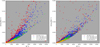 |
Fig. C.1. Dots plotted in terms of distances |rc − r0| with the maximum height referred to rc (left) and to r0 (right). |
When passing through the GP, all the stars have attained maximum vertical speed. There is one relationship between zmax and W at z = 0, given by the potential 𝒰 at r0 once integrated the third equation of motion,  . We refer to it as the maximum velocity curve:
 (C.1)
(C.1)
Thus, such a great dispersion shown in the previous graphs (except small dispersions allowed by some measurement errors) makes no sense. Since the values of W are solely based on observational data, we cannot change them. We should conclude that the estimations of zmax and, especially, e′ have some deviations from the values they should attain at the local radius, because they are estimated at values rc, different from r0.
We analyse the errors in fitting:
 (C.2)
(C.2)
Without taking into account any specific model for the potential, simply by using the fit, in a first approximation, by differentiating the above expression, we get  . Let us take b = zmax. Since the squared vertical eccentricity for a star with a circular orbit with radius r is
  , then
  , so that,
  . Since the velocities must always be lower than the velocity measured at the GP, by defining
  , we may estimate:
Thus, we should translate the curve for the vertical eccentricities with regard to the solar radius r0 in a quantity:
 (C.3)
(C.3)
We note that the value φ(w2) varies from 1 to  as w varies from 0 to ∞.
There are still three possible errors to consider: (a) the error due to a bad estimation of the Galactic plane (GP) z = 0; (b) the error in determining the maximum height zmax; and (c) the error due to a bad determination of the W velocity. To study these errors we assume a linear propagation of the error according to the epicycle approximation. Then, the variables z and w satisfy (e.g., Paper II, Eqs. (21) and (43)),
 (C.4)
(C.4)
The error due to a bad determination of the GP is obtained by differentiating Eq. (C.4), assuming a b constant. Thus, the error propagation corresponds to:

Since the local sample contains stars within a radius of 0.1 pc, we may assume a maximum error of Δz2 = 0.22. That is, by assuming ν = 70, Δw2 ≈ 200.
On the other hand, the same variation in w2 at z = 0 (see Fig. C.2) can be interpreted as an error in z2 for constant b2, or as an error in b2 under a correct determination of the GP. Hence, we assume that, at worst, an erroneous determination of Δb2 produces an error of Δw2 that is similar to the error due to the determination of the GP.
Now, we determine how the error due to a bad determination of the velocities, Δw2, is translated to e′2. Let us assume a relative error  , hence
  .
.
Thus, to Eq. (C.3) we must add these three possible errors, as follows,
![Mathematical equation: $$ \begin{aligned} \Delta {e}^{\prime 2}= (a_1 +2a_2 { w}^2) \Delta { w}^2= 2 (a_1 +2a_2 { w}^2)\; \left[\Delta z^2+ { w}^2 \beta + { w}^2 \varphi ({ w}^2) \frac{\Delta r}{r_0}\right]\cdot \end{aligned} $$](/articles/aa/full_html/2021/05/aa40017-20/aa40017-20-eq119.gif) (C.5)
(C.5)
The impact of these errors can be seen in Fig. C.3. The red line accounts for the error due to the term Δz2. Between the black and the red lines, we can see most of the thin-disc stars and a large share of the thick-disc stars. The blue line corresponds to a value of β = 0.2. Although it seems excessive to assume an error of 20% in the determination of the W velocities, there are still a lot of disc stars excluded from this explanation. Clearly, the prevailing error is the one associated with the different rc for each star, corresponding to the orange line. The addition of all the errors is represented in the grey line, which explains the dispersion of the dots. For this reason, we fit the curve Eq. (16) instead of Eq. (C.2).
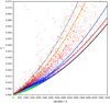 |
Fig. C.3. Maximum vertical velocity at r0 (black), the errors for the determination of the GP and the maximum height (red), an estimation of 20% relative error in the velocity (blue), an estimation of 50% relative variation around the radius r0 (orange), and the sum of all the errors (grey). |
Appendix D: Tables of moments
Moments for 72 859 stars with |v|≤123 km s−1.
Moments for 74 153 stars with |v|≤230 km s−1.
Moments for 74 272 stars with |v|≤350 km s−1.
Moments for 67 513 stars with |W|≤35 km s−1.
Moments for 74 332 stars with |W|≤170 km s−1.
Moments for 59 434 thin disc stars (0 ≤ x ≤ 1) from method L1.
Moments for 14 188 thick disc stars (1 < x ≤ 2.5) from method L1.
Moments for 73 622 disc stars (0 ≤ x ≤ 2.5) from method L1.
Moments for 59 722 thin disc stars (0 ≤ x ≤ 1) from method L2.
Moments for 12 357 thick disc stars (1 < x ≤ 2) from method L2.
Moments for 72 079 disc stars (0 ≤ x ≤ 2) from method L2.
All Tables
Mean velocities (km s−1), second central moments (km2 s−2), population fractions (relative to the subsample), and number of stars in terms of the sampling parameter P (km s−1) for optimal segregations.
Mean velocities, central moments, and population fractions (relative to the whole sample) for the populations and subpopulations obtained from the eccentricity diagram.
All Figures
|
Fig. 1. Local optimal values of the partition entropy, H (dimensionless), and χ2 (scaled error) obtained from the sampling parameter P = |v| inside the thin disc. |
| In the text | |
|
Fig. 2. Optimal values from the sampling parameter P = |v| (km s−1). Top: entropy, H (dimensionless), and χ2 (scaled error). Bottom: trend of the radial velocity dispersion σ1 (on a logarithmic scale). |
| In the text | |
|
Fig. 3. Optimal values from the sampling parameter P = |W|. Top: entropy, H (dimensionless), and χ2 (scaled error). Bottom: trend of the vertical velocity dispersion σ3 (on a logarithmic scale). |
| In the text | |
|
Fig. 4. Regions (a) of higher probability than the sum of the other populations for thin disc (green), thick disc (blue), and halo (light red). Regions of higher probability than each one of the other populations for cases L0 (b), L1 (c), and L2 (d). |
| In the text | |
|
Fig. 5. Relation between several properties and the population index (x) for case L1. |
| In the text | |
|
Fig. 6. Relation between several properties and the population index (x) for case L2. |
| In the text | |
|
Fig. 7. Several properties in terms of the heliocentric velocities for case L1. |
| In the text | |
|
Fig. 8. Several properties in terms of the heliocentric velocities for case L2. |
| In the text | |
|
Fig. 9. Planar and vertical eccentricities (left) and squared eccentricities (right) of the stars labelled according to method L2 (green for thin disc, blue for thick disc, and red for halo). |
| In the text | |
|
Fig. 10. Fitting by using the orbital amplitude a and (right) by using the planar eccentricity e (left). Fitting of Eq. (14) (continuous line) for disc stars, excluding the counter-rotating halo. |
| In the text | |
|
Fig. 11. Relation e′2 − W (left) and |
| In the text | |
|
Fig. 12. Quarter ellipses (left) define the regions up to R2 (green line) and up to R4 (blue line) according to the biquadratic approximation: Eq. (21). The red dotted lines are for the linear model, Eq. (18). The black dashed lines are approximation of the biquadratic model by an ellipse, Eq. (23). Right: corresponding regions in terms of the squared eccentricities. |
| In the text | |
|
Fig. 13. Triangular regions according to Eq. (12) (left). The complementary area is the halo (red). Right: same plot for the actual stars in the sample. |
| In the text | |
|
Fig. 14. Plot e versus W that isolates populations (left). Plot p(W − W0)2 + q(W − W0)4 versus c1(U − U0)2 + c2(V − V0)2 that isolates populations and reproduces the eccentricity diagram (right). |
| In the text | |
|
Fig. C.1. Dots plotted in terms of distances |rc − r0| with the maximum height referred to rc (left) and to r0 (right). |
| In the text | |
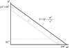 |
Fig. C.2. Relationship between errors in z2, b2, and w2 from Eq. (C.4). |
| In the text | |
|
Fig. C.3. Maximum vertical velocity at r0 (black), the errors for the determination of the GP and the maximum height (red), an estimation of 20% relative error in the velocity (blue), an estimation of 50% relative variation around the radius r0 (orange), and the sum of all the errors (grey). |
| In the text | |
Current usage metrics show cumulative count of Article Views (full-text article views including HTML views, PDF and ePub downloads, according to the available data) and Abstracts Views on Vision4Press platform.
Data correspond to usage on the plateform after 2015. The current usage metrics is available 48-96 hours after online publication and is updated daily on week days.
Initial download of the metrics may take a while.