| Issue |
A&A
Volume 646, February 2021
|
|
|---|---|---|
| Article Number | A5 | |
| Number of page(s) | 11 | |
| Section | Interstellar and circumstellar matter | |
| DOI | https://doi.org/10.1051/0004-6361/202039611 | |
| Published online | 02 February 2021 | |
Gas phase Elemental abundances in Molecular cloudS (GEMS)
III. Unlocking the CS chemistry: the CS+O reaction
1
Department of Physics, University of Firat,
23169 Elazig, Turkey
2
Instituto de Física Fundamental (IFF-CSIC), C.S.I.C.,
Serrano 123,
28006 Madrid, Spain
e-mail: octavio.roncero@csic.es
3
Departamento de Química-Física Aplicada, Unidad asociada IFF-UAM, Universidad Autónoma de Madrid
28049, Spain
4
Institut des Sciences Moléculaires ISM), CNRS, Univ. Bordeaux,
351 cours de la Libération,
33400 Talence, France
5
Observatorio Astronómico Nacional (OAN-IGN),
c/ Alfonso XII 3,
28014 Madrid, Spain
6
Laboratoire d’astrophysique de Bordeaux, Univ. Bordeaux, CNRS, B18N, allée Geoffroy Saint-Hilaire,
33615 Pessac, France
7
Sorbonne Université, Observatoire de Paris, Université PSL, CNRS, LERMA,
92190
Meudon, France
8
Center for Astrophysics | Harvard & Smithsonian,
60 Garden St.,
Cambridge,
MA 02138, USA
9
Centre for Astrochemical Studies, Max-Planck-Institute for Extraterrestrial Physics,
Giessenbachstrasse 1,
85748
Garching, Germany
10
Centro de Astrobiología (CSIC-INTA), Ctra. de Ajalvir, km 4, Torrejón de Ardoz,
28850 Madrid, Spain
11
Instituto Radioastronomía Milimétrica (IRAM),
Av. Divina Pastora 7,
Nucleo Central,
18012
Granada, Spain
12
Observatorio de Yebes (IGN),
Cerro de la Palera s/n,
19141 Yebes,
Guadalajara, Spain
13
Department of Space, Chalmers University of Technology, Earth and Environment,
412 93 Gothenburg, Sweden
14
Faculty of Aerospace Engineering, Delft University of Technology, Delft, University of Leiden,
PO Box 9513, 2300 RA Leiden, The Netherlands
15
École Normale Supérieure de Lyon, CRAL, UMR CNRS 5574, Université Lyon I,
46 allée d’Italie,
69364,
Lyon Cedex 07, France
16
Jeremiah Horrocks Institute, University of Central Lancashire,
Preston PR1 2HE, UK
17
Department of Physics, University of Helsinki,
PO Box 64,
00014 Helsinki, Finland
18
Institute of Physics I, University of Cologne,
Cologne, Germany
19
National Radio Astronomy Observatory,
520 Edgemont Rd.,
Charlottesville VA 22901, USA
20
Leiden Observatory, Leiden University,
PO Box 9513,
2300 RA Leiden, The Netherlands
Received:
7
October
2020
Accepted:
10
December
2020
Context. Carbon monosulphide (CS) is among the most abundant gas-phase S-bearing molecules in cold dark molecular clouds. It is easily observable with several transitions in the millimeter wavelength range, and has been widely used as a tracer of the gas density in the interstellar medium in our Galaxy and external galaxies. However, chemical models fail to account for the observed CS abundances when assuming the cosmic value for the elemental abundance of sulfur.
Aims. The CS+O → CO + S reaction has been proposed as a relevant CS destruction mechanism at low temperatures, and could explain the discrepancy between models and observations. Its reaction rate has been experimentally measured at temperatures of 150−400 K, but the extrapolation to lower temperatures is doubtful. Our goal is to calculate the CS+O reaction rate at temperatures <150 K which are prevailing in the interstellar medium.
Methods. We performed ab initio calculations to obtain the three lowest potential energy surfaces (PES) of the CS+O system. These PESs are used to study the reaction dynamics, using several methods (classical, quantum, and semiclassical) to eventually calculate the CS + O thermal reaction rates. In order to check the accuracy of our calculations, we compare the results of our theoretical calculations for T ~ 150−400 K with those obtained in the laboratory.
Results. Our detailed theoretical study on the CS+O reaction, which is in agreement with the experimental data obtained at 150–400 K, demonstrates the reliability of our approach. After a careful analysis at lower temperatures, we find that the rate constant at 10 K is negligible, below 10−15 cm3 s−1, which is consistent with the extrapolation of experimental data using the Arrhenius expression.
Conclusions. We use the updated chemical network to model the sulfur chemistry in Taurus Molecular Cloud 1 (TMC 1) based on molecular abundances determined from Gas phase Elemental abundances in Molecular CloudS (GEMS) project observations. In our model, we take into account the expected decrease of the cosmic ray ionization rate, ζH2, along the cloud. The abundance of CS is still overestimated when assuming the cosmic value for the sulfur abundance.
Key words: astrochemistry / molecular processes / ISM: clouds / ISM: molecules / ISM: abundances
© ESO 2021
1 Introduction
Gas-phase chemistry plays a key role in the star formation process through critical aspects such as the gas cooling and the ionization fraction. Molecular filaments can fragment into prestellar cores to a large extent because molecules cool the gas, thus diminishing the thermal support relative to self-gravity. The ionization fraction controls the coupling of magnetic fields with the gas, driving the dissipation of turbulence and angular momentum transfer, therefore playing a crucial role in protostellar collapse and accretion-disk dynamics (see Zhao et al. 2016; Padovani et al. 2013). In particular, atomic carbon (C) is the main donor of electrons in the cloud surface (AV < 4 mag) and, because of its lower ionization potential, and as long as it is not heavily depleted, sulfur (S) therefore becomes the main electron provider at higher extinctions. In the absence of other ionization agents (X-rays, UV photons, J-type shocks), the ionization fraction is a function of the cosmic-ray ionization rate for H2 molecules,  , and of the elemental gas-phase abundances (McKee 1989; Caselli et al. 2002).
Gas phase Elemental abundances in Molecular CloudS (GEMS) is an IRAM 30m Large Program designed to estimate the S, C, N, and O depletions and the gas ionization fraction, X(e −) =  /nH, as a function of visual extinction in a selected set of prototypical star-forming filaments in low-mass (Taurus), intermediate-mass (Perseus), and high-mass (Orion) star forming regions. Determining sulfur depletion is probably the most challenging goal of this project because the sulfur chemistry in cold dark clouds remains a puzzling astrochemical problem. A few sulfur compounds have been detected in diffuse clouds suggesting that the sulfur abundance in these low-density regions is close to the cosmic value (Neufeld et al. 2015). However, sulfur seems to be depleted in molecular clouds by a factor of ~3−100 compared to its estimated cosmic abundance (Tieftrunk et al. 1994; Ruffle et al. 1999; Goicoechea et al. 2006; Fuente et al. 2019; Vidal et al. 2017; Laas & Caselli 2019; Shingledecker et al. 2020). The depletion of sulfur is observed not only in cold prestellar cores, but also in hot cores or corinos, where the icy grain mantles are expected to evaporate (Esplugues et al. 2014; Vidal & Wakelam 2018), and in bipolar outflows (Wakelam et al. 2005; Holdship et al. 2016). Chemical models predict that the two main sulfur reservoirs are atomic S and solid organosulfur compounds, that is, mainly H2 S but also the species like OCS (Vidal et al. 2017; Laas & Caselli 2019), but direct observation of these species remains difficult. Alternatively, a significant fraction of sulfur can be trapped in allotropic form, the most abundant of which being S4 (Shingledecker et al. 2020), as also found in laboratory experiments (e.g., Jiménez-Escobar & Muñoz Caro 2011); S allotropes can also be an important sink of sulfur in comets (e.g., Calmonte et al. 2016). So far, only upper limits have been placed on the solid H2 S abundance in the interstellar medium (Jiménez-Escobar & Muñoz Caro 2011). Atomic S has only been detected in some bipolar outflows using the infrared space telescope Spitzer (Anderson et al. 2013). Therefore, we need to base our estimation of sulfur elemental abundance on the observation of minor species and the use of progressively more complex gas–grain chemical models (see e.g., Holdship et al. 2016; Vidal et al. 2017; Navarro-Almaida et al. 2020; Laas & Caselli 2019; Shingledecker et al. 2020).
The chemistry of sulfur is still poorly understood, with large uncertainties in the gas phase and surface chemical network. However, a large theoretical and observational effort has been undertaken in the last five years to understand sulfur chemistry, progressively leading to a new paradigm (Fuente et al. 2016; Vidal et al. 2017; Le Gal et al. 2019; Laas & Caselli 2019; Navarro-Almaida et al. 2020; Shingledecker et al. 2020). Based on ab initio calculations, Fuente et al. (2016) determined the rate of the key reaction S+O2 → SO+O at low temperatures. Using this updated gas-phase chemical network, these latter authors concluded that a moderate S depletion, S/H ~ (0.6−1.0) × 10−6, is necessary to reproduce the high abundances of S-bearing species observed in the dense core Barnard 1b. This depletion was significantly lower than the usual values adopted in dark clouds (Ruffle et al. 1999; Agúndez & Wakelam 2013) and some explanations were proposed to explain this overabundance of S-bearing species such as a rapid collapse (~ 0.1 Myr) that allows most S- and N-bearing species to remain longer in the gas phase, or the interaction of the dense gas with the compact outflow associated with B1b-S. The whole gas-phase sulfur chemical network was revised by Vidal et al. (2017) by looking systematically at the possible reactions between S and S+ with the most abundant species in dense molecular clouds (CO, CH4, C2 H2, and c-C3 H2) as well as the potential reactions between sulfur compounds and the most abundant reactive species in molecular clouds (C, C+, H, N, O, OH, and CN). These authors used this new chemical network to interpret previous observations towards the prototypical dark core TMC1- CP and found that the best fit to the observations was obtained when adopting the cosmic sulfur abundance as the initial condition, and an age of ~1 Myr. Using the same chemical network but with 1D modeling, Vastel et al. (2018) tried to fit the abundances of 21 S-bearing species towards the starless core L1544. The authors found that it was impossible to fit all the species withthe same sulfur abundance; variations of a factor of 100 were found, and models with initial S∕H ~ 8.0 × 10⁻⁸ were those that best fitted the abundances of all 21 species. New calculations of the SO + OH → SO2 + H reaction rate reported in Fuente et al. (2019) improved the description of the SO chemistry at the low temperatures prevailing in dark clouds. Adopting this new rate and using observations from the GEMS project, Fuente et al. (2019) derived a sulfur gas-phase abundance of S∕H ~ (0.4−2.2) × 10−6 to account for the observations in the translucent gas (n(H2) > 104 cm−3) towards the TMC 1 filament. In this paper, the gas-phase PDR Meudon code was used to fit the observations in the border of this prototypicalcloud. Regarding surface chemistry, Laas & Caselli (2019) performed an in-depth revision of the surface chemical network in order to incorporate photochemistry, new results from laboratory experiments, and all the S-bearing molecules detected so far. With this new model, these latter authors improved the agreement between observations and model predictions assuming the cosmic sulfur abundance. Taking into account this more accurate description of the surface chemistry, Shingledecker et al. (2020) examined the effects of introducing cosmic ray-driven radiation chemistry, and fast nondiffusive bulk reactions for radicals and reactive species on the sulfur surface chemistry. These authors showed that these changes have a great impact on the abundances of sulfur-bearing species in ice mantles, in particular leading to a reduction in the abundance of solid-phase H2 S and HS, and a significant increase in the abundances of OCS, SO2, and allotropes of sulfur such as S8.
GEMS provides a complete (the most abundant species) and spatially resolved (measurements at different visual extinctions within the same cloud down to AV ~ 3 mag) database of sulfur-bearing species, which allows extensive comparison with models to describe the progressive sulfur depletion along the cloud, and eventually allows us to estimate the initial S/H. Navarro-Almaida et al. (2020) carried out a detailed physical and chemical modeling of the cores TMC1-CP, TMC1-C, and Barnard 1b in an attempt to explain the observed CS, SO, and H2 S observations, which are the most abundant gas-phase S-bearing species present in these clouds. To do so, Navarro-Almaida et al. (2020) used the chemical model nautilus, which was recently updated by Le Gal et al. (2019) to include the most recent observations, reaction coefficient rates, and S-chemical pathways (Fuente et al. 2016, 2017, 2019; Vidal et al. 2017), and then by themselves to incorporate the new surface reaction network by Laas & Caselli (2019). Finally, Navarro-Almaida et al. (2020) took into account chemical desorption using the prescriptions of Minissale et al. (2016) for bare and ice-coated grains. One of the results of that paper was that the authors were unable to fit the CS, SO, and H2 S abundances simultaneously. While the SO and H2S abundances were well fitted with their chemical model assuming the cosmic sulfur elemental abundances, the CS abundance was overestimated by a factor of more than ten. This lack of accordance prevents us from determining a reliable value for the initial S/H abundance which remains with an uncertainty of a factor of more than ten, varying between S∕H ~ 10−6 and 1.5 × 10⁻⁵. Navarro-Almaida et al. (2020) recall that different initial S/H abundances would lead to a different gas ionization fraction. In Fig. 1, we predict X(e−) using the chemical model described by these latter authors and different initial values of S/H. It should be noted that X(e−) varies by more than a factor of ten for AV < 10 mag, depending of the initial value of S/H, which becomes a key parameter to model the fragmentation of molecular filaments to form dense cores.
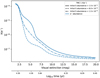 |
Fig. 1 Gas ionization fraction, X(e−), as a function of the visual extinction assuming different values of the initial sulfur elemental abundance in TMC 1. Calculations were performed using the gas-grain chemical code nautilus (Ruaud et al. 2016), with the physical structure and the updated chemical network described in Navarro-Almaida et al. (2020). |
2 CS chemical network
CS is among the most abundant gas phase S-bearing molecules in dark clouds. It is easily observable with several transitions in the millimeter wavelength range, and has a simple rotational spectrum with well-known collisional coefficients (Denis-Alpizar et al. 2018; Lique et al. 2006). Therefore, it has been largely used as a density and column density tracer in the interstellar medium in our Galaxy and external galaxies (see, e.g., Snell et al. 1984; Lapinov et al. 1998; Kim et al. 2020; Martín et al. 2005; Bayet et al. 2009; Kelly et al. 2015). Moreover, CS is the only S-bearing molecule routinely detected in protoplanetary disks and is therefore the main tracer of sulfur abundance in the primordial material to form planets (Agúndez et al. 2018; Le Gal et al. 2019). An understanding of CS chemistry is essential for correct interpretation of the observationsfrom all astrophysical environments. Unfortunately, chemical models do a poor job at accounting for these observations, usually predicting CS abundances much larger than those observed (Gratier et al. 2016; Vidal et al. 2017).
The chemistry of CS in interstellar clouds is closely correlated with that of HCS+ and involves reactions that have never been studied experimentally, leading to large uncertainties. For very young molecular clouds, where the ionization fraction from the diffuse period is still very large, sulfur is essentially in atomic ionized form and controls the chemistry of sulfur (e.g., Goicoechea et al. 2006). CS is then produced essentially from the electronic dissociative recombination (DR) of HCS+, HCS+ being produced bythe S+ + CH2 and CS+ + H2 reactions, and CS+ being produced by the ion-neutral reactions S+ + CH and S+ + C2. For the more advanced stages of dense clouds, which probably more closely correspond to the clouds observed in the GEMS project, the ionic fraction is much lower and the sulfur is mainly in neutral atomic form (the reactions of ionized atomic sulfur are not negligible but play a secondary role). Under these conditions, although the DR of HCS+ still produces CS, HCS+ is also mostly formed from CS (either directly by the CS + H reaction, or indirectly by CS + H+ → H + CS+ followed by CS+ + H2 → HCS+ + H) and not from S+ reactions. In that case, CS is produced by neutral reactions, mainly S + CH and S + C2, with secondary contributions by H + HCS, S + CH2, and C + SO. The overestimation of CS in the models versus the observations could come from an underestimation of the rates of consumption reactions (mainly CS + H+ and CS + H
 ). However, this seems unlikely because even if there are no measurements, the rates used are those resulting from the capture theory and thus close to the maximum theoretical rates. The CS overestimation could also come from overestimation of the production rates from neutral reactions such as S + CH and S + C2, or from missing consumption reactions of CS. For the latter case, Vidal et al. (2017) suggested that a high rate for the reaction of CS with the abundant atomic oxygen, O + CS, will decrease the overproduction of CS without heavily affecting the abundance of the S-bearing molecules, except for the chemically related HCS+. This possibility motivated the present study to better quantify the O + CS reaction rate.
Chemical models use the CS + O reaction rate constants measured by Lilenfeld & Richardson (1977) in the 150–300 K interval considerably higher than the typical Tk ~10 K of dark clouds, which are then extrapolated to low temperatures using the Arrhenius expression. The extrapolation to lower temperatures is always questionable and experimental measurement and/or theoretical calculations are needed to confirm these values. González et al. (1996) ran theoretical simulations by calculating the potential energy surface (PES) for the ground and first excited states and obtained reaction rate constants under several transition state theory (TST) approaches. However, the values found by these latter authors at 150−300 K were considerably lower than those seen in experimental measurements, casting doubts about the accuracy of the calculated rates. It is therefore necessary to improve the theoretical simulations to predict reasonable reaction rates at the lower temperatures prevailing inthe interstellar medium (ISM).
This study is devoted to the theoretical determination of the CS+O reaction rate. The ab initio calculations performed to produce the lower potential energy surfaces (PESs) are described in Sect. 3. These PESs are then used to study the reaction dynamics, using several methods (classical, quantum, and semiclassical) to derive the reactionrates. Finally, we test the role of the new reaction rates on realistic chemical models of cold dark clouds.
3 Potential energy surfaces
Calculation of the PES is a mandatory step for any dynamical study of a chemical reaction. The reaction
 (1)
(1)
involves open-shell atoms in reactants and products, presenting three degenerate electronic states at long distances (neglecting spin-orbit), correlating to P states of the oxygen or sulfur atoms. At long distances, the energies of these three states are dominated by the dipole-quadrupole interactions (Buckingham 1967). However, at short distances there are excited electronic states correlating to 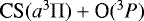 (González et al. 1996), which cross with the lower electronic manifold, giving rise to the formation of the
  products. These crossings give rise to small barriers whose height strongly depends on the electronic basis and the method chosen to describe the electronic correlation, as noted by González et al. (1996).
In this work accurate ab initio calculations are performed using the internally contracted multi-reference configuration interaction (ic-MRCI) method (Werner & Knowles 1988a,b) including the Davidson correction (icMRCI+Q) (Davidson 1975). In these calculations, the molecular orbitals are optimized using a state-averaged complete active space self-consistent field (SA-CASSCF) method, with an active space of 14 orbitals (11 and 3 of a′ and a″ symmetry, respectively). One 3A′ and two 3A″ electronic states are calculated and simultaneously optimized. In all these calculations the aug-cc-pVTZ basis set is used (Dunning 1989). For the ic-MRCI calculations, seven orbitals are kept doubly occupied, giving rise to ≈ 30 × 106 (6500 × 106) contracted (uncontracted) configurations. All ab initio calculations were performed with the MOLPRO suite of programs (Werner et al. 2012).
The analytical representation of the adiabatic PESs is done in three parts:
1. For short to intermediate distances, a three-dimensional cubic spline method is used with the DB3INK/DB3VAL subroutines based on the method of de Boor (1978) and distributed by GAMS (Boisvert 2015). A dense grid is calculated, composed of 20 × 14 × 19 points in the intervals defined in bond coordinates as: RCO ([0.9, 10] Å), RCS ([1, 7] Å), and ΘOCS ([0, π]), respectively.
2. At long distances (RCO > 8 Å), dipole-quadrupole long-range interactions are considered using the expressions defined by Zeimen et al. (2003) in reactant Jacobi coordinates. The V(RCS) obtained at RCO = 100 Å is fitted using the diatomic terms of Aguado & Paniagua (1992). The CS electric dipole is fitted as a function of the RCS distance, and the O(3P) quadrupole is calculated as energy derivatives using different homogeneous electric fields (Werner et al. 2012). The long-range behavior is checked by doing ic-MRCI calculations for distances R longer than 10 Å, with R being the distance between the CS center of mass and the oxygen atom.
3. In order to guarantee a continuous behavior between the previous two regions, points calculated with the long-range expression are added at RCO = 7, 8, and 9 Å, and a damping function among the two regions is centered at 5 Å.
The minimum energy path for the reaction is shown in Fig. 2 for the three adiabatic states (1 3 A′ and 2 3 A″). The reaction is exothermic by ≈3.9 eV, in agreement with the value of 3.93 eV reported by González et al. (1996). When zero-point energy (ZPE) is taken into account, theexothermicity reduces to 3.59 eV in rather good agreement with the experimental value of 3.64 eV (Lilenfeld & Richardson 1977). The energy barriers obtained in this work are 0.043, 0.058, and 0.888 eV for the 13 A’, 13 A”, and 23 A″ states, respectively. These values are lower than those obtained by González et al. (1996), probably because the electronic correlation introduced by ic-MRCI is higher than the PUMP4 method.
The main features of the present PESs are very similar to those discussed by González et al. (1996), represented in the contour plots shown in Fig. 3. The reaction barriers are located in the entrance channel, at nearly the equilibrium distance of CS, and at RCO ≈ 2.25 Å for the ground electronic state. In addition, the angular cone of acceptance is also reduced as R distance becomes closer: the saddle point is located at OCS angle, ΘOCS ≈ 120°, and the interval is reduced to [80°, 160°]. According to the Polanyi rules, the early barrier suggests that translational energy will enhance the reactivity. The reduction of the angular cone of acceptance is expected to introduce some restrictions, as discussed below in the reaction dynamics section.
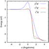 |
Fig. 2 Three lower adiabatic potential energy surfaces as a function of the intrinsic reaction coordinate (IRC) for the |

4 Reaction dynamics
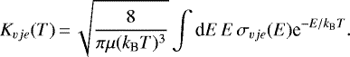
The thermal reaction rate can be defined as
 (2)
(2)
where the sum is over all vibrational, rotational, and electronic states of the reactants, CS(X1Σ+, v j) + O(3P), of energy Evje. Here, Kvje(T) are the initial state selected rate constants, which correspond to the Boltzmann average over the translational energy of the reaction cross-section,
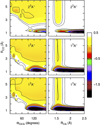 |
Fig. 3 Contour plots of the PES for the three electronic states obtained at the equilibrium RCS = 1.535 Å as a function of RCO and the OCSangle (left panels) and at an OCS angle of 120° as a functionof RCO and RCS distances. Energies are in eV, and the contour lines are at 0, 0.5, and 1 eV. |
 (3)
(3)
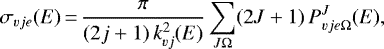
The cross-section is obtained under the partial wave summation over the total angular momentum, J, as
 (4)
(4)
where  (with μ being the CS + O reduced mass), Ω is the helicity, that is, the projection of J and j angular momenta on the z-axis of the body-fixed frame, and
  is the reaction probability for a particular initial state of the reactants, which depends on collision energy E. This quantity can be calculated with different methods: exact and approximate, quantum and classical. Below we start by determining the accuracy of each of them for J = 0.
The reaction is very exothermic, but it presents a reaction barrier. It can be assumed that all the flux that passes over this barrier yields products, considerably reducing the computational effort. This can be done using the quantum capture approach (Clary & Henshaw 1987), in which the time-independent close coupled equations (TICCEs) are solved in the entrance channel, similarly to what it is done in inelastic collisions, but subject to capture conditions, that is, to outgoing complex conditions at R < Rc for those channels for which E > VvjeΩ(Rc), with Rc = 2Å being the capture distance. Thus the TICCEs are integrated from R = 2 Å to 30 Å in the rovibrational states composed of CS(v = 0,1,2) and 50 rotational states for total angular momentum J = 0. This is done separately for each electronic state, 13A′ and 13A″ using the ZTICC code Gomez-Carrasco-et al. (in prep.). The capture probabilities are compared with quantum wave packet (WP) results in Fig. 4. These calculations were performed with the MADWAVE3 code (Zanchet et al. 2009) and the parameters used are listed in Table 1. The WP method is considered numerically exact, but as discussed below, it is very computationally demanding.
Clearly the quantum capture (QC) method overestimates the reaction probability. Near the reaction threshold, the QC and WP results are in rather good agreement, showing a common threshold at 0.04 and 0.06 eV for 13 A′ and 13 A″, respectively. However, above the threshold energy, the QC method gives a much larger reaction probability than the WP method. This is clear evidence that not all the flux arriving at distances R shorter than Rc go on to form CO + S products, and this situation increases with increasing collision energy.
As the reaction involves rather heavy atoms, it may be expected that quantum effects do not play an important role. The quasi-classical trajectory (QCT) method is then an interesting alternative to simplify the computationally demanding quantum WP calculations. The comparison for J = 0 in Fig. 4 reveals rather good agreement, except at the threshold. The QCT method is not able to describe the first peaks appearing in the WP reaction probabilities, which can be attributed to tunneling.
To better quantify the adequacy of the QCT method to describe this reaction, we calculated the total cross-section with the QCT and WP methods. In order to limit the highly demanding WP calculations for high J, we performed the centrifugal sudden approximation (CSA); (Pack 1974; McGuire & Kouri 1974), in which only one helicity Ω is included. Also, we calculated the reaction probability for J = 0, 50, 100, 150 and 180, and the reaction probabilities for the remaining Js are obtained using an interpolation based on the J-shifting approximation (Aguado et al. 1997; Zanchet et al. 2013). The comparison between the WP-CS and QCT calculations is shown in Fig. 5, and they show reasonably good agreement below 0.2 eV. However, for higher energies, the QCT cross-sections are in general higher than the WP-CS ones, and the differences are larger for 13 A′ than for 13 A″. At these higher energies one would expect better agreement between classical and quantum methods, similar to that obtained for J = 0. The larger difference can be attributed to the CS approximation made to obtain the cross-section in the case of the quantum WP-CS method. In order to check this, for the 13A′ state and J = 50, 100, and 150 we included more helicities on the reaction probabilities, Ω = 0,1, 2, 3, 4, and 5. These new calculations, labeled ‘WP’ in Fig. 5, are larger than the WP-CS calculations, and very close to the QCT calculations up to 0.3 eV. Above this energy, more helicities Ω are needed to converge the reaction probabilities of J > 100. However, these calculations are extremely demanding.
In Fig. 5 the probability arising for a Boltzmann distribution at 300 K is also displayed, showing that only collision energy below 0.12 eV contributes for temperatures below 300 K. Below 0.12 eV, QCT results are lower than the quantum wave packet values. This indicates that it is important to include quantum effects near the threshold. WP methods require individual calculations for each initial state, and many rotational states have to be considered (which contribute significantly below 0.12 eV) because of the low rotational constant of CS. This makes the use of the WP method in evaluating the thermal rate constants for this reaction very computationally demanding, and some alternative method should be used. The QC results for energies below 0.07 eV are in very good agreement with the exact WP calculations. However, QC results clearly overestimate the reaction cross-section for higher energies. Nevertheless, the Boltzmann energy distribution corresponds to collision energies below 0.07 eV for temperatures below 150 K and therefore the QC results can be considered to be nearly exact in this low temperature range.
Ring polymer molecular dynamics (RPMD) is a semiclassical method based on path integral methods that include quantum effects such as zero-point energy and tunneling proposed by Craig & Manolopoulos (2004). RPMD has been successfully applied to calculate reaction rate constants (Craig & Manolopoulos 2005a,b; Suleimanov et al. 2011) as recently reviewed by Suleimanov et al. (2016). Here we apply a direct version of this method recently applied to reactions of polyatomic molecules at low temperature(Suleimanov et al. 2018; del Mazo-Sevillano et al. 2019; Bulut et al. 2019) and implemented in the code dRPMD.
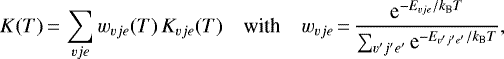
RPMD, QCT, and QC results are compared in Fig. 6 for the 1 3 A′ and 1 3 A″ electronic states. The QCT calculations consist of more than 105 trajectories per temperature (for low temperatures, more than 106 trajectories were needed to get convergence). RPMD results are based on 104 trajectories using a variable number of beads (64 for 300 K, 128 for 150 K, etc.). RPMD rate constants are always about ten times larger than the QCT ones. This is explained by the difference found in the cross-section obtained with quantum WP and QCT methods at energies below 0.12 eV. RPMD includes quantum effects and the results show that it is more accurate than the QCT. It is important to stress here that, according to QC calculations, the reaction probability at low energies increases with the initial rotational state of the CS reagent. The QCT and RPMD rate calculations include this effect by considering the rotational temperature, and this produces an amplification of the difference between QCT and RPMD rate constants. In both cases, many trajectories have been run for temperatures below 100 K, but no reactive ones were found. This indicates that the reaction rate constant below 100 K is very small. The QC results at 150 K are very close to the RPMD rate constant. For 200 K, however, QC results are considerably larger. This result is expected as QC overestimates the reaction probabilities above 0.07 eV. However, for temperatures below 150 K it is expected to be a rather good upper limit of the reaction rate constant.
The thermal rate constant is finally obtained by an average over the spin-orbit electronic states of O(3 P) as
 (5)
(5)
where an adiabatic approximation has been made for the spin-orbit states, and  . The results are compared with the experimental results of Lilenfeld & Richardson (1977) in Fig. 7. The results of the calculations presented here are close to the experimental values for T = 150–200 K, becoming a factor of between two and three smaller at 300 K. According to the fit to the Arrhenius law shown in Fig. 7 the activation energy is ≈0.065 eV, while the potential energy barriers obtained here are lower, namely 0.043 and 0.058 for the 13 A′ and 13 A″ states, respectively. Furthermore, the rate constant obtained for the 1 3A′ state alone is very close to the experimental value, changing the slope of the rate constant versus temperature. The disagreement at 300 K is attributed to inaccuracies of the 1,23A″ excited electronic states. Also, as RPMD includes quantum effects such as tunneling and zero-point energy effects, we may conclude that the rate constant decreases with temperature, following an Arrhenius law. This Arrehenius-like behavior is found in the QC results below 150 K, confirming the behavior in the fitted rate constant to the experimental values (note that the rate constant for the 13A″ is lower). Therefore, we may conclude that at the temperatures relevant in dense molecular clouds, Tk ~ 10 K, the CS + O reaction rate constant is negligible, below 10−15 cm3 s−1.
Parameters used in the wave packet calculations in reactant Jacobi coordinates.
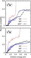 |
Fig. 4 CS+O → CO + S reaction probabilities vs. collision energy for J = 0 in the 1 3A′ and 1 3 A″ electronic states using three different methods described in the text: the QC, the WP, and the QCT methods. |
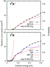 |
Fig. 5 CS + O → CO + S reaction cross-section (in Bohr2) vs. collision energy for 1 3A′ and 1 3 A″ electronic states using the quantum wave packet within the CS approach (WP-CSA) and the QCT methods. ‘QC’ labels the results obtained with the QC method. The energy distribution of a Boltzmann distribution for a temperature of 300 K is also shown in green. For the 1 3 A′, WP labels the wave-packet calculations performed including Ω = 0, 1, 2, 3, 4 and 5. |
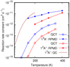 |
Fig. 6 CS+O → CO + S reaction rate constants obtained with RPMD (full circles) and QCT (open squares) for the 13 A′ (blue) and 13A″ (red) electronic states. |
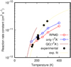 |
Fig. 7 Comparison of the calculated thermal rate constant for the CS+O → CO + S reaction including spin-orbit splitting and the experimental measurements of Lilenfeld & Richardson (1977). The rate constant obtained for 13A′ is included for discussion. The experimental results are fit to k = Ae−C∕T, with A = 2.6 10−10 cm3 s−1 and C = 757.7 K = 0.065 eV. |
5 Astrophysical implications
Here we present a detailed theoretical study of the CS+O reaction, confirming the experimental data obtained at 150–400 K, and after a careful analysis at lower temperatures we find that the rate constant at 10 K is negligible, below 10−15 cm3 s−1. Given the low value of the rate constant of the CS + O reaction at low temperature, this reaction does not seem to be able to explain the calculated overabundance of CS given by dense cloud models. A CS + O reaction rate close to 1 × 10⁻¹⁰ cm3 s−1 at 10 K, five orders of magnitude higher than our limit, would be needed to account for the observed CS abundances if no ad hoc depletion of sulfur is assumed. In addition to the O + CS reaction, the chemical network for the destruction reactions of CS seems to us complete and relatively precise. The overestimation of CS does not seem to be due to an underestimation of the CS destruction reactions. Another hypothesis for the cause of this overestimation, previously put forward in the section above (CS chemical network), could be an overestimation of the CS production reactions. For a typical chemical evolution of the clouds corresponding to the observations, CS is mainly produced by neutral reactions, that is, mainly S + CH and S + C2. The rates for these two reactions in the model are close to those given by the capture theory, which may overestimate the value. A decrease in these rates would lead to a decrease in the production of CS because, despite their importance, the fluxes of these reactions are smaller than the fluxes of the S + H , S + OH, S + CH3 reactions considering the CH, C2, H
 , OH, and CH3 abundances given by the model (and for some of them by the observations) considering the physical conditions of the studied dark clouds. To our knowledge, there are no experimental data for or theoretical studies of the S + CH and S + C2 reactions. Indeed, there is very little information on S + radical reactions in general. Flores et al. (2001) performed a theoretical study of the S + C2H reaction leading to a very high rate constant at low temperature, similar to the O + C2 H one (Georgievskii & Klippenstein 2011). Therefore, as the O + CH reaction is rapid at room temperature characteristic of a barrierless reaction (Messing et al. 1980), we may expect similar behavior for the S + CH reaction and a high rate constant at low temperature. An overestimation of the S + CH and S + C2 reactions required to reproduce the CS abundances by more than a factor of ten seems unlikely. Nevertheless, it is clear that theoretical and experimental studies are needed to better characterize S + radical reactions.
An additional problem comes from the fact that if the abundance of CS decreases, the abundance of HCS+ would also decrease in typical dense clouds, because in this case HCS+ is mainly produced from CS. Furthermore, as the measured abundances of HCS+ are significantly higher than the modeled abundances, the decrease of CS will accentuate the disagreement. Either there is an unknown direct production (not from CS) of HCS+ or the destruction of HCS+ is overestimated. As the DR of HCS+ is by far the main loss of HCS+, a smaller value of the rate constant for this DR will increase the HCS+ abundance. This DR has been experimentally studied by Montaigne et al. (2005) and there are no specific reasons to question this value. Nevertheless, there is only an experimental value and it should be noted that the DR of HCNH+ (Adams et al. 1991; Semaniak et al. 2001; McLain & Adams 2009) and N2 H+ (Shapko et al. 2020) vary greatly from one measurement to another. New experimental measurements of the DR of HCS+ would be desirable to confirm the currently used value.
In order to evaluate the impact of our calculated CS + O reaction rate, we modeled the GEMS data along the dense clouds TMC 1-C, TMC 1-CP, and TMC 1-NH3. These data were recently presented and modeled by Fuente et al. (2019) and Navarro-Almaida et al. (2020). Here, we resumed this modeling focusing on CO, CS, and HCS+. For this modeling we used the updated network from Vidal et al. (2017) and the same temperatures, densities, incident UV flux, and visual extinction (AV) of each observed region as those used by Navarro-Almaida et al. (2020). For the cosmic-ray molecular hydrogen ionization rate,  , we use the fixed value equal to 10−16s−1 as determined by Fuente et al. (2019). The results of these simulations are presented in Figs. 8–13 for CS, HCS+, and CO. In these figures, the colored boxes represent the period of time in which model predictions agree with observed abundance ratios at each position. An uncertainty of a factor of two is assumed for the observed abundances, which translates into an uncertainty of a factor of four in the molecular abundance ratios. The abundance of CO makes it possible to accurately constrain the maximum age of the clouds since CO is rapidly depleted under the physicalconditions of these clouds. The CS profile is flat and the only way to obtain a good agreement between theobservations and the model is to strongly deplete the sulfur elemental abundance (by a factor of 20 in the curves shown in Figs. 8–13). In this case, the agreement for CS and HCS+ can only be considered as ‘satisfactory’, as HCS+ is underestimated for TMC 1-CP, while CO is also fairly well modeled. However, with such a sulfur depletion factor, the H2 S abundance would remain underestimated by a factor of more than ten (see Navarro-Almaida et al. 2020), thus challenging our comprehension of the sulfur chemistry.
A crucial point in the modeling of sulfur compounds, in addition to the sulfur depletion factor, is the specific dependency of their abundances on the cosmic-ray ionization rate (see e.g., Fuente et al. 2016). It is known that the cosmic ray flux decreases with AV following a law that is dependent on the local conditions (Padovani et al. 2009, 2013, 2018; Ivlev et al. 2018). Thus far, we have used a fixed value of  in our simulations. One may postulate that the disagreement between chemical predictions and observations is due to the adopted fixed value for
  . In order to evaluate this effect, we repeated the simulations assuming
  to change with AV. In particular we assumed a different value of
  for each AV following the fit shown in Fig. 6 of Neufeld & Wolfire (2017).
 (6)
(6)
This expression gives values of  ~ 10−17 s−1 for an AV of 13 mag and ~ 4 × 10⁻¹⁷ s−1 for an AV of 5 mag. These values are significantly lower than the value previously adopted (
 = 10−16 s−1). Figures 11, 12, and 13 show model predictions using the new values of
  . Interestingly, the value of
  has a great impact on the CS and HCS+ abundances, but its impact is negligible for CO. With these new values, the CS profiles are much more stepped, with a shape similar to that of CO. In this case, one can always find a cloud age that allows reproduction of CS regardless of the sulfur depletion factor. However, the obtained ages are only compatible with CO abundances when we assume a low value for the elemental sulfur abundance. More specifically, the ages required to account for the observed CS abundances are too large for CO, which would be strongly depleted on the grain surfaces unless we assume that sulfur elemental abundance is depleted by a factor of ~20. Figures 8, 9, and 10 show the comparison between models and observations assuming that the elemental sulfur abundance is depleted by a factor 20 with the observations. The agreement is good for CS but in this case it is more difficult to reproduce the abundance of HCS+ for ages where CS is reproduced. In addition, we still do not reproduce the H2 S abundance (Navarro-Almaida et al. 2020). We therefore conclude that decreasing the cosmic ray flux with AV does not help to find a better agreement between chemical models and observations.
Our study on the rate of the O + CS reaction removes one of the hypotheses for the overestimation of CS in the models versus the previous observations. The new analysis of GEMS observations using an updated chemical network shows the importance of the cosmic-ray ionization rate on the predicted abundances of sulfur-bearing species in cold dark clouds. However, we are not able to reproduce observations by decreasing  with the visual extinction. Further observational and theoretical research is needed. From the observational point of view, it would be desirable to complete the molecular database with important sulfur-bearing species other than CS, HCS+, and H2 S, in particular C2S, C3 S, OCS, and H2CS to better constrain the value of the cosmic-ray ionization rate and its coupling with the sulfur depletion factor. From the theoretical point of view, there is still room for significant improvement. Despite recent reviews on the chemistry of sulfur (Fuente et al. 2017, 2019; Vidal et al. 2017; Laas & Caselli 2019; Navarro-Almaida et al. 2020; Shingledecker et al. 2020), the rates and branching ratios of sulfur chemistry reactions are too poorly known, which prevents the models from being really predictive. A substantial theoretical and experimental effort on the rates of neutral atomic sulfur reactions, on the branching ratios of S+ reactions and on HCS+ DR rate is needed if we hope to better understand the chemistry of sulfur in the interstellar medium.
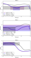 |
Fig. 8 Predicted abundances of gas-phase CS, HCS+, and CO withrespect to H2 as a function of time. The curves correspond to the different physical conditions observed in the TMC1-C source with |

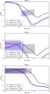 |
Fig. 11 Same as in Fig. 8 but with |


6 Conclusions
The CS+O reaction has been proposed as a relevant CS destruction mechanism at low temperatures. Its reaction rate has been experimentally measured at temperatures of 150−400 K, but the extrapolation to lower temperatures is uncertain. In this study, we calculated the CS+O reaction rate at temperatures <150 K which are prevailing in cold dark clouds. We performed ab initio calculations to produce the lower potential energy surfaces (PESs) of the CS+O system. These PESs are used to study the reaction dynamics, using several classical, quantum, and semiclassical methods to eventually calculate the CS+O thermal reaction rates. In order to check the accuracy of our calculations, we compared the results with those obtained in the laboratory over the T ~ 150−400 K range. We present a detailed theoretical study of the CS + O reaction, the results of which are in agreement with experimental data, verifying the reliability of our approach. After careful analysis at lower temperatures we find that the rate constant at 10 K is negligible, below 10−15 cm3 s−1, consistent with the extrapolation of experimental data using the Arrhenius expression.
We modeled observations of CS and HCS+ using an updated chemical network. We obtain a good fit of the CS, HCS+, and SO abundances assuming a sulfur depletion by a factor of 20 and different chemical ages for each position within the cloud. Still, the H2 S abundance would remain underestimated by a factor of more than ten unless we assume no sulfur depletion (S/H = 1.5 × 10⁻⁵). We also investigated the effect of the decrease of  with AV on the abundances of S-bearing species. Still, we need to adopt a sulfur depletion by a factor of 20 if we want to fit the abundances of CO, CS, and HCS+ using the same chemical age. This high depletion would lead to underestimation of the H2 S abundance. Therefore, further theoretical and observational research is needed to understand the sulfur chemistry. In spite of recent efforts to complete and update sulfur chemistry (Fuente et al. 2017, 2019; Vidal et al. 2017; Laas & Caselli 2019; Navarro-Almaida et al. 2020; Shingledecker et al. 2020), there are still many uncertainties in the chemical network. A substantial theoretical and experimental effort on the rates of neutral atomic sulfur reactions, on the branching ratios of S+ reactions, and on the HCS+ DR rate is needed if we hope to better understand the chemistry of sulfur in the interstellar medium. The observation of a wide inventory of S-bearing species is also necessary to better constrain the physical parameters, in particular the cosmic-ray ionization rate for H2 and its variation along the cloud.
Acknowledgements
The research leading to these results has received funding from MICIU (Spain) under grants FIS2017-83473-C2, AYA2016-75066-C2-2-P, ESP2017-86582-C4-1-R, AYA2017-85111-P, PID2019-105552RB-C41 and PID2019-106235GB-I00. N.B. acknowledges the computing facilities by TUBITAK-TRUBA, and O.R. and A.A. acknowledge computing time at Finisterre (CESGA) and Marenostrum (BSC) under RES computational grants ACCT-2019-3-0004 and AECT-2020-1-0003. SPTM acknowledges the European Union’s Horizon 2020 research and innovation program for funding support under agreement No 639450 (PROMISE).
References
- Adams, N. G., Herd, C. R., Geoghegan, M., et al. 1991, J. Chem. Phys., 94, 4852 [NASA ADS] [CrossRef] [Google Scholar]
- Aguado, A., & Paniagua, M. 1992, J. Chem. Phys., 96, 1265 [NASA ADS] [CrossRef] [Google Scholar]
- Aguado, A., Paniagua, M., Lara, M., & Roncero, O. 1997, J. Chem. Phys., 106, 1013 [CrossRef] [Google Scholar]
- Agúndez, M., & Wakelam, V. 2013, Chem. Rev., 113, 8710 [Google Scholar]
- Agúndez, M., Roueff, E., Le Petit, F., & Le Bourlot, J. 2018, A&A, 616, A19 [NASA ADS] [CrossRef] [EDP Sciences] [Google Scholar]
- Anderson, D. E., Bergin, E. A., Maret, S., & Wakelam, V. 2013, ApJ, 779, 141 [NASA ADS] [CrossRef] [Google Scholar]
- Bayet, E., Aladro, R., Martín, S., Viti, S., & Martín-Pintado, J. 2009, ApJ, 707, 126 [NASA ADS] [CrossRef] [Google Scholar]
- Boisvert, R. F. 2015, http://gams.nist.gov/ [Google Scholar]
- Buckingham, A. D. 1967, Adv. Chem. Phys., 12, 107 [CrossRef] [Google Scholar]
- Bulut, N., Aguado, A., Sanz-Sanz, C., & Roncero, O. 2019, J. Phys. Chem. A, 123, 8766 [CrossRef] [Google Scholar]
- Calmonte, U., Altwegg, K., Balsiger, H., et al. 2016, MNRAS, 462, S253 [CrossRef] [Google Scholar]
- Caselli, P., Walmsley, C. M., Zucconi, A., et al. 2002, ApJ, 565, 344 [Google Scholar]
- Clary, D. C., & Henshaw, J. P. 1987, Faraday Discuss. Chem. Soc., 84, 333 [CrossRef] [Google Scholar]
- Craig, I. R., & Manolopoulos, D. E. 2004, J. Chem. Phys., 121, 3368 [CrossRef] [Google Scholar]
- Craig, I. R., & Manolopoulos, D. E. 2005a, J. Chem. Phys., 122, 084106 [CrossRef] [Google Scholar]
- Craig, I. R., & Manolopoulos, D. E. 2005b, J. Chem. Phys., 123, 034102 [CrossRef] [Google Scholar]
- Davidson, E. R. 1975, J. Comp. Phys., 17, 87 [NASA ADS] [CrossRef] [MathSciNet] [Google Scholar]
- de Boor, C. 1978, A Practical Guide to Splines (New York: Springer-Verlag) [Google Scholar]
- del Mazo-Sevillano, P., Aguado, A., Jiménez, E., Suleimanov, Y. V., & Roncero, O. 2019, J. Phys. Chem. Lett., 10, 1900 [CrossRef] [Google Scholar]
- Denis-Alpizar, O., Stoecklin, T., Guilloteau, S., & Dutrey, A. 2018, MNRAS, 478, 1811 [NASA ADS] [CrossRef] [Google Scholar]
- Dunning, T. H. 1989, J. Chem. Phys., 90, 1007 [NASA ADS] [CrossRef] [Google Scholar]
- Esplugues, G. B., Viti, S., Goicoechea, J. R., & Cernicharo, J. 2014, A&A, 567, A95 [NASA ADS] [CrossRef] [EDP Sciences] [Google Scholar]
- Flores, J. R., Estévez, C. M., Carballeira, L., & Juste, I. P. 2001, J. Phys. Chem. A, 105, 4716 [CrossRef] [Google Scholar]
- Fuente, A., Cernicharo, J., Roueff, E., et al. 2016, A&A, 593, A94 [NASA ADS] [CrossRef] [EDP Sciences] [Google Scholar]
- Fuente, A., Gerin, M., Pety, J., et al. 2017, A&A, 606, L3 [NASA ADS] [CrossRef] [EDP Sciences] [Google Scholar]
- Fuente, A., Navarro, D. G., Caselli, P., et al. 2019, A&A, 624, A105 [NASA ADS] [CrossRef] [EDP Sciences] [Google Scholar]
- Georgievskii, Y., & Klippenstein, S. J. 2011, Proc. IAU Symp., 280, 372 [CrossRef] [Google Scholar]
- Goicoechea, J. R., Pety, J., Gerin, M., et al. 2006, A&A, 456, 565 [NASA ADS] [CrossRef] [EDP Sciences] [Google Scholar]
- González, M., Hijazo, H., Novoa, J. J., & R., S. 1996, J. Chem. Phys., 105, 10999 [CrossRef] [Google Scholar]
- Gratier, P., Majumdar, L., Ohishi, M., et al. 2016, ApJS, 225, 25 [NASA ADS] [CrossRef] [Google Scholar]
- Holdship, J., Viti, S., Jimenez-Serra, I., et al. 2016, MNRAS, 463, 802 [NASA ADS] [CrossRef] [Google Scholar]
- Indriolo, N., & McCall, B. J. 2012, ApJ, 745, 91 [NASA ADS] [CrossRef] [Google Scholar]
- Ivlev, A. V., Dogiel, V. A., Chernyshov, D. O., et al. 2018, ApJ, 855, 23 [NASA ADS] [CrossRef] [Google Scholar]
- Jiménez-Escobar, A., & Muñoz Caro, G. M. 2011, A&A, 536, A91 [NASA ADS] [CrossRef] [EDP Sciences] [Google Scholar]
- Kelly, G., Viti, S., Bayet, E., Aladro, R., & Yates, J. 2015, A&A, 578, A70 [CrossRef] [EDP Sciences] [Google Scholar]
- Kim, S., Lee, C. W., Gopinathan, M., et al. 2020, ApJ, 891, 169 [CrossRef] [Google Scholar]
- Laas, J. C., & Caselli, P. 2019, A&A, 624, A108 [CrossRef] [EDP Sciences] [Google Scholar]
- Lapinov, A. V., Schilke, P., Juvela, M., & Zinchenko, I. I. 1998, A&A, 336, 1007 [NASA ADS] [Google Scholar]
- Le Gal, R., Öberg, K. I., Loomis, R. A., Pegues, J., & Bergner, J. B. 2019, ApJ, 876, 72 [NASA ADS] [CrossRef] [Google Scholar]
- Lilenfeld, H. V., & Richardson, R. J. 1977, J. Chem. Phys., 67, 3991 [CrossRef] [Google Scholar]
- Lique, F., Spielfiedel, A., & Cernicharo, J. 2006, A&A, 451, 1125 [NASA ADS] [CrossRef] [EDP Sciences] [Google Scholar]
- Martín, S., Martín-Pintado, J., Mauersberger, R., Henkel, C., & García-Burillo, S. 2005, ApJ, 620, 210 [NASA ADS] [CrossRef] [Google Scholar]
- McGuire, P., & Kouri, D. 1974, J. Chem. Phys., 60, 2488 [NASA ADS] [CrossRef] [Google Scholar]
- McKee, C. F. 1989, ApJ, 345, 782 [NASA ADS] [CrossRef] [Google Scholar]
- McLain, J. L., & Adams, N. G. 2009, Planet. Space Sci., 57, 1642 [CrossRef] [Google Scholar]
- Messing, I., Carrington, T., Filseth, S. V., & Sadowski, C. M. 1980, Chem. Phys. Lett., 74, 56 [CrossRef] [Google Scholar]
- Minissale, M., Dulieu, F., Cazaux, S., & Hocuk, S. 2016, A&A, 585, A24 [NASA ADS] [CrossRef] [EDP Sciences] [Google Scholar]
- Montaigne, H., Geppert, W. D., Semaniak, J., et al. 2005, ApJ, 631, 653 [NASA ADS] [CrossRef] [Google Scholar]
- Navarro-Almaida, D., Le Gal, R., Fuente, A., et al. 2020, A&A, 637, A39 [CrossRef] [EDP Sciences] [Google Scholar]
- Neufeld, D. A., & Wolfire, M. G. 2017, ApJ, 845, 163 [Google Scholar]
- Neufeld, D. A., Godard, B., Gerin, M., et al. 2015, A&A, 577, A49 [NASA ADS] [CrossRef] [EDP Sciences] [Google Scholar]
- Pack, R. T. 1974, J. Chem. Phys., 60, 633 [NASA ADS] [CrossRef] [Google Scholar]
- Padovani, M., Galli, D., & Glassgold, A. E. 2009, A&A, 501, 619 [NASA ADS] [CrossRef] [EDP Sciences] [Google Scholar]
- Padovani, M., Hennebelle, P., & Galli, D. 2013, A&A, 560, A114 [NASA ADS] [CrossRef] [EDP Sciences] [Google Scholar]
- Padovani, M., Ivlev, A. V., Galli, D., & Caselli, P. 2018, A&A, 614, A111 [NASA ADS] [CrossRef] [EDP Sciences] [Google Scholar]
- Ruaud, M., Wakelam, V., & Hersant, F. 2016, MNRAS, 459, 3756 [NASA ADS] [CrossRef] [Google Scholar]
- Ruffle, D. P., Hartquist, T. W., Caselli, P., & Williams, D. A. 1999, MNRAS, 306, 691 [NASA ADS] [CrossRef] [Google Scholar]
- Semaniak, J., Minaev, B. F., Derkatch, A. M., et al. 2001, ApJS, 135, 275 [NASA ADS] [CrossRef] [Google Scholar]
- Shapko, D., Dohnal, P., Kassayová, M., et al. 2020, J. Chem. Phys., 152, 024301 [CrossRef] [Google Scholar]
- Shingledecker, C. N., Lamberts, T., Laas, J. C., et al. 2020, ApJ, 52 [NASA ADS] [CrossRef] [Google Scholar]
- Snell, R. L., Mundy, L. G., Goldsmith, P. F., Evans, N. J., I., & Erickson, N. R. 1984, ApJ, 276, 625 [NASA ADS] [CrossRef] [Google Scholar]
- Suleimanov, Y. V., Collepardo-Guevara, R., & Manolopoulos, D. E. 2011, J. Chem. Phys., 134, 044131 [CrossRef] [Google Scholar]
- Suleimanov, Y. V., Aoiz, F. J., & Guo, H. 2016, J. Phys. Chem. A, 120, 8488 [CrossRef] [Google Scholar]
- Suleimanov, Y. V., Aguado, A., Gómez-Carrasco, S., & Roncero, O. 2018, J. Phys. Chem. Lett., 9, 2133 [CrossRef] [Google Scholar]
- Tieftrunk, A., Pineau des Forets, G., Schilke, P., & Walmsley, C. M. 1994, A&A, 289, 579 [Google Scholar]
- Vastel, C., Quénard, D., Le Gal, R., et al. 2018, MNRAS, 478, 5514 [NASA ADS] [CrossRef] [Google Scholar]
- Vidal, T. H. G., & Wakelam, V. 2018, MNRAS, 474, 5575 [NASA ADS] [CrossRef] [Google Scholar]
- Vidal, T. H. G., Loison, J.-C., Jaziri, A. Y., et al. 2017, MNRAS, 469, 435 [NASA ADS] [CrossRef] [Google Scholar]
- Wakelam, V., Ceccarelli, C., Castets, A., et al. 2005, A&A, 437, 149 [NASA ADS] [CrossRef] [EDP Sciences] [Google Scholar]
- Werner, H. J., & Knowles, P. J. 1988a, J. Chem. Phys., 89, 5803 [NASA ADS] [CrossRef] [Google Scholar]
- Werner, H. J., & Knowles, P. J. 1988b, Chem. Phys. Lett., 145, 514 [NASA ADS] [CrossRef] [Google Scholar]
- Werner, H.-J., Knowles, P. J., Knizia, G., Manby, F. R., & Schütz, M. 2012, WIRE Comput. Mol. Sci., 2, 242 [CrossRef] [Google Scholar]
- Zanchet, A., Roncero, O., González-Lezana, T., et al. 2009, J. Phys. Chem. A, 113, 14 488 [CrossRef] [PubMed] [Google Scholar]
- Zanchet, A., Godard, B., Bulut, N., et al. 2013, ApJ, 766, 80 [NASA ADS] [CrossRef] [Google Scholar]
- Zeimen, W. B., Klos, J., Groenenboom, G. C., & van der Avoird, A. 2003, J. Chem. Phys., 118, 7340 [CrossRef] [Google Scholar]
- Zhao, B., Caselli, P., Li, Z.-Y., et al. 2016, MNRAS, 460, 2050 [Google Scholar]
All Tables
All Figures
|
Fig. 1 Gas ionization fraction, X(e−), as a function of the visual extinction assuming different values of the initial sulfur elemental abundance in TMC 1. Calculations were performed using the gas-grain chemical code nautilus (Ruaud et al. 2016), with the physical structure and the updated chemical network described in Navarro-Almaida et al. (2020). |
| In the text | |
|
Fig. 2 Three lower adiabatic potential energy surfaces as a function of the intrinsic reaction coordinate (IRC) for the |
| In the text | |
|
Fig. 3 Contour plots of the PES for the three electronic states obtained at the equilibrium RCS = 1.535 Å as a function of RCO and the OCSangle (left panels) and at an OCS angle of 120° as a functionof RCO and RCS distances. Energies are in eV, and the contour lines are at 0, 0.5, and 1 eV. |
| In the text | |
|
Fig. 4 CS+O → CO + S reaction probabilities vs. collision energy for J = 0 in the 1 3A′ and 1 3 A″ electronic states using three different methods described in the text: the QC, the WP, and the QCT methods. |
| In the text | |
|
Fig. 5 CS + O → CO + S reaction cross-section (in Bohr2) vs. collision energy for 1 3A′ and 1 3 A″ electronic states using the quantum wave packet within the CS approach (WP-CSA) and the QCT methods. ‘QC’ labels the results obtained with the QC method. The energy distribution of a Boltzmann distribution for a temperature of 300 K is also shown in green. For the 1 3 A′, WP labels the wave-packet calculations performed including Ω = 0, 1, 2, 3, 4 and 5. |
| In the text | |
|
Fig. 6 CS+O → CO + S reaction rate constants obtained with RPMD (full circles) and QCT (open squares) for the 13 A′ (blue) and 13A″ (red) electronic states. |
| In the text | |
|
Fig. 7 Comparison of the calculated thermal rate constant for the CS+O → CO + S reaction including spin-orbit splitting and the experimental measurements of Lilenfeld & Richardson (1977). The rate constant obtained for 13A′ is included for discussion. The experimental results are fit to k = Ae−C∕T, with A = 2.6 10−10 cm3 s−1 and C = 757.7 K = 0.065 eV. |
| In the text | |
|
Fig. 8 Predicted abundances of gas-phase CS, HCS+, and CO withrespect to H2 as a function of time. The curves correspond to the different physical conditions observed in the TMC1-C source with |
| In the text | |
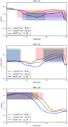 |
Fig. 9 Sameas Fig. 8 but for TMC1-CP. |
| In the text | |
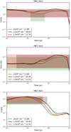 |
Fig. 10 Same as Fig. 8 but for TMC1-NH3. |
| In the text | |
|
Fig. 11 Same as in Fig. 8 but with |
| In the text | |
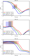 |
Fig. 12 Same as in Fig. 9, but with |
| In the text | |
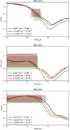 |
Fig. 13 Same as in Fig. 10 but with |
| In the text | |
Current usage metrics show cumulative count of Article Views (full-text article views including HTML views, PDF and ePub downloads, according to the available data) and Abstracts Views on Vision4Press platform.
Data correspond to usage on the plateform after 2015. The current usage metrics is available 48-96 hours after online publication and is updated daily on week days.
Initial download of the metrics may take a while.