| Issue |
A&A
Volume 651, July 2021
|
|
|---|---|---|
| Article Number | A43 | |
| Number of page(s) | 16 | |
| Section | Interstellar and circumstellar matter | |
| DOI | https://doi.org/10.1051/0004-6361/202039226 | |
| Published online | 09 July 2021 | |
Combined hydrodynamic and gas-grain chemical modeling of hot cores
I. One-dimensional simulations
1
Department of Chemistry, University of Virginia,
Charlottesville,
VA
29904-4319,
USA
2
Department of Astronomy, University of Virginia,
Charlottesville,
VA
22904-4325,
USA
e-mail: rgarrod@virginia.edu
Received:
21
August
2020
Accepted:
3
April
2021
Context. Gas-grain models have long been employed to simulate hot-core chemistry; however, these simulations have traditionally neglected to couple chemical evolution in tandem with a rigorous physical evolution of a source. This over-simplification particularly lacks an accurate treatment of temperature and spatial distribution, which are needed for realistic simulations of hot cores.
Aims. We aim to combine radiation hydrodynamics (RHD) with hot-core chemical kinetics in one dimension to produce a set of astrochemical models that evolve according to explicitly calculated temperature, density, and spatial profiles.
Methods. We solve radiation hydrodynamics for three mass-accretion-rate models using Athena++. We then simulate the chemistry using the hot-core chemical kinetic code MAGICKAL according to the physics derived from the RHD treatment.
Results. We find that as the mass-accretion rate decreases, the overall gas density of the source decreases. In particular, the gas density for the lowest mass-accretion rate is low enough to restrict the proper formation of many complex organic molecules. We also compare our chemical results in the form of calculated column densities to those of observations toward Sgr B2(N2). We find a generally good agreement for oxygen-bearing species, particularly for the two highest mass-accretion rates.
Conclusions. Although we introduce hot-core chemical modeling using a self-consistent physical treatment, the adoption of a two-dimensional model may better reproduce chemistry and physics toward real sources and thus achieve better chemical comparisons with observations.
Key words: astrochemistry / hydrodynamics / ISM: abundances / ISM: molecules / magnetohydrodynamics (MHD) / molecular processes
© ESO 2021
1 Introduction
Hot cores are high-mass star-forming regions with temperatures and gas densities in excess of 100 K and 107 cm−3, respectively. A notable feature of hot cores is their rich molecular line-emission in the millimeter to sub-millimeter range. A variety of complex organic molecules (COMs), including alcohols, aldehydes, esters, acids, and amines, have been detected in high abundances toward these objects (Herbst & van Dishoeck 2009; Garrod & Widicus Weaver 2013). Furthermore, high gas densities allow COM emission in hot cores to be well approximated by local thermodynamic equilibrium (LTE). In LTE, measured or modeled excitation temperatures represent local gas kinetic temperatures, which make COMs valuable tracers of the inner thermal structure of hot cores. The rich chemical complexity of these sources makes them compelling objects to study, and they offer an appropriate setting in which theories of COM formation and processing in the interstellar medium (ISM) can be tested and refined.
Hot-core chemistry has long been known to be associated with the formation and sublimation of dust-grain ice mantles (Millar et al. 1991; Charnley et al. 2005). Simple molecules, including water, carbon monoxide, formaldehyde, methanol, ammonia, and methane, form or deposit on dust-grain surfaces during the early cold stages of hot-core formation. Chemical models and experiments (Garrod & Herbst 2006; Öberg et al. 2009) demonstrate that radiative processing of ice mantles leads to the production of radicals derived from these molecules, which can recombine to produce more complex molecular structures. As protostellar radiation warms surrounding material, surface- and mantle-bound radicals become mobile via thermal diffusion, allowing the radicals to meet and react. For instance, CH3O and HCO, derived from methanol and formaldehyde, respectively, undergo rapid surface diffusion at around 30 K and may combine to create methyl formate (CH3OCHO). As core temperatures surpass 100 K, the bulk of COMs formed on grains desorb into the gas phase where their spectral emission can be observed. The ejection of molecular material in this way can lead to further gas-phase production of molecules.
Chemical networks used in hot-core modeling have advanced in recent years to accommodate the ever-increasing set of detected molecules in the ISM, and the treatment of the physical structure of dust-grain ice mantles has also advanced. The three-phase modeling approach introduced by Hasegawa & Herbst (1993), which accounts for ice-mantle processes in addition to grain-surface and gas-phase processes, has been widely employed and improved upon (Garrod & Pauly 2011; Garrod 2013; Taquet et al. 2014; Barger & Garrod 2020). Chemical networks have been continuously updated, particularly focusing on incorporating newly detected or predicted COMs (e.g., Garrod et al. 2017). Although there remain inherent uncertainties regarding chemical mechanisms and parameters, these hot-core models have been successful in reproducing observed abundances in various star-forming sources to within order-of-magnitude tolerances.
Despite the successes of gas-grain hot-core models in reproducing observed chemical abundances, they continue to lack an accurate treatment of physical conditions in the context of star formation. The density and temperature evolution in the models is based on generic parameterizations (e.g., Viti & Williams 1999), with the warm-up rate usually treated as a free parameter. The models also typically concentrate on only one representative – and arbitrary – position in the hot core; thus, no spatial structure is explicitly included, and differences in the physical histories of different regions within the source are ignored. Recent chemical modeling studies have employed physical models with coupled density and temperature evolution, based on observational constraints (Bonfand et al. 2019; Willis et al. 2020), while othershave mapped the single-point temperature-dependent abundances onto physical profiles of observed sources (Garrod 2013; Barger & Garrod 2020) to obtain column density estimates. While greatly facilitating comparisonswith individual sources, such methods represent – at best – an analytical treatment of the time- and space-dependent physical conditions, and they lack details that a fully self-consistent physical simulation may provide, such as a consideration of radiation propagation and the effects of radiation pressure on the collapse timescale. A realistic, self-consistent temperature treatment is especially necessary for hot-core modeling due to the strong dependence of the chemistry and desorption behavior of molecules on the dust and gas temperatures. A combination of hydrodynamic simulations with chemical models would provide much more realistic simulations of hot-core chemistry.
Such treatments are now more necessary than ever, as observations with ALMA highlight physical structures on very small spatial scales (e.g., Brogan et al. 2016; Belloche et al. 2019; Csengeri et al. 2019). Furthermore, in spite of this improved spatial resolution, molecular column density determinations are nevertheless dependent on line-of-sight integrated emission from a range of physical and chemical conditions through the source. Single-point models of hot-core chemistry therefore cannot capture the full range of physical and chemical conditions represented in observationally determined (i.e., column density-based) fractional abundances. Meaningful evaluation of model results therefore requires that the models explicitly trace the time-dependent physical and chemical evolution throughout the core, so that column densities and their ratios may be calculated and compared directly with observed values.
In this work, we present combined one-dimensional physical and chemical models of hot-core evolution that allow the spatial and time dependence of the chemistry to be traced under realistic physical conditions. We plan to extend this work to two dimensions (assuming axisymmetry) in the near future.
Ideally, one would compute the dynamics and chemistry during the process of dense core collapse and star formation simultaneously. However, it would be difficult to incorporate the detailed chemical treatments described above directly into the dynamical calculations, and the computational cost would be prohibitive at present. Our approach, described in detail below, de-couples the dynamics and chemistry; the dynamics are simulated first, which then yields the density and temperature distributions of the system at different times. Lagrangian tracer particles are used to record the density and temperature histories of representative parcels of gas, which are then used to evolve the chemistry of the gas parcels. This approach is reasonable because the dynamics of the massive collapsing core is dominated by the gravity and, to a lesser extent, radiation, rather than the chemistry1. The use of the radiation-hydrodynamic (RHD) code Athena++ (Stone et al. 2020) allows the effects of radiation on the gas dynamics to be captured. This also enables the self-consistent computation of the temperature that is crucial for the hot-core chemistry.
A set of RHD models is run using three mass-accretion rates to obtain the temporal and spatial information for Lagrangian trajectories up to a time when the stellar luminosity exceeds the Eddington luminosity. The resulting physical data are used as the input for the three-phase astrochemical model MAGICKAL, which provides the final time- and space-dependent chemical abundances from which molecular column densities are calculated. These results are analyzed and compared with observational values.
The methods pertaining to the physical and chemical modeling are described in Sect. 2. Major results, including time- and space-dependent chemical abundances, are explored in Sect. 3. Discussion and conclusions are provided in Sects. 4 and 5, respectively.
2 Methods
Two main techniques are employed in this study: (i) the simulation of physical structure and conditions through a hydrodynamically evolving hot core using RHD; and (ii) the simulation of gas-grain chemical kinetics influenced by those conditions. The RHD simulations were run first to provide time-dependent physical conditions for a selection of trajectories as the core collapses. Each trajectory represents a mass-conserved parcel of gas (and dust), which begins at its own initial radius within the core. The physical conditions (such as gas density, temperature, visual extinction, and radius) of each of these trajectories were tabulated. The chemical model was then run for each trajectory independently using these time-dependent input values; the chemistry of the different trajectories therefore does not have any influence over the physical results (nor over the chemistry of other trajectories). The chemical and physical models thus may be considered coupled only in one direction. In order to prepare the chemical model for the main RHD evolution, a pre-collapse chemical model was run for each trajectory, under (mostly) atomic initial conditions; in these chemical models, the physical conditions for each trajectory starting point evolve under a simple one-dimensional, isothermal, freefall collapse from diffuse conditions until the initial physical conditions of that trajectory are reached. The timescale of the freefall collapse was held constant for all trajectories in each of the three physical models and was on the order of 105 yr (see Sect. 2.2 for details). The chemical abundances obtained at the end of the pre-collapse models, which we label “Stage 1,” were used as the starting conditions for the main chemical models, which we label “Stage 2.”
The physical and chemical models are described in more detail in the subsections below.
Important parameters for the dynamical model.
2.1 Physical model (RHD)
To obtain the physical models of hot cores, we solve the RHD equations using Athena++ (Stone et al. 2020). Specifically, the equations that we solve are
![\begin{eqnarray*}\frac{\partial \rho}{\partial t} + \nabla \cdot \left(\rho {\bm v} \right) &=& 0, \\[5pt]\rho \frac{\partial {\bm v}}{\partial t} + \nabla \cdot \left(\rho {\bm v} {\bm v} + P \right) &=& \rho {\bm g} - {\bm G}_{\mathrm{r}}, \\[5pt]\frac{\partial E}{\partial t} + \nabla \cdot \left[\left(E + P \right) {\bm v} \right] &=& \rho {\bm v} \cdot {\bm g} - G_{\mathrm{r}}^0, \\[5pt]\frac{\partial I}{\partial t} + c\,{\bm n} \cdot \nabla I &=& S \left(I, {\bm n} \right).\end{eqnarray*}](/articles/aa/full_html/2021/07/aa39226-20/aa39226-20-eq1.png)
Here, ρ is the gas density, v is the velocity, P is the gas pressure, E is the total energy density, g is the gravitational acceleration,and I is the (frequency-integrated) specific intensity of the radiation field. The energy density E is related to the gas pressure by
 (5)
(5)
where γ = 5∕3 is the adiabatic index. The radiative transfer equation is solved as in Jiang et al. (2019), but with two important updates: The equation is solved covariantly following the modified procedure described in Sect. 2.3 of Chang et al. (2020) and additional terms are added to account for spherical symmetry, following the formalism described by Davis & Gammie (2020). The radiative force Gr and net heating or cooling rate  couple the radiative and hydrodynamic momentum and energy equations, respectively.
The radiative transfer equation is solved by operator splitting the updates of the transport and source term pieces of Eq. (4), as described in Chang et al. (2020). The transport step
 (6)
(6)
is solved explicitly using variables defined in the Eulerian (lab) frame.
In the source term step, the comoving frame intensity Ĩ is implicitly updated (along with T) via
![\begin{equation*}\frac{\Delta \tilde{I}}{\Delta t} = \Gamma c\rho\left[\kappa_{\mathrm{a,P}}\left(\frac{c a_{\mathrm{r}} T^4}{4\pi}-\tilde{J}\right) + \kappa_{\mathrm{a,R}}\left(\tilde{J}-\tilde{I}\right)\right],\end{equation*}](/articles/aa/full_html/2021/07/aa39226-20/aa39226-20-eq5.png) (7)
(7)
where the right hand side implicitly defines the form of the source term S(I, n) in Eq. (4). The comoving and Eulerian frame intensities are related by Ĩ =Γ4I, with Γ = γ(1 −n ⋅v∕c). Both κa,P and κa,R are evaluated in the fluid rest frame and  is the comoving frame mean intensity
  . The Eulerian frame radiation energy density Er and flux Fr are computed from appropriate angular quadratures of I before and after the source term step, which determines
  and Gr = −Δ(Fr∕c2)∕Δt. In the limit that v → 0, Γ → 1 and we have Gr → −ρκa,RFr∕c and
  . These are the standard expressions for the gray radiation force and net heating/cooling in stationary atmospheres (Mihalas & Mihalas 1984). The gas temperature is calculated using the ideal gas law P = ρkBT∕μ with μ = 2.33 u. We adopted the same prescription of frequency-averaged absorption opacity as in Kuiper et al. (2010). In order to speed up the calculations,the reduced speed of light approximation (see, e.g., Chang et al. 2020) is used with a reduction factor of 103.
We solved the equations in one-dimensional spherical symmetry using 128 logarithmically spaced cells in the radial direction. At the innerboundary (see below), the gas that flows into the central sink cell is collected and added to the mass of the central star.The central star is then coupled with the simulations by setting the radiation intensities at inner boundary to match the stellar flux. An “outflow” boundary is used for the hydrodynamics, where the gas in the computation domain can freely cross the inner boundary and be accreted onto the central star. The total luminosity Ltot of the central star is the sum of the accretion luminosity Lacc and stellar luminosity L*. The accretion luminosity is computed using
 (8)
(8)
where M* is the mass of the central star, R* is the stellar radius, and Ṁ is the mass-accretion rate. The stellar radius and luminosity are taken from Hosokawa & Omukai (2009) according to the chosen mass-accretion rate. At the outer boundary of the simulations, the intensity is set such that the effective temperature is equal to the initial gas temperature.
We performed three simulations with expected mass-accretion rates of 3 × 10⁻³, 10−3, and 10−4 M⊙ yr−1; these rates correspond to the mass-dependent luminosities assumed throughout each simulation (based on Hosokawa & Omukai 2009), while the dynamical models were set up in such a way as to maintain those expected accretion rates throughout. The initial density profiles assume a singular isothermal sphere (∝ r−2; Shu 1977) with a constant temperature of 8 K and zero velocity. The total mass, Mtot, and outer radius, Rmax, used in eachcalculation are summarized in Table 1, along with other selected parameters. The choice of an 8 K temperaturecorresponds to the minimum value used in past hot-core models (Garrod & Pauly 2011; Garrod 2013) for the cold collapse stage that precedes the warm-up and was used for consistency with those simulations (see also Sect. 2.2).
The inner boundaries were set to Rmin = 10 AU for all models in order to resolve the dust sublimation front (Kuiper et al. 2010), setting an initial mass for the central star of M*,0= MtotRmin∕Rmax. The initial intensity was set to be in equilibrium with an effective temperature of 8 K. The models produce the expected mass-accretion rates up to a time when the radiative pressure force starts to dominate the gravity, as shown in Sect. 3.1. The hydrodynamic simulations were terminated just after the radiative force exceeded gravity, beyond which large fluctuations in the mass-accretion rate began to occur. The final state for chemical modeling was chosen to be just prior to the onset of these fluctuations.
2.2 Chemical model
We use the three-phase astrochemical kinetics model MAGICKAL (Garrod 2013) to simulate hot-core chemical evolution based on the threeone-dimensional physical models described above. The physical models are set up to provide data for 4000 individual trajectories, from which only a selection are drawn for chemical simulations. For physical setups with mass-accretion rates 3.0 × 10⁻³, 1.0 × 10⁻³, and 1.0 × 10⁻⁴ M⊙ yr−1, we produce chemical models for 78, 77, and 83 unique trajectories, respectively (see Table 1), corresponding to different initial radii. The number and spacing of trajectories are chosen to ensure a sufficiently high resolution in temperatureat the end point of the chemical models since our chemical outputs are strongly temperature-dependent. For trajectories that finish at temperatures at or below about 60 K, we choose enough trajectories to produce a maximum spacing of 5 K. Between 60 and 200 K, we choose trajectories separated by a maximum of 2 K; a finer resolution is chosen in this temperature regime because this is where much of the thermal desorption of COMs occurs. For trajectories that finish with temperatures between 200 and 300 K, a 10 K maximum spacing is used. For trajectories that finish between 300 and 400 K, the maximum spacing is 15 K. The coarse resolution in the highest temperature regimes is sufficient because the chemical evolution becomes less variable. Consistent with previous studies, all chemical models are limited to a maximum temperature of 400 K, beyond which the gas and grain chemistry could become unreliable as the gas-phase chemical reaction rates in our network are not universally rated for temperatures much beyond room temperature, making the Arrhenius expressions that describe them potentially inaccurate. From a technical point of view, temperatures above 400 K can also cause precision issues (related to very rapid desorption rates) that introduce extreme stiffness into the system of equations that describe the grain-surface rates in the three-phase model used here (see Cuppen et al. 2017). It should be noted that the temperature resolution considerations above do not concern the time-dependent temperature resolution within each individual chemical model, which can be set to an arbitrary resolution at minimal cost; the models presented here provide chemical outputs at times corresponding to temperature differences on the order of 2 K or less.
The gas-grain chemical network used here is based on that presented by Garrod (2013) and updated by Garrod et al. (2017), and includes the isocyanide chemistry presented by Willis et al. (2020). Although not explored here, other additions to the network pertaining to the current work include gas-phase and grain-surface/mantle-processing of vinyl alcohol (C2 H3OH) and ethylene oxide (C2 H4O, see Garrod et al., in prep.). We also include a set of reactions in which proton transfer occurs between certain protonated molecules and ammonia in the gas phase, following the work of Taquet et al. (2016). These reactions generate protonated ammonia and neutral gas-phase molecules (see Table A.1 for selected processes). Proton transfer to ammonia is allowed for species whose unprotonated form has a proton affinity that is less than that of ammonia. The rates of these processes are assumed to occur at the collisional rate calculated for the ion-molecule pair in question, calculated using the method of Herbst & Leung (1986).
Chemical evolution in the model proceeds by reactions and energetic processes. Grain-surface and ice-mantle reactions occur via the Langmuir-Hinshelwood mechanism. Adsorbed species thermally diffuse across the surface and through the mantle until they meet another species with which to react. Thermal diffusion occurs once a species acquires sufficient energy to overcome its diffusion barrier. Diffusion barriers used in this work are based on those given by Garrod (2013). The modified-rate approach described by Garrod (2008) is used for surface reactions when applicable. Our network includes various ion–neutral, neutral–neutral, radical–neutral, radical–radical, and dissociative recombination reactions in the gas phase. Transfer of species between the gas and grain-surface can occur through various desorption schemes (see Barger & Garrod 2020, and references therein) andaccretion. Chemical processing may also occur via (UV-induced) cosmic-ray ionization and photodissociation, as well as by direct cosmic-ray impingement for gas-phase species. A constant, canonical cosmic-ray ionization rate of ζ = 1.3 × 10⁻¹⁷ s−1 is adopted in all models.
The chemical models assume a single representative dust-grain radius of 0.1 μm, which hosts 106 surface binding sites, following past models. Assuming a Milky Way dust-to-gas ratio by mass of 1:100, this grain size leads to a ratio by number of ~ 1.3 × 10⁻¹².
To ensure that the chemical modeling of the dynamical evolution begins from appropriate initial conditions, the chemistry of each trajectory is treated as a two-stage process. A pre-collapse stage, which we label “Stage 1,” allows the chemical and physical conditions of each individual trajectory to be reached through a gradual evolution from diffuse conditions to the somewhat denser initial conditions for “Stage 2,” which corresponds to the dynamical evolution calculated using the RHD simulations.
Stage 1 starts under mostly atomic conditions (excepting H2), with the gasdensity evolving under a simple freefall collapse (Nejad et al. 1990); this is much like past hot-core models (e.g., Barger & Garrod 2020), with the distinction that the final Stage-1 density is much lower in the present case. During Stage 1, the preparatory chemical model for each trajectory assumes an initial, local gas number density of nH = 1.0 × 103 cm−3, which then evolves over time (independent of the other trajectories). The freefall collapse timescale in each case is ~ 1 Myr. The use of this simple treatment to prepare the chemical model allows the dynamical simulations to concentrate explicitly on the later evolution of the dense core from which the hot core forms.
During Stage 1, the dust temperature evolves as a function of the visual extinction (Garrod & Pauly 2011), while the gas temperatureis held constant at 10 K. To determine the evolution of the visual extinction over time during Stage 1, the extinctions at the end of Stage 1 (i.e., the beginning of Stage 2) are calculated, using the initial Stage-2 density profile that is already defined. Based on the radial position of each trajectory at the start of Stage 2, the density profile is integrated outward to obtain the total H column density, which is then converted into a visual extinction (Bohlin et al. 1978), with an additional background extinction of 3 added on, which is used to represent the extinction provided by the surrounding molecular cloud:
 (9)
(9)
Knowing this visual extinction at the end of Stage 1 for each trajectory/chemical model, the visual extinction AV,basic is then scaled with  during the Stage-1 evolution. The hydrogen number density, nH (cm−3), is derived from the gas density ρ (g cm−3) following
 (10)
(10)
which is based on a mean-molecular mass calculation assuming local molecular hydrogen and atomic helium fractional abundances of 0.5 and 0.09, respectively (the small atomic H fractional abundance of 2 × 10⁻³ is ignored). The initial chemical abundances are taken from Garrod (2013).
During Stage 2, the evolution of time, temperature, density, and spatial position are then treated according to the outputs of the RHD model (in which the gas and dust temperatures are assumed to be equal). In cases where the Stage-2 gas or dust temperature is lower than the final Stage-1 gas or dust temperature, the higher value is chosen. This ensures complete continuity in physical conditions between Stages 1 and 2. During Stage 2, the visual extinction for each trajectory is again calculated as a function of NH, using the instantaneous one-dimensional density profile produced by the dynamical calculations.
A summary of important modeling parameters is provided in Table 1.
3 Results
The following subsections describe the physical and chemical modeling results. A basic analysis of the accretion rate and luminosity for the 10−3 M⊙ yr−1 model is provided. Trends in fractional abundances and column densities among the three mass-accretion rates are presented for nine COMs relevant to hot-core chemistry.
3.1 RHD model results
With the adoption of the initial conditions described in Sect. 2.1, the expected initial constant accretion rates are reproduced to an acceptable tolerance for all models. Figure 1 shows the accretion history of the representative 10−3 M⊙ yr−1 model; the accretion rate adheres closely to the expected 10−3 M⊙ yr−1 value over the first 2/3 of the simulation. The evolution of the luminosity of the central star in the same model is shown in Fig. 2. In all models, the luminosity is initially dominated by the accretion luminosity. The stellar luminosities then start to take over around the mid-point of the simulations. For the 10−3 M⊙ yr−1 model, the accretion slows down at t ≃ 20 kyr or M* ≃ 20M⊙, which is when the stellar luminosity reaches the Eddington luminosity (~ 105 L⊙). All of the results are consistent with Kuiper et al. (2010).
Figures 3 and 4 show the temperature and density values, respectively, for which chemistry is modeled in each of the mass-accretion rate models. Values for each individual trajectory are marked, with different colors representingdifferent evolutionary times.
In general, temperatures and densities increase in all modeled trajectories as the simulation proceeds (for all three models), while the radial distribution of trajectories also becomes much more extended (Fig. 3) due to the greater infall velocities at smaller radii. All three mass-accretion rate models reach a final temperatureof 400 K (panels a through c), although the final density varies with each model. In particular, the 1.0 × 10⁻⁴ M⊙ yr−1 model reaches a final density (panel f) that is around a factor five to six lower than the other two models, which is not surprising since it starts from a much lower initial density. Also, the time it takes for the temperature and density to evolve significantly increases as the mass-accretion rate decreases (Fig. 4).
Figure 4 shows the physical conditions experienced by the innermost trajectory for which the chemistry is simulated, for each accretion-rate model, as a function of time. The climb to the final density and temperature is seen to be quite rapid at theend, after a long period of only modest growth; this is especially true for the lowest accretion-rate model.
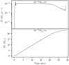 |
Fig. 1 Evolutionary history of the central star. The upper and lower panels show the accretion rate and stellar mass of the representative 10−3 M⊙ yr−1 model, respectively. |
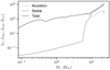 |
Fig. 2 Luminosities of the central star plotted against stellar mass, for the representative 10−3 M⊙ yr−1 model. The stellar, accretion, and total luminosities (as functions of stellar mass) are given by dashed, dotted, and solid lines, respectively. |
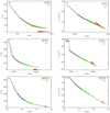 |
Fig. 3 Radius-dependent physical profiles of the three mass-accretion rates used in the chemical models. Panels a to c show temperature profiles as a function of radius, whereas panels d to f show density profiles as a function of radius. Upper panels a and d correspond to the 3.0 × 10⁻³ M⊙ yr−1 mass-accretion rate, middle panels b and e correspond to the 1.0 × 10⁻³ M⊙ yr−1 mass-accretion rate, and the lower panels c and f correspond to the 1.0 × 10⁻⁴ M⊙ yr−1 mass-accretion rate. The black curves represent the final stage-2 simulation time, the green curves represent a stage-2 simulation time corresponding to 100 K for the innermost trajectory of each mass-accretion rate, and the red curves represent the initial stage-2 simulation time. It should be noted that the range for the horizontal axis is different for models of different mass-accretion rates. |
3.2 Chemical results
We focus on the chemical results of ten commonly studied organic molecules: formaldehyde (H2 CO), methanol (CH3OH), ethanol (C2 H5OH), methyl formate (CH3OCHO), glycolaldehyde (CH2OHCHO), dimethyl ether (CH3OCH3), methyl cyanide (CH3CN), ethyl cyanide (C2 H5CN), methyl isocyanide (CH3NC), and vinyl cyanide (C2 H3CN). We discuss fractional abundance and column-density trends in the following subsections.
3.2.1 Fractional abundances
To assess the chemical response to the three different physical models, we generate fractional abundance plots for various COMs with respect to molecular hydrogen, shown in Figs. 5 and 6, with panels ordered in the same way as for the physical conditions in Figs. 3 and 4. Each panel in Fig. 5 corresponds to all trajectories at the final simulation time, whereas each panel in Fig. 6 tracks the innermost trajectory through all simulation times. Generally, COMs become abundant inthe gas-phase at a radius and time corresponding to the temperature at which thermal desorption occurs.
Surface-and ice-mantle abundances are generally static for all molecules until those molecules desorb (Fig. 5). Most COMsform first on grains either in the Stage-1 collapse or early in the Stage-2 warm-up at relatively low temperatures (12–25 K), by hydrogenation or by radical addition. Methanol and formaldehyde, for example, form late in the cold collapse phase by successive hydrogenation of CO. Ethanol forms strongly during the warm-up beginning at about 12 K via addition of CH3 and CH2OH that are produced by photodissociation of methanol and methane, although a substantial amount of ethanol is formed during the cold Stage 1, via methane processing. Reactive radicals such as OH abstract hydrogen atoms from methane to form CH3. Carbon, oxygen, and hydrogen atoms then add to CH3 to form ethanol. Methyl formate and glycolaldehyde begin to form at around 15 K by addition of HCO to CH3O and CH2OH, respectively; the HCO radicals largely derive from solid-phase formaldehyde (H2 CO), while the other two radicals are methanol photoproducts. Methyl cyanide is formed partially early on in the warm-up by addition of CH3 and CN radicals, though most of it forms during the cold Stage 1 via successive hydrogenation of C2 N; methyl isocyanide, on the other hand, is formed by radiative association and subsequent recombination of CH3+ and HCN in the gas phase (Willis et al. 2020) during the warm-up stage. The gas-phase methyl isocyanide accretes on grains, which constitutes the majority of its surface abundance, and then later desorbs at about 100 K. Both ethyl and vinyl cyanide form during the collapse phase via successive hydrogenation of C3 N on the grain/ice surfaces. A more thorough discussion of the formation and destruction mechanisms of these molecules is presented by Barger & Garrod (2020).
For most COMs (except the much more volatile formaldehyde) thermal desorption begins at about 105 K. This corresponds to a final-time radius of 3.0 × 1016 cm (2000 au) for the 3.0 × 10⁻³ M⊙ yr−1 model, 2.8 × 1016 cm (1870 au) for the 1.0 × 10⁻³ M⊙ yr−1 model, and 2.4 × 1016 cm (1600 au) for the 1.0 × 10⁻⁴ M⊙ yr−1 model. Desorption is typically complete by the time a temperature of around 130 K is reached for individual trajectories; peak gas-phase abundances are also achieved at around this temperature for most COMs (see Table 2). Formaldehyde begins to desorb at about 37 K, due to its low binding energy. This corresponds to a radius of 5.9 × 1016 cm (3940 au) for the 3.0 × 10⁻³ M⊙ yr−1 model, 9.4 × 1016 cm (6280 au) for the 1.0 × 10⁻³ M⊙ yr−1 model, and 1.7 × 1017 cm (11 400 au) for the 1.0 × 10⁻⁴ M⊙ yr−1 model.
After desorption occurs, gas-phase abundances are also generally static for all molecules except formaldehyde and methyl isocyanide (Fig. 5); abundances of these molecules decline especially for the 1.0 × 10⁻⁴ M⊙ yr−1 model. Peak gas-phase abundances are generally consistent among the 3.0 × 10⁻³ and 1.0 × 10⁻³ models. However, gas-phase abundances are notably diminished for the 1.0 × 10⁻⁴ M⊙ yr−1 model, especially for formaldehyde, methyl formate, and glycolaldehyde.
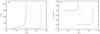 |
Fig. 4 Time-dependent physical profiles of the innermost trajectory in each of the three mass-accretion rates used in the chemical models. Panel a illustrates temperature profiles as a function of time, whereas panel b illustrates density profiles as a function of time. The black curve corresponds to the 3.0 × 10⁻³ M⊙ yr−1 mass-accretion rate, the green curve corresponds to the 1.0 × 10⁻³ M⊙ yr−1 mass-accretion rate, and the red curve corresponds to the 1.0 × 10⁻⁴ M⊙ yr−1 mass-accretion rate. |
Peak gas-phase fractional abundances for the innermost trajectory of each mass-accretion rate model.
3.2.2 Evolution of column densities
In order to assess our results in a format commensurate with observational data, we integrate the absolute abundances of molecules, i.e., n(i), along multiple, parallel lines of sight through the one-dimensional core, at varying offsets from the on-source position, to obtain circularly symmetric column density maps. These maps are then convolved with a gaussian beam (directed on-source) to produce a final value for each molecule. In this study, we compare our results with molecular observations taken toward the high-mass star-forming core Sgr B2(N2). In the review by Jørgensen et al. (2020), observational abundances of various COMs with respect to methanol toward this region were collated from several studies (Belloche et al. 2016, 2017; Müller et al. 2016; Bonfand et al. 2019; Ordu et al. 2019; Willis et al. 2020) based on the EMoCA survey of Belloche et al. (2016). To compare directly with those values, column density maps from the chemical models are convolved using a 1″ beam and an assumed distance to Sgr B2 of 8.34 kpc, following the measurements of Reid et al. (2014). The choice of beam size is intended to approximate the capabilities of ALMA in the 3 mm band.
Plots of the on-source gas-phase column densities of various COMs are given in Fig. 7. Panel a shows column densities obtained at the beginning of Stage 2. Panel b gives Stage-2 column densities calculated at a time corresponding to a temperature of 100 K for the innermost trajectory of each model. This occurs at 7.17 × 10³, 2.47 × 10⁴, and 2.88 × 10⁵ yr, respectively, for the 3.0 × 10⁻³, 1.0 × 10⁻³, and 1.0 × 10⁻⁴ M⊙ yr−1 models (see Fig. 3). Panel c shows column densities at the final Stage-2 simulation time for each mass-accretion rate model.
The column densities at the initial Stage-2 simulation time (Fig. 7) are all low compared with typical observational values, as would be expected, and typically range from 105 to 1010 cm−2. This owes to the fact that the gas and grain temperatures are between 8 and 14 K at this time. Consequently, complex molecules do not have sufficient energy to thermally desorb from the grains, and the gas-phase column densities are low. However, when a temperature of 100 K is reached by the innermost trajectory, most COMsare beginning to desorb from the grains, and the column densities in panel b rise to values typically ranging from 1012 to 1015 cm−2. At the final simulation time, all COMs have desorbed into the gas phase in a large fraction of the simulated trajectories, and column densities typically reach their highest values, which are in the approximate range 1016 to 1019 cm−2.
Locally, complex molecules tend to become more abundant in the gas phase as the simulation proceeds, which leads to higher overall column densities. By the final simulation time, the column densities of the 3.0 × 10⁻³ and 1.0 × 10⁻³ M⊙ yr−1 models are generally within an order of magnitude of each other (Fig. 7). However, column densities in the 1.0 × 10⁻⁴ M⊙ yr−1 model are consistently much lower by several orders of magnitude, partially because of the lower gas column density associated with the lower mass-accretion rate. However, the major cause of this shortfall for some species is the far lower ice abundance built up during Stage 1, which limits the quantities of COMs that can be formed on the grains. The methanol ice abundance is lower by around an order of magnitude in the low mass-accretion rate model (see Fig. 6), while the abundances of carbon monoxide and formaldehyde ice are negligible in that model.
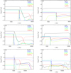 |
Fig. 5 Spatially dependent fractional abundance plots (with respect to H2) for select COMs, at the end of each accretion-rate model. Panels a to c show fractional abundances for methanol (black), ethanol (blue), methyl formate (green), glycolaldehyde (yellow), and dimethyl ether (red). Panels d to f show fractional abundances for formaldehyde (black), methyl cyanide (blue), ethyl cyanide (green), methyl isocyanide (yellow), and vinyl cyanide (red). Upper panels a and d correspond to the 3.0 × 10⁻³ M⊙ yr−1 mass-accretion rate, middle panels b and e correspond to the 1.0 × 10⁻³ M⊙ yr−1 mass-accretion rate, and lower panels c and f correspond to the 1.0 × 10⁻⁴ M⊙ yr−1 mass-accretion rate. Solid lines correspond to gas-phase abundances, whereas dashed lines correspond to surface/ice-mantle abundances. It should be noted that the range for the horizontal axis is different for models of different mass-accretion rates. |
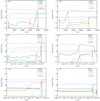 |
Fig. 6 Time-dependent fractional abundance plots (with respect to H2) for select COMs, for the innermost trajectory in each accretion-rate model. Panels a through c show all-time innermost trajectory fractional abundances for methanol (black), ethanol (blue), methyl formate (green), glycolaldehyde (yellow), and dimethyl ether (red). Panels d through f show all-time innermost trajectory fractional abundances for formaldehyde (black), methyl cyanide (blue), ethyl cyanide (green), methyl isocyanide (yellow), and vinyl cyanide (red). Upper panels a and d correspond to the 3.0 × 10⁻³ M⊙ yr−1 mass-accretion rate, middle panels b and e correspond to the 1.0 × 10⁻³ M⊙ yr−1 mass-accretion rate, and lower panels c and f correspond to the 1.0 × 10⁻⁴ M⊙ yr−1 mass-accretion rate. Solid lines correspond to gas-phase abundances, whereas dashed lines correspond to surface/ice-mantle abundances. It should be noted that the range for the horizontal axis is different for models of different mass-accretion rates. |
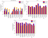 |
Fig. 7 On-source column densities for select COMs using a 1 arcsec beam convolution. The red bars illustrate column densities for the 3.0 × 10⁻³ M⊙ yr−1 model, the blue bars illustrate column densities for the 1.0 × 10⁻³ M⊙ yr−1 model, and the orange bars illustrate column densities for the 1.0 × 10⁻⁴ M⊙ yr−1 model. Panel a shows column densities for the initial stage-2 simulation time, panel b shows column densities for stage-2 simulation times that correspond to a temperature of 100 K, and panel c shows column densities for the final stage-2 simulation time. It should be noted that the ranges for the vertical axis differ for all panels. |
3.2.3 Column densities for constant source mass
While it is instructive to consider the fractional abundances and column densities at various times throughout our models, each mass-accretion rate necessarily leads to a somewhat different physical outcome. In order to allow a more direct comparison between each physical model, we also consider the column densities produced by each at certain fixed masses achieved by the central source. To avoid differing beam-dilution effects between different accretion-rate models, based on their varied spatial extents, these on-source column densities are presented without convolution; they therefore represent column densities along a pencil beam.
Unconvolved on-source column densities for source masses 5, 10, 15, 20, and 23 M⊙ are shown in Fig. 8 for various COMs; the last value is the highest achieved in the 1.0 × 10⁻³ M⊙ yr−1 model. For all three mass-accretion rates, the column densities of all molecules within a given model generally increase with increasing source mass. This owes to the fact that higher masses correspond to later simulation times; consequently, the overall gas column densities are higher due to the isotropic collapse, while the greater accretion and stellar luminosities (see Fig. 2 for example) also lead to higher temperatures that are conducive to COM production and desorption.
The 3.0 × 10⁻³ M⊙ yr−1 model generally features the highest column densities for all source masses, with the exception of 23 M⊙ (Fig. 8). The 1.0 × 10⁻⁴ model consistently features the lowest column densities. For instance, at 23 M⊙ mass, column densities are as many as 7 orders of magnitude lower compared to the other two models. This trend is caused by three effects. First, a higher mass-accretion rate leads to a higher gas column density. Second, and perhaps more importantly, a higher mass-accretion rate leads to a higher accretion luminosity for a given stellar mass, which, in turn, leads to higher temperatures for a given spatial extent between models, especially at relatively early times when the accretion luminosity dominates the stellar luminosity (see Fig. 2 for an illustration). Both effects lead to higher COM column densities for higher accretion rate models. Finally, as described in the previous subsection, the weaker ice production for certain species in the lowest accretion-rate model, caused by the low gas densities of all trajectories throughout most of the model run, results in lower COM production. This is particularly the case for COMs bearing HCO functional groups, which would be expected to form preferentially during the intermediate temperature regime (i.e., 20–100 K), fed by the photodissociation of H2 CO in the ice – or, failing that, the hydrogenation of CO. The low mass-accretion rate model in fact spends longer than the other models in this temperature regime, due to the slower evolution of the source, but this effect is insufficient to compensate for the much lower abundances of important solid-phase molecules.
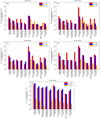 |
Fig. 8 Unconvolved on-source column densities for select COMs. The red bars illustrate column densities for the 3.0 × 10⁻³ M⊙ yr−1 model, the blue bars illustrate column densities for the 1.0 × 10⁻³ M⊙ yr−1 model, and the orange bars illustrate column densities for the 1.0 × 10⁻⁴ M⊙ yr−1 model. Panel a corresponds to stage-2 simulation times for which each model has a mass of 5 M⊙, panel b corresponds to times for which each model has a mass of 10 M⊙, panel c corresponds to times for which each model has a mass of 15 M⊙, panel d corresponds to times for which each model has a mass of 20 M⊙, and panel e corresponds to times for which each model has a mass of 23 M⊙. |
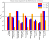 |
Fig. 9 Comparison among observed column densities for select COMs toward Sgr B2(N2) and those modeled on-source using a 1 arcsec beam convolution. The red bars illustrate column densities for the 3.0 × 10⁻³ M⊙ yr−1 model, the blue bars illustrate column densities for the 1.0 × 10⁻³ M⊙ yr−1 model, and the orange bars illustrate column densities for the 1.0 × 10⁻⁴ M⊙ yr−1 model. Rmod represents modeled column density ratios relative to methanol, and Robs represents observed column density ratios relative to methanol (Jørgensen et al. 2020). The horizontal line indicates a value of 1 on the y-axis. |
3.2.4 Comparing observed and modeled column densities
A comparison of our modeled column densities with those observed toward Sgr B2(N2) (Jørgensen et al. 2020, and references therein) is presented in Fig. 9. For each species, a quantity Rmod is calculated, which is equal to the ratio of the convolved column density of that species to that of methanol, as determined from the models. A similar quantity, Robs, represents the observed column densities as a fraction of the observed methanol abundance. Figure 9 shows the ratio Rmod/Robs for each species. The comparison with respect to methanol allows the further removal of possible confounding physical effects due to differences between the three accretion-rate models and/or Sgr B2(N2) itself; methanol should track well with the overall column density of the dense, hot gas within the core. The horizontal blue line in the plot represents a value of 1, i.e., Rmod = Robs. The uncertainties on the observational values with which we compare are dependent on multiple considerations involved in producing a simulated spectrum for each molecule; these include the rotational temperature and assumed size of the emitting region, blending with other molecular lines and U-lines, the assumption of LTE for the populations of vibrationally excited states (affecting the partition function), and systematic errors associated with the existence of spatial gradients in the gas density, temperature, and molecular abundances. Overall uncertainties in the observed molecular column densities could be as high as 30–50% in some cases (Belloche, priv. comm.). Bonfand et al. (2019) suggest, in their Appendix A, a blanket uncertainty of 30% for values toward Sgr B2(N2). This would provide an uncertainty in the quotient Robs of ~ 42%.
The comparison for ethanol is the best of any COM surveyed as the agreement among Robs and Rmod is within a factor of ten for all mass-accretion-rate models (Fig. 9), with an even closer match for the two highest mass-accretion rates. The comparison for methyl formate and formaldehyde is also good for the 3.0 × 10⁻³ and 1.0 × 10⁻³ M⊙ yr−1 models as the agreement is also within a factor of ten. However, our modeled column densities for these COMs are severely under-produced for the 1.0 × 10⁻⁴ M⊙ yr−1 model as Rmod is more than two magnitudes lower than Robs. All other COMs surveyed generally disagree with Robs values by a factor of 10−100 for all models. Furthermore, Rmod values are consistently lower than corresponding Robs values, with the exception of a few cases.
4 Discussion
4.1 Fractional abundances
A notable departure from previous work shown by these models is the exceptionally weak dependence of the chemistry on gas-phase processes. Gas-phase abundances are largely static after species desorb, for all models/timescales. Earlier studies (e.g., Garrod 2013; Barger & Garrod 2020), show gas-phase abundances that tend to diminish noticeably, especially over long timescales, due to destruction by ionic species. The difference may be partially attributed to the present models’ incorporation of proton-transfer reactions with NH4+, following the suggestion of Taquet et al. (2016), which allows protonated COMs to be de-protonated without destroying their structure, as would typically be the case if electronic recombination were the only destruction mechanism for those species. The addition of this pathway diminishes a major gas-phase destruction route for COMs. Another reason for the relatively constant COM abundances is that, once a parcel of gas reaches a temperature high enough for COMs to be thermally desorbed from the grains, it is already close to the central stellar object and falls into the star quickly, allowing little time for gas-phase reactions. As may be seen from Table 1, the time period available for gas-phase chemistry above 100 K is on the order of just a few thousand years. The corresponding timescales of the past models ranged from a few 104 years to more than half a million years.
An exception to this behavior is formaldehyde (H2 CO), which is destroyed in the gas phase (Figs. 5 and 6, panels d-f) due to reactions with atomic hydrogen and oxygen. This effect is especially pronounced in the 1.0 × 10⁻⁴ M⊙ yr−1 model (panel f), owing to much higher abundances of both atomic hydrogen and oxygen. The low mass-accretion rate of this model is achieved by assuming low gas densities at the beginning of the Stage-2 collapse; this means that gas-phase reactions and freeze-out onto dust grains are less effective, while the visual extinction is also very low for trajectories starting at greater radii. Accordingly, atomic species are much more abundant in the gas phase for this model. Formaldehyde also desorbs from the grains at a lower temperature than most COMs, providing a longer period for gas-phase chemistry. As noted in previous work, the release of formaldehyde before the majority of other species also makes formaldehyde the main reaction partner for destructive ions, expediting its destruction even in the higher mass-accretion-rate models.
Like formaldehyde, methyl isocyanide (CH3NC) is destroyed in the gas phase due to reaction with atomic hydrogen (Figs. 5 and 6, panels d-f), in line with the behavior assumed for gas-phase destruction of HNC (Graninger et al. 2014; Willis et al. 2020). This effect is especially pronounced in the 1.0 × 10⁻⁴ M⊙ yr−1 model, due to its large abundance of atomic hydrogen.
The absolute and relative abundances of the structural isomers methyl formate (CH3OCHO) and glycolaldehyde (CH2OHCHO) are of particular observational interest in the hot core regime. Gas- and solid-phase methyl formate and glycolaldehyde abundances are severely diminished (by 3 to 4 orders of magnitude) in the 1.0 × 10⁻⁴ M⊙ yr−1 model (Figs. 5 and 6, panel c) compared to the other two mass-accretion-rate models. This is primarily caused by a scarcity of HCO on the dust grains, which otherwise leads to the formation of these species via radical addition with CH3O/CH2OH. At early times in the models, at very low temperatures, CO from the gas phase is accreted onto the grains, where it is converted to formaldehyde (H2 CO) and thence to methanol (CH3OH) via reactions with atomic H that originates in the gas phase. In the lowest mass-accretion rate model, the slow build-up of the ices (caused by low gas densities) combined with the high abundance of gas-phase H leads to the more complete hydrogenation of CO on the grain surfaces. This removes formaldehyde from the ice mantles, which could otherwise be photodissociated (or chemically processed) later on to produce the HCO needed for the above COMs to be formed. The high degree of hydrogenation to form methanol also strongly manifests in the abundance of CO left in the ice; fractional abundances with respect to total hydrogen of around 10−7 to 10−9 are achievedat the end of Stage-1 evolution for the lowest accretion-rate model, while values on the order of 10−5 are reached in the two higher accretion-rate models. The low value in the low accretion-rate models is contrary to typical observational values (e.g., Boogert et al. 2015), while the other two models are in good agreement with observations. Table 3 shows modeled surface column density ratios relative to water for common surface species. We find that for the two highest mass-accretion-rate models, column density ratios are on the order of 10−1 to 10−2, which agree well with the ratios of Boogert et al. (2015), which are typically on the same order for CO, CO2, CH4, NH3, and CH3OH. However, our ratios for the 1.0 × 10⁻⁴ M⊙ yr−1 model are on the order of 10−4 or less, which is severely diminished compared to observations.
In general, the peak gas-phase abundances tend to be similar between the 3.0 × 10⁻³ and 1.0 × 10⁻³ M⊙ yr−1 models for the innermost trajectory (see Table 2). This similarity in the two higher-rate models is related to their more similar mass-accretion rates and the associated physical and time-related conditions under which chemistry occurs. While the overall timescale of the low accretion-rate model is longer than the others, it is still approximately in inverse proportion to the lower final central density of that model (Table 1). However, the densities at early times in each model vary much more strongly than this; as seen in Fig. 4, the innermost trajectory in the low mass-accretion-rate model spends most of its time at gas densities on the order of 104 cm−3, while the other models have densities for their innermost trajectories that are a factor 100 or 1000 higher. Thisfar outweighs the longer timescale available to the low mass-accretion-rate model. As a result, the amount of chemical evolution and overall ice build-up is substantially lower in the 1.0 × 10⁻⁴ M⊙ yr−1 case. Also, while this model spends a much longer period of time at temperatures below 100 K than the other two (approximately 288 000 yr vs. 24 000 and 7000 yr), it spends a shorter time above (approximately 1600 yr vs. 4300 and 2900 yr), limiting the time available forany post-desorption, gas-phase production of COMs (in those cases where such processes exist, such as for dimethyl ether, which has a viable formation route involving the reaction of methanol with protonated methanol).
The only area in which the chemical evolution of the low mass-accretion-rate model is favored is in the cosmic ray-induced photo-processing of the ice mantles, which produces reactive radicals. In spite of the lower abundance of solid-phase molecules as described above, the long timescale for this model allows the ices to experience a larger overall fluence of CR-induced UV photons, and therefore a larger degree of processing of the solid-phase material that is present. Dimethyl ether appears to be the main beneficiary of this effect; it can be formed solely from methanol dissociation products (CH3 and CH3O), so the lack of H2CO in the ices in the low mass-accretion-rate model is less important, while the longer timescale more than counterbalances the lower methanol abundance in the ice. In contrast to past models, CH3OCH3 is not formed in the gas phase in any substantial amount in any of the models, due to the short timescales available to gas-phase COM chemistry at temperatures greater than 100 K.
Observed ethanol abundances with respect to methanol are also well reproduced in all models; however, this molecule is formed efficiently at low temperatures in each, reducing the importance of its later enhancement at intermediate temperatures during Stage 2. In the low mass-accretion-rate model, the production of ethanol via methanol photolysis is more substantial and, as with its structural isomer dimethyl ether, it benefits from the large abundance of methanol combined with the long timescale for photodissociation.
The abundances of CH3CN and C2 H5CN are little different between the various models, and are even marginally enhanced in the lowest accretion-rate case. Their production through mechanisms that involve grain-surface hydrogenation of gas-phase produced species (such as HCCN and HC3N) makes the abnormally large abundance of gas-phase H in the low mass-accretion rate model an advantage, rather than a hindrance as in the case of HCO-group-bearing molecules.
Select modeled grain-surface column density ratios of solid-phase molecules relative to water for all three mass-accretion rates, calculated at the end of stage 1, using an on-source position with no beam convolution.
On-source column densities (cm−2) of C2 H4O2 isomers for final Stage 2 simulation times using innermost trajectories.
4.2 Column densities
The calculation of column densities provides a more complete picture of the behavior of the chemistry in the simulated hot cores, and allows direct comparison with observations in a way that past models using simple physical evolution treatments have been unable to do. However, some similar trends persist from past models; notably, the amount of glycolaldehyde produced continues to exceed that of methyl formate, contrary to observations. The EMoCA survey data demonstrate a roughly 10:1 ratio of CH3OCHO:CH2OHCHO for Sgr B2(N2), and the PILS data for the solar-type YSO IRAS 16293B indicate a similar ratio, while the models produce column densities with this ratio inverted. However, the column density ratio of methyl formate to methanol agrees well with observational values in the two highest mass-accretion-rate models. Excessive glycolaldehyde production is therefore the likely culprit. Its overproduction by a factor around 100 still remains to be reconciled with observations.
An outstanding problem in astrochemical modeling pertains to constraining the modeled abundances of the C2 H4O2 isomers: methyl formate, glycolaldehyde, and acetic acid (CH3COOH) (Laas et al. 2011). Table 4 illustrates on-source column densities for these species at the end of the Stage 2 simulation for the innermost trajectories of the three mass-accretion-rate models. El-Abd et al. (2019) report a strong correlation among column density ratios of methyl formate relative to acetic acid with respect to source mass: Higher-mass objects tend to yield higher ratios. However, our column density ratios indicate a strong correlation among these ratios with respect to the mass-accretion rate: As the mass-accretion rate increases, the methyl formate-to-acetic acid ratio increases (2.7 × 10⁻⁶, 3.8 × 10⁻¹, and 1.3 × 100 for 3.0 × 10⁻³ M⊙ yr−1, 1.0 × 10⁻³ M⊙ yr−1, and 1.0 × 10⁻⁴ M⊙ yr−1, respectively). Though our ratios increase with the mass-accretion rate, they do not correlate well with the final source mass (see Table 1, Col. 4).
El-Abd et al. (2019) found that in general, large ratios of methyl formate relative to glycolaldehyde tend to correspond exclusively to high-mass star-forming regions, whereas lower ratios correspond to mixed source masses. The authors suggest that a parameter other than source mass may be responsible for the trend in these ratios. From Table 4, the ratios of methyl formate relative to glycolaldehyde are 3.3 × 10⁻¹ for the 1.0 × 10⁻⁴ M⊙ yr−1 model, 4.3 × 10⁻¹ for the 1.0 × 10⁻³ M⊙ yr−1 model, and 4.8 × 10⁻¹ for the 3.0 × 10⁻³. This illustrates a moderate positive correlation among these ratios with the mass-accretion rate. It may be that the overall column density ratios are more strongly influenced by the overall accretion rate instead of source mass.
According to Fig. 8, at constant source mass there does not appear to be consistency among column densities for all three mass-accretion-rate models. Each of the five source masses illustrates a variety of column density values among the models for any particular species. This is due to the fact that although the source mass is constant, each model reflects a different simulation time, and thus temperature. Gas-phase fractional abundances, and thus column densities, are particularly temperature-dependent through the thermal ejection of the ice mantles, and the temperatures of these models are inconsistent at any given source mass. This is especially pronounced at the 23 M⊙ comparison point. The COM column densities of the 1.0 × 10⁻⁴ M⊙ yr−1 model are significantly lower than the other two models because the spatial extents of the temperature regimes needed for COMs to desorb are smaller, while the column density of the gas is also lower because of the lower local gas densities. These absolute column density values provide further indication that the low accretion-rate models do not provide appropriate physical conditions to match observable features of high-mass sources. However, between the two highest mass-accretion-rate models, the 23 M⊙ molecular column densities are in fairly close agreement, with divergences generally favoring slightly higher values for the intermediate-rate model. The similarities between the models under these comparable conditions therefore make it unlikely that relative chemical abundances alone could be used as an indicator of the mass-accretion rate with any degree of precision for evolved hot-core sources.
However, one notable feature is apparent in the 20 M⊙ column densities; while most values are comparable between the two highest mass-accretion-rate models, the abundances of methyl formate and dimethyl ether are larger in the highest-rate model by many orders of magnitude. This effect is related to the slightly earlier release of these two species compared to most other COMs, combined with the larger extent of each temperature regime in the high accretion-rate model; this effect just happens to be captured at the correct moment in the 20 M⊙ comparison. The column densities at this moment are nevertheless more than two orders of magnitude lower than their peak values seen at 23 M⊙, so any possibleobservable effect in hot cores might not be easily observable, due to the overall weaker molecular emission at this stage.
Our modeled column density ratios of CH3NC to CH3CN toward Sgr B2(N2) are 0.15, 0.17, and 1.2, respectively, for the 3.0 × 10⁻³, 1.0 × 10⁻³, 1.0 × 10⁻⁴ M⊙ yr−1 models. These values are relatively high compared to the best fit results toward Sgr B2(N) presented by Willis et al. (2020), which are 1.3 × 10⁻² and 1.4 × 10⁻³. Our values are also higher than the observational ratio of 4.5 × 10⁻³ toward Sgr B2(N2) reported in the table presented by Jørgensen et al. (2020). This could indicate that the post-desorption timescales available for gas-phase chemistry to destroy CH3NC are too short in the present models.
4.3 Shortcomings of the physical model
Many of themodeled column densities considered in the present work are consistently lower than those observed toward Sgr B2(N2) (Fig. 9). Although many uncertainties remain in our chemical network (see below), the fact that the column densities are lower for so many species suggests that a systematic inaccuracy may exist in the underlying physical structure produced by the one-dimensional dynamical simulations, at least for the purposes of comparison with the Galactic Center source Sgr B2(N2). In all mass-accretion rate cases, the final gas densities of our models are lower than those determined for Sgr B2(N2) (Bonfand et al. 2019) by a couple of orders of magnitude, which could account for the comparatively lower gas column densities. Accordingly, comparing our results with those for Sgr B2(N2) may not be entirely appropriate (although comparisons with column densities normalized to methanollikely improve any purely spatial discrepancies). It is also possible that the cosmic-ray ionization rate in that region is substantially higher than the standard interstellar value that we assume here (e.g., van der Tak et al. 2006). Alternatively, the failure may indicate that Sgr B2 (N2) accretes at a much higher rate than 1.0 × 10⁻⁴ M⊙ yr−1.
A clear chemical failure caused by the physical setup used in the lowest mass-accretion-rate model is the weak ice production caused by the lingering low gas densities, as well as the extreme degree of hydrogenation of CO on the grains. In this particular model, the hot-core stage follows on rapidly from a long, low-density phase with no substantial period of ice production in between. A more sophisticated treatment may be required for the early stages of evolution of the 1.0 × 10⁻⁴ M⊙ yr−1 case.
There is also very little time for hot gas-phase chemistry to occur, after the desorption of dust-grain ice mantles, before infall of the trajectory onto the central source takes place, ending the chemical evolution. The CH3NC/CH3CN ratio could indeed indicate that more time for gas-phase COM destruction is required, even for the low-rate model, although the destruction rate of the isocyanide through H-atom reactions is poorly constrained due to an uncertain activation energy barrier. A solution to this physical problem may supercede any simple adjustments to the basic model; instead a more complete transition to a greater than one-dimensional dynamical treatment may be required,in which, for example, additional support from rotation and/or magnetic fields could be properly modeled.
The formation of a disk in the presence of rotation is expected to significantly change the gas dynamics and temperature distribution.For example, the disk would allow the radiation from the central star to escape more easily in the lower density regions nearthe poles, which introduces an anisotropy in the radiative heating of the circumstellar material. It is needed to explain the recent observations of Csengeri et al. (2019), which have identified specific structures in the inner envelope of a high-mass protostar traced by COMs. They find chemical differentiation between O- and N-bearing species (specifically nitriles), associated with distinct regions corresponding to accretion shocks onto a disk on the one hand, and the more general inner envelope region on the other. They suggest that the temperature differences between these regions may be responsible for the chemical differences. Our present model is unable to treat these observed physical features.
4.4 Shortcomings of the chemical models
As noted above, while some chemical abundances are broadly in line with observational values, there remain inconsistent behaviors – such as the ratios between methyl formate and its structural isomers – that are largely unaltered by the use of a new physical model. We note that, over the past several years, an increasing focus has fallen upon the proposed formation of COMs, as well as simpler species such as CO2 (Garrod & Pauly 2011), on dust-grain surfaces through so-called nondiffusive mechanisms (see Jørgensen et al. 2020). Laboratory evidence by Fedoseev et al. (2015), as well as their follow-up studies, has shown that oxygen-bearing COMs may be formed on cold ice surfaces in tandem with the production of formaldehyde and/or methanol through the hydrogenation of CO. The occasional production of radical intermediates in close proximity on the surface leads to reaction, without the requirement for the thermal diffusion of large radicals; the rapid diffusion of H atoms alone, even at very low temperatures, is thought to be sufficient to initiate this process.
Jin & Garrod (2020) recently proposed a generic framework for the inclusion in chemical models of various nondiffusive grain-surface reaction processes, including not only the reaction mechanism described above (which they label the three-body mechanism), but also photon-initiated reactions within the ice mantle that do not require diffusion of reactants within the bulk ice. These treatments appear promising as an explanation for the existence of COMs in the gas-phase of cold, pre-stellar cores (Bacmann et al. 2012; Jiménez-Serra et al. 2016), as the result of nonthermal desorption of grain surface-produced molecules. As suggested by Bacmann et al. (2012) the detection of such species in the very early stages of star formation (albeit, in that case, toward low-mass cores) indicates that at least some of the hot, complex organic material observed later on has a cold origin. It is plausible indeed that the abundances studied in the present work would be affected by the inclusion of nonthermal surface and bulk-ice mechanisms into the chemical model. The treatments of Jin & Garrod (2020), which have been explored thus far only under cold conditions, were developed in tandem with the present models. They are, however, currently being applied explicitly to hot-core physical conditions (Garrod et al. 2021), and will likely be included in the next round of our own combined chemical/physical simulations of hot cores.
The uncertainty in the binding energies of certain observable species, and in the binding energies and diffusion barriers of radical species from which they may form, are also a possible source of error (e.g., Penteado et al. 2017). The relativerates of diffusion of surface radicals are especially difficult to determine directly from experiment, so calculations of the barriers against diffusion may be the most effective means to obtain such information for chemical kinetic models (Wakelam et al. 2017).
5 Conclusions
The hot-core chemical modeling results presented here are the first to adopt an underlying physical treatment derived from a self-consistent RHD simulation of the density and temperature progression over time. They represent the first iteration of our ongoing effort to couple more closely the physics and chemistry in these molecule-rich sources. The main conclusions of this study are enumerated below:
Gas-phase fractional abundances of the COMs we surveyed tend to remain static after thermal desorption occurs. This effect contrasts to the gradual diminishing of abundances over time from previous modeling studies, and may be attributed to the short time-interval between COM desorption and infall onto the star, and, to a lesser extent, to the incorporation into our chemical network of proton-transfer reactions between protonated COMs and ammonia;
Fractional abundances in the 3.0 × 10⁻³ and 1.0 × 10⁻³ M⊙ yr−1 models are similar, due to the fact that the physical behavior of these models is qualitatively similar. The much lower fractional abundances achieved in the 1.0 × 10⁻⁴ M⊙ yr−1 model are mainly due to the requirement to have low gas densities throughout the core during the initial cold stage, in order to achieve the specified mass-accretion rate; the much lower densities in these models lead to diminished ice abundances prior to the hot stage, as well as ice chemical compositions that do not agree well with typical observed values. More general disagreements in total gas column densities are attributable to the lower local densities and the smaller radius of temperatures capable of initiating thermal desorption of COMs, which are caused by the lower accretion luminosity of this model;
Comparison of the evolution of the models as a function of source mass shows COM column densities increasing as the source grows, due to molecules thermally desorbing from grains as temperatures grow, induced by rising stellar and accretion luminosities;
Within the limited set of physical models tested here, for a constant source mass the two highest mass-accretion-rate models show only modest differences. The lowest-rate model shows different behavior, due to its qualitatively different physical evolutionary behavior;
Comparison of convolved column densities for selected species with observed values indicates systematic underproduction, likely caused simply by a divergence between the adopted physical conditions in the models and those of Sgr B2(N2);
While providing a nominally better physical model, the use of a self-consistent one-dimensional dynamical treatment leads to extremely short post-desorption timescales that allow little room for hot gas-phase chemistry;
We believe that the use of a two-dimensional radiation-hydrodynamics treatment will provide a physical picture that is more in line with the expected observational structures within high-mass star-forming cores.
Recent developments in grain-surface and bulk-ice chemical kinetic treatments (Jin & Garrod 2020; Garrod et al. 2021) may provide further improvements in the model results that cannot be achieved by adjustments to the physical model alone. The production of some COMs at very low temperatures, as indicated by those treatments, demands that the dynamics of the very earliest stages of hot-core evolution be given as much attention as the later, hotter stages.
Acknowledgements
We thank the referee, T. Grassi, for a very constructive review that greatly improved this manuscript. We thank A. Belloche for helpful discussions. This work is funded by a grant from the NASA Astrophysics Theory Program (grant number 80NSSC18K0558). Simulations were conducted using the University of Virginia’s Rivanna supercomputer cluster.
Appendix A Supplementary table
Newly added gas-phase reactions involving proton transfer from protonated COMs to ammonia are listed along with their rate parameters in Table A.1.
Relevant recombination reactions with protonated ammonia and rate-coefficient parameters, following Taquet et al. (2014).
References
- Bacmann, A., Taquet, V., Faure, A., et al. 2012, A&A, 541, L12 [NASA ADS] [CrossRef] [EDP Sciences] [Google Scholar]
- Barger, C. J., & Garrod, R. T. 2020, ApJ, 888, 38 [NASA ADS] [CrossRef] [Google Scholar]
- Belloche, A., Müller, H. S. P., Garrod, R. T., et al. 2016, A&A, 587, A91 [NASA ADS] [CrossRef] [EDP Sciences] [Google Scholar]
- Belloche, A., Meshcheryakov, A. A., Garrod, R. T., et al. 2017, A&A, 601, A49 [NASA ADS] [CrossRef] [EDP Sciences] [Google Scholar]
- Belloche, A., Garrod, R. T., Müller, H. S. P., et al. 2019, A&A, 628, A10 [NASA ADS] [CrossRef] [EDP Sciences] [Google Scholar]
- Bohlin, R. C., Savage, B. D., & Drake, J. F. 1978, ApJ, 224, 132 [NASA ADS] [CrossRef] [Google Scholar]
- Bonfand, M., Belloche, A., Garrod, R. T., et al. 2019, A&A, 628, A27 [NASA ADS] [CrossRef] [EDP Sciences] [Google Scholar]
- Boogert, A. C. A., Gerakines, P. A., & Whittet, D. C. B. 2015, ARA&A, 53, 541 [Google Scholar]
- Brogan, C. L., Hunter, T. R., Cyganowski, C. J., et al. 2016, ApJ, 832, 187 [NASA ADS] [CrossRef] [Google Scholar]
- Chang, P., Davis, S. W., & Jiang, Y.-F. 2020, MNRAS, 493, 5397 [Google Scholar]
- Charnley, S. B., Kress, M. E., Tielens, A. G. G. M., & Millar, T. J. 1995, ApJ, 448, 232 [NASA ADS] [CrossRef] [Google Scholar]
- Csengeri, T., Belloche, A., Bontemps, S., et al. 2019, A&A, 632, A57 [NASA ADS] [CrossRef] [EDP Sciences] [Google Scholar]
- Cuppen, H. M., Walsh, C., Lamberts, T., et al. 2017, Space Sci. Rev., 212, 1 [Google Scholar]
- Davis, S. W., & Gammie, C. F. 2020, ApJ, 888, 94 [Google Scholar]
- El-Abd, S. J., Brogan, C. L., Hunter, T. R., et al. 2019, ApJ, 883, 129 [CrossRef] [Google Scholar]
- Fedoseev, G., Cuppen, H. M., Ioppolo, S., et al. 2015, MNRAS, 448, 1288 [NASA ADS] [CrossRef] [Google Scholar]
- Garrod, R. T. 2008, A&A, 491, 239 [NASA ADS] [CrossRef] [EDP Sciences] [Google Scholar]
- Garrod, R. T. 2013, ApJ, 765, 60 [Google Scholar]
- Garrod, R. T., & Pauly, T. 2011, ApJ, 735, 15 [NASA ADS] [CrossRef] [Google Scholar]
- Garrod, R. T., & Widicus Weaver, S. L. 2013, Chem. Rev., 113, 8939 [Google Scholar]
- Garrod, R. T., & Herbst, E. 2006, A&A, 457, 927 [NASA ADS] [CrossRef] [EDP Sciences] [Google Scholar]
- Garrod, R. T., Wakelam, V., & Herbst, E. 2007, A&A, 467, 1103 [NASA ADS] [CrossRef] [EDP Sciences] [Google Scholar]
- Garrod, R. T., Belloche, A., Müller, H. S. P., & Menten, K. M. 2017, ApJ, 601, A48 [Google Scholar]
- Garrod, R. T., Jin, M., Matis, K. M., et al. 2021, ApJS, submitted [Google Scholar]
- Graninger, D. M., Herbst, E, Öberg, K. I., & Vasyunin, A. I. 2014, ApJ, 787, 74 [NASA ADS] [CrossRef] [Google Scholar]
- Hasegawa, T. I., & Herbst, E. 1993, MNRAS, 263, 589 [NASA ADS] [CrossRef] [Google Scholar]
- Herbst, E., & Leung, C. M. 1986, ApJ, 310, 378 [NASA ADS] [CrossRef] [Google Scholar]
- Herbst, E., & van Dishoeck, E. F. 2009, ARA&A, 47, 427 [NASA ADS] [CrossRef] [Google Scholar]
- Hosokawa, T., & Omukai, K. 2009, ApJ, 691, 823 [NASA ADS] [CrossRef] [Google Scholar]
- Jiang, Y.-F., Stone, J. M., & Davis, S. W. 2019, ApJ, 880, 67 [NASA ADS] [CrossRef] [Google Scholar]
- Jiménez-Serra, I., Vasyunin, A. I., Caselli, P., et al. 2016, ApJ, 830, L6 [Google Scholar]
- Jin, M., & Garrod, R. T. 2020, ApJS, 249, 26 [Google Scholar]
- Jørgensen, J. K., Belloche, A., & Garrod, R. T. 2020, ARA&A, 58, 1 [Google Scholar]
- Kuiper, R., Klahr, H., Beuther, H., et al. 2010, ApJ, 722, 1556 [CrossRef] [Google Scholar]
- Laas, J. C., Garrod, R. T., Herbst, E., & Widicus Weaver, S. L. 2011, ApJ, 728, 71 [NASA ADS] [CrossRef] [Google Scholar]
- Li, Z.-Y., Krasnopolsky, R., & Shang, H. 2011, ApJ, 738, 180 [NASA ADS] [CrossRef] [Google Scholar]
- Mihalas, D., & Mihalas, B. W. 1984, Foundations of radiation hydrodynamics New York, Oxford University Press, 1984, 731 p [Google Scholar]
- Millar, T. J., Herbst, E., & Charnley, S. B. 1991, ApJ, 369, 147 [NASA ADS] [CrossRef] [Google Scholar]
- Müller, H. S. P., Belloche, A., Xu, L.-H., et al. 2016, A&A, 587, A92 [NASA ADS] [CrossRef] [EDP Sciences] [Google Scholar]
- Nakano, T., Nishi, R., & Umebayashi, T. 2002, ApJ, 573, 199 [NASA ADS] [CrossRef] [Google Scholar]
- Nejad, L. A. M., Williams, D. A., & Charnley, S. B. 1990, ApJ, 246, 183 [Google Scholar]
- Öberg, K. I., Garrod, R. T., van Dishoeck, E. F., & Linnartz, H. 2009, A&A, 504, 891 [NASA ADS] [CrossRef] [EDP Sciences] [Google Scholar]
- Ordu, M. H., Zingsheim, O., Belloche, A., et al. 2019, A&A, 630, C1 [EDP Sciences] [Google Scholar]
- Penteado, E. M., Walsh, C., & Cuppen, H. M. 2017, ApJ, 844, 71 [NASA ADS] [CrossRef] [Google Scholar]
- Reid, M. J., Menten, K. M., Brunthaler, A., et al. 2014, ApJ, 783, 130 [Google Scholar]
- Shu, F. H. 1977, ApJ, 214, 488 [Google Scholar]
- Stone, J. M., Tomida, K., White, C. J., et al. 2020, ApJS, 249, 4 [Google Scholar]
- Taquet, V., Charnley, S. B., & Sipila, O. 2014, ApJ, 791, 1 [NASA ADS] [CrossRef] [Google Scholar]
- Taquet, V., Wirström, E. S., & Charnley, S. B. 2016, ApJ, 821, 46 [NASA ADS] [CrossRef] [Google Scholar]
- van der Tak, F. F. S., Belloche, A., Schilke, P., et al. 2006, A&A, 454, L99 [NASA ADS] [CrossRef] [EDP Sciences] [Google Scholar]
- Viti, S., & Williams, D. A. 1999, MNRAS, 354, 1141 [Google Scholar]
- Wakelam, V., Loison, J.-C., Mereau, R., et al. 2017, Mol. Astrophys., 6, 22 [NASA ADS] [CrossRef] [EDP Sciences] [Google Scholar]
- Willis, E. R., Garrod, R. T., Belloche, A., et al. 2020, A&A, 636, A29 [CrossRef] [EDP Sciences] [Google Scholar]
Magnetic fields can potentially be dynamically important, introducing a coupling between the chemistry and dynamics through the number densities of charged species, which control the degree of coupling between the magnetic field and the bulk neutral medium (e.g., Nakano et al. 2002; Li et al. 2011). Treating magnetic fields is beyond the scope of this paper.
All Tables
Peak gas-phase fractional abundances for the innermost trajectory of each mass-accretion rate model.
Select modeled grain-surface column density ratios of solid-phase molecules relative to water for all three mass-accretion rates, calculated at the end of stage 1, using an on-source position with no beam convolution.
On-source column densities (cm−2) of C2 H4O2 isomers for final Stage 2 simulation times using innermost trajectories.
Relevant recombination reactions with protonated ammonia and rate-coefficient parameters, following Taquet et al. (2014).
All Figures
|
Fig. 1 Evolutionary history of the central star. The upper and lower panels show the accretion rate and stellar mass of the representative 10−3 M⊙ yr−1 model, respectively. |
| In the text | |
|
Fig. 2 Luminosities of the central star plotted against stellar mass, for the representative 10−3 M⊙ yr−1 model. The stellar, accretion, and total luminosities (as functions of stellar mass) are given by dashed, dotted, and solid lines, respectively. |
| In the text | |
|
Fig. 3 Radius-dependent physical profiles of the three mass-accretion rates used in the chemical models. Panels a to c show temperature profiles as a function of radius, whereas panels d to f show density profiles as a function of radius. Upper panels a and d correspond to the 3.0 × 10⁻³ M⊙ yr−1 mass-accretion rate, middle panels b and e correspond to the 1.0 × 10⁻³ M⊙ yr−1 mass-accretion rate, and the lower panels c and f correspond to the 1.0 × 10⁻⁴ M⊙ yr−1 mass-accretion rate. The black curves represent the final stage-2 simulation time, the green curves represent a stage-2 simulation time corresponding to 100 K for the innermost trajectory of each mass-accretion rate, and the red curves represent the initial stage-2 simulation time. It should be noted that the range for the horizontal axis is different for models of different mass-accretion rates. |
| In the text | |
|
Fig. 4 Time-dependent physical profiles of the innermost trajectory in each of the three mass-accretion rates used in the chemical models. Panel a illustrates temperature profiles as a function of time, whereas panel b illustrates density profiles as a function of time. The black curve corresponds to the 3.0 × 10⁻³ M⊙ yr−1 mass-accretion rate, the green curve corresponds to the 1.0 × 10⁻³ M⊙ yr−1 mass-accretion rate, and the red curve corresponds to the 1.0 × 10⁻⁴ M⊙ yr−1 mass-accretion rate. |
| In the text | |
|
Fig. 5 Spatially dependent fractional abundance plots (with respect to H2) for select COMs, at the end of each accretion-rate model. Panels a to c show fractional abundances for methanol (black), ethanol (blue), methyl formate (green), glycolaldehyde (yellow), and dimethyl ether (red). Panels d to f show fractional abundances for formaldehyde (black), methyl cyanide (blue), ethyl cyanide (green), methyl isocyanide (yellow), and vinyl cyanide (red). Upper panels a and d correspond to the 3.0 × 10⁻³ M⊙ yr−1 mass-accretion rate, middle panels b and e correspond to the 1.0 × 10⁻³ M⊙ yr−1 mass-accretion rate, and lower panels c and f correspond to the 1.0 × 10⁻⁴ M⊙ yr−1 mass-accretion rate. Solid lines correspond to gas-phase abundances, whereas dashed lines correspond to surface/ice-mantle abundances. It should be noted that the range for the horizontal axis is different for models of different mass-accretion rates. |
| In the text | |
|
Fig. 6 Time-dependent fractional abundance plots (with respect to H2) for select COMs, for the innermost trajectory in each accretion-rate model. Panels a through c show all-time innermost trajectory fractional abundances for methanol (black), ethanol (blue), methyl formate (green), glycolaldehyde (yellow), and dimethyl ether (red). Panels d through f show all-time innermost trajectory fractional abundances for formaldehyde (black), methyl cyanide (blue), ethyl cyanide (green), methyl isocyanide (yellow), and vinyl cyanide (red). Upper panels a and d correspond to the 3.0 × 10⁻³ M⊙ yr−1 mass-accretion rate, middle panels b and e correspond to the 1.0 × 10⁻³ M⊙ yr−1 mass-accretion rate, and lower panels c and f correspond to the 1.0 × 10⁻⁴ M⊙ yr−1 mass-accretion rate. Solid lines correspond to gas-phase abundances, whereas dashed lines correspond to surface/ice-mantle abundances. It should be noted that the range for the horizontal axis is different for models of different mass-accretion rates. |
| In the text | |
|
Fig. 7 On-source column densities for select COMs using a 1 arcsec beam convolution. The red bars illustrate column densities for the 3.0 × 10⁻³ M⊙ yr−1 model, the blue bars illustrate column densities for the 1.0 × 10⁻³ M⊙ yr−1 model, and the orange bars illustrate column densities for the 1.0 × 10⁻⁴ M⊙ yr−1 model. Panel a shows column densities for the initial stage-2 simulation time, panel b shows column densities for stage-2 simulation times that correspond to a temperature of 100 K, and panel c shows column densities for the final stage-2 simulation time. It should be noted that the ranges for the vertical axis differ for all panels. |
| In the text | |
|
Fig. 8 Unconvolved on-source column densities for select COMs. The red bars illustrate column densities for the 3.0 × 10⁻³ M⊙ yr−1 model, the blue bars illustrate column densities for the 1.0 × 10⁻³ M⊙ yr−1 model, and the orange bars illustrate column densities for the 1.0 × 10⁻⁴ M⊙ yr−1 model. Panel a corresponds to stage-2 simulation times for which each model has a mass of 5 M⊙, panel b corresponds to times for which each model has a mass of 10 M⊙, panel c corresponds to times for which each model has a mass of 15 M⊙, panel d corresponds to times for which each model has a mass of 20 M⊙, and panel e corresponds to times for which each model has a mass of 23 M⊙. |
| In the text | |
|
Fig. 9 Comparison among observed column densities for select COMs toward Sgr B2(N2) and those modeled on-source using a 1 arcsec beam convolution. The red bars illustrate column densities for the 3.0 × 10⁻³ M⊙ yr−1 model, the blue bars illustrate column densities for the 1.0 × 10⁻³ M⊙ yr−1 model, and the orange bars illustrate column densities for the 1.0 × 10⁻⁴ M⊙ yr−1 model. Rmod represents modeled column density ratios relative to methanol, and Robs represents observed column density ratios relative to methanol (Jørgensen et al. 2020). The horizontal line indicates a value of 1 on the y-axis. |
| In the text | |
Current usage metrics show cumulative count of Article Views (full-text article views including HTML views, PDF and ePub downloads, according to the available data) and Abstracts Views on Vision4Press platform.
Data correspond to usage on the plateform after 2015. The current usage metrics is available 48-96 hours after online publication and is updated daily on week days.
Initial download of the metrics may take a while.