| Issue |
A&A
Volume 648, April 2021
|
|
|---|---|---|
| Article Number | A51 | |
| Number of page(s) | 10 | |
| Section | The Sun and the Heliosphere | |
| DOI | https://doi.org/10.1051/0004-6361/202039220 | |
| Published online | 12 April 2021 | |
Pitch-angle distribution of accelerated electrons in 3D current sheets with magnetic islands
1
Department of Mathematics, Physics and Electrical Engineering, Northumbria University, UK
e-mail: valentina.zharkova@northumbria.ac.uk
2
CCFE, Culham Science Centre, Abington, UK
Received:
19
August
2020
Accepted:
8
February
2021
Aims. This research aims to explore variations of electron pitch-angle distributions (PADs) during spacecraft crossing of reconnecting current sheets (RCSs) with magnetic islands. Our results can benchmark the sampled characteristic features with realistic PADs derived from in situ observations.
Methods. Particle motion is simulated in 2.5D Harris-type RCSs using the particle-in-cell method and considering the plasma feedback to electromagnetic fields induced by accelerated particles. We evaluate particle energy gains and PADs in different locations with virtual spacecraft passing the current sheet while moving in the different directions. The RCS parameters are comparable to heliosphere and solar wind conditions.
Results. The energy gains and the PADs of particles would change depending on the specific topology of the magnetic fields. In addition, the observed PADs also depend on the crossing paths of the spacecraft. When the guiding field is weak, the bi-directional electron beams (strahls) are mainly present inside the islands and are located just above or below the X-nullpoints in the inflow regions. The magnetic field relaxation near the X-nullpoint alters the PADs towards 90°. As the guiding field becomes larger, the regions with bi-directional strahls are compressed towards small areas in the exhausts of RCSs. Mono-directional strahls are quasi-parallel to the magnetic field lines near the X-nullpoint due to the dominant Fermi-type magnetic curvature-drift acceleration. Meanwhile, the high-energy electrons confined inside magnetic islands create PADs of around 90°.
Conclusions. Our results link the electron PADs to local magnetic structures and the directions of spacecraft crossings. This can help to explain a variety of the PAD features reported in recent observations in the solar wind and the Earth’s magnetosphere.
Key words: magnetic reconnection / Sun: heliosphere / solar wind / acceleration of particles / plasmas
© ESO 2021
1. Introduction
Suprathermal electrons in the solar wind with energies above the Maxwellian thermal core (usually > 50 eV at 1 AU) reveal complex structures, such as nearly isotropic halos with lower-energy electrons and well-directed energetic electron beams, or strahls. The strahls are found as mono-directional stripes of red and yellow colour aligned with 0° or 180° in the electron pitch-angle distributions (PADs). The PAD spectrograms of suprathermal electrons represent a tool that helps reveal the dominant strahl direction, which is aligned with the magnetic field and is often directed away from the Sun (e.g., Vocks et al. 2005; Štverák et al. 2009; Anderson et al. 2012; Graham et al. 2017; Horaites et al. 2018). PAD patterns can also help identify the heliospheric current sheet (HCS) crossings or other changes in the global interplanetary magnetic field (IMF) configuration, such as crossing the borders of highspeed streams or flows in the solar wind (Crooker et al. 2004; Simunac et al. 2012).
For example, during the IMF sector boundary crossing, the electron PAD profiles reveal the reversal of magnetic fields with a quick disappearance of one stripe and the appearance of the opposite one when the IMF polarity changes (Gosling et al. 2006). However, observations of solar wind energetic electrons (above 2 keV) show that the locations of their motion reversals do not always coincide with the locations (and times) of these magnetic field reversals (McComas et al. 1989; Kahler & Lin 1995; Crooker et al. 2004). Instead, the PADs near the HCS often show specific and widely discussed features, namely, de-focused beams called heat-flux dropouts, dispersionless vertical patterns, signals of unstable strahl directions, and so-called bidirectional (or counter-streaming) strahls (Crooker et al. 2004; Pagel et al. 2005; Crooker & Pagel 2008; Foullon et al. 2009; Kajdič et al. 2013).
However, the Cluster observations recorded interplanetary coronal mass ejections (ICMEs) crossing with the strahls that move perpendicular to IMF; these strahls are associated with two reconnecting current sheets (RCSs) that occurred at the edges of the ICME (see, for example, Chian & Muñoz 2011). Most recently, Parker Solar Probe (PSP) found that the strahls frequently maintain 180° in the PAD when the radial anti-Sunward magnetic field components (BR) reverse direction, indicating that the local magnetic field lines are bent in an S-shape (Kasper et al. 2019).
Despite beging registered at 1 AU, the counter-streaming strahls (bi-directional beams observed at both 0° and 180°) were first attributed to an extended magnetic loop with both ends rooted in the corona (e.g., Gosling et al. 1987; McComas et al. 1989; Feuerstein et al. 2004). There were explanations for the dropouts and (sometimes) the bi-directional strahls coming from the large-scale loops detached from a single reconnection nullpoint in the solar wind: The Sunward strahls move back towards the Sun because the whole HCS is entangling and bending back towards the Sun (Crooker & Pagel 2008; Foullon et al. 2009). However, recent solar wind observations and theoretical simulations (Zharkova & Khabarova 2012, 2015) have demonstrated that the bidirectional strahls observed in PADs when spacecraft cross the HCS can be the signatures of particles passing through magnetic reconnection sites (or current sheets) that occur in closed IMF structures (e.g., the HCS or magnetic islands), which are not necessarily connected to the Sun.
These current sheets in the solar-wind environment are due to certain processes in the interplanetary space, for example, by the interaction of the magnetic field at HCSs or by the interaction of IMFs with the ICMEs. The thin elongated RCSs between the reversed magnetic field lines are often broken down via tearing instability into multiple islands. The RCSs thus become turbulent and contain multiple X-nullpoints rather than a single X-nullpoint (Loureiro et al. 2005; Drake et al. 2006; Huang & Bhattacharjee 2010; Karimabadi et al. 2011; Markidis et al. 2012). These magnetic islands undergo merging and contracting motions, during which the particles are accelerated (Drake et al. 2006; Oka et al. 2010; Xia & Zharkova 2018).
Theoretical and numerical studies of magnetic reconnection are typically performed with a 2D anti-parallel reconnecting magnetic fields, with an additional guiding magnetic field in the third dimension. Depending on the parameter regimes, the Fermi processes could dominate the other energization mechanisms (de Gouveia dal Pino & Lazarian 2005; Nishizuka & Shibata 2013; Guo et al. 2014; Lapenta et al. 2015; Dahlin et al. 2017; Xia & Zharkova 2020). A reconnecting HCS filled with magnetic islands would provide an ideal environment for generating locally accelerated energetic particles (Matthaeus et al. 1984; Drake et al. 2009; Lazarian et al. 2012; Zhang et al. 2014; Eyink 2015; le Roux et al. 2015, 2016, 2018; Zank et al. 2015; Roux et al. 2019; Li et al. 2019).
The out-of-plane guiding field also plays an important role in particle acceleration as it ejects the accelerated electrons and ions into opposite semi-planes when particles escape from the RCS (Zharkova & Gordovskyy 2004, 2005; Pritchett & Coroniti 2004; Siversky & Zharkova 2009). This charge separation has been detected in some flares (Hurford et al. 2006), heliosphere current sheets (Zharkova & Khabarova 2012, 2015), and laboratory experiments (Zhong et al. 2016). Furthermore, particles of the same charge dragged into the RCS from opposite sides behave differently in the presence of a guiding field. The particles that move into the RCS, cross the midplane, and escape to the opposite boundary of the RCS are classified as ‘transit’ particles. While the drift-in particles that are kicked back to the same side of the RCS are called ‘bounced’ particles. It is evident that transit particles gain much more energy than the bounced ones because the transit (bounced) particles gain (lose) energy when they move towards the RCS midplane (Siversky & Zharkova 2009; Zharkova & Khabarova 2012).
Xia & Zharkova (2020) studied particle acceleration in magnetic reconnection with both single X-nullpoint and magnetic island topologies using particle-in-cell (PIC) codes, which include the plasma feedback due to the accelerated particles. The polarization electric fields introduced by the charge separation are presented in the exhausts of both types of RCSs (Zharkova & Gordovskyy 2004; Zenitani & Hoshino 2008; Cerutti et al. 2013). Due to the different energy gains between transit and bounced particles, the accelerated particles form a ‘bump-on-tail’ in the energy distribution and generate turbulence via the two-stream instability (Buneman 1958; Siversky & Zharkova 2009; Muñoz & Büchner 2016).
This gap between the energy gains of the two groups of particles is also presented in the PADs. As the observed PADs are split to different energy bands, for example, by the STEREO SWEA instrument (Sauvaud et al. 2008), more accelerated transit electrons dominate the higher-energy channel and behave differently from the lower-energy bounced particles and thermal particles. Xia & Zharkova (2020) demonstrated that PADs of electrons are sensitive to the guiding field near a single X-nullpoint. Furthermore, a hypothetical crossing path through the simulated magnetic islands simultaneously obtained both bi-directional strahls in the higher-energy channel and heat-flux dropouts in the lower-energy channel (Khabarova et al. 2020).
In this paper we further explore the PAD structures in the magnetic islands generated by magnetic reconnection using a self-consistent PIC approach. The numerical method is described in Sect. 2. Interesting PAD features have been found by stimulating different satellite crossing paths in Sect. 3, and compared to multi-spacecraft observations in Sect. 4. We discuss the implications of our results in Sect. 5.
2. Simulation model
Particle acceleration in coalescent and squashed magnetic islands has previously been studied using a PIC method (Verboncoeur et al. 1995) by introducing a static background magnetic field; this magnetic field, in turn, was introduced by a magnetic reconnection process described by a magnetohydrodynamic approach, which defines the original magnetic field configuration of the reconnection before the electric and magnetic fields induced by the plasma feedback to accelerated particles are formed (Siversky & Zharkova 2009; Xia & Zharkova 2020). Here we adopted the self-consistent 3D PIC code (Bowers et al. 2008) to follow the particles dragged into an RCS by a magnetic diffusion process during the appearance of magnetic islands generated by magnetic reconnection.
2.1. Initial magnetic field topology
The simulations started with a Harris-type current sheet in the x − z plane:
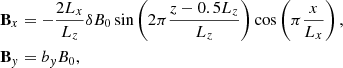

where dcs is the half thickness of RCS. The B0y is the initial guiding field, which is perpendicular to the reconnection plane. We compared the results with bg = B0y/B0z = 0 and 1.
The initial reconnection electric field Estatic, induced by the ambient particles dragged into a diffusion region with velocity Vinflow by a reconnection process, is assumed to be constant, both inside the reconnecting region and outside it. This electric field is thus perpendicular to the current sheet (x − z plane):
where the max amplitude of E0 is calculated from the plasma inflow into the RCS: E0 = VinflowB0.
2.2. Plasma feedback
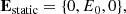
The electromagnetic fields inside current sheets E and B have two components: a background one (Estatic and Bstatic), described in Sect. 2.1, and a local component ( and
and  ), induced on a kinetic scale by accelerated particles. Hence, the total electromagnetic fields inside a current sheet are defined as
  and
and  .
.
The electric and magnetic fields induced by accelerated particles are calculated with Maxwell’s equations as follows:
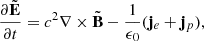
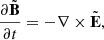
where je and jp are the current densities of electrons and protons updated by the particle solver. Maxwell’s equations are solved numerically via a standard finite-difference time-domain (FDTD) method.
2.3. Accepted parameters
The initial ambient density profile in a current sheet is described as follows:
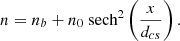
The simulations were performed with a mass ratio mi/me = 100, a background plasma density nb/n0 = 0.2, a frequency ratio ωpe/Ωce = 1.5, and dcs = 0.5di, where di is the ion inertial length. The temperature ratio Ti/Te is tested with 5 (the geomagnetic tail) and 1 (the solar wind environment) for comparison. The simulation domain was Lx × Lz = 51.2di × 12.8di, using 2048 × 512 cells and 100 particles per cell. The periodic boundary conditions were applied to both the electromagnetic field and particles along the z and y directions. Along the x direction, the conducting boundary condition for the electromagnetic field and the open boundary condition for particles were used. The simulations were generally run over a long time,  , where Ωci is the ion cyclotron frequency.
2.4. Simulation of current sheets with magnetic islands
Magnetic reconnection was triggered by a small distortion in Bz, δB0, at the beginning of the simulation:
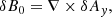
where
which satisfies the conditions:
The distortion initiates a fast reconnection that occurs near the centre of the simulation box shown in Fig. 1. Due to the periodic boundary condition at both ends of the z-axis, the simulation domain at later times represents the RCSs with a chain of magnetic islands; this is different from previous studies that used a single X-nullpoint geometry with open exhausts (Xia & Zharkova 2020).
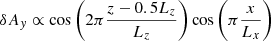
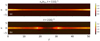 |
Fig. 1. Energy distributions of electrons on the x − z plane at (a) |


3. Simulation results
3.1. General comments on particle acceleration in a 3D RCS
3.1.1. Charge separation effect
In a 3D current sheet with a single X-nullpoint, the neutral ambient plasma is dragged into the diffusion region, where magnetic field reconnection occurs. Proton and electrons become drifting in the same direction along the current sheet midplane from the X-nullpoint towards the current sheet exhaust, while being accelerated by a reconnection electric field (Zharkova & Gordovskyy 2004; Zharkova et al. 2011; Xia & Zharkova 2018). Particles are then ejected from the RCS when they gain the critical energy required for them to break from a given magnetic field topology (Zharkova & Agapitov 2009). Because in a magnetic field accelerated protons and electrons also gyrate in opposite directions, they get ejected into the opposite semi-planes from the current sheet midplane in 3D magnetic topologies with a guiding field (Zharkova & Gordovskyy 2004; Pritchett & Coroniti 2004). However, the particle separation becomes partial or even negligible if the guiding field is weak (Zharkova & Gordovskyy 2005).
It should be noted that Zharkova & Gordovskyy (2004) provided the analytical solution of the motion equations in 3D magnetic topologies, explaining this charge separation between electrons and protons (ions), the tangential velocity Vx, and the ejection positions of the particle s ∝(qs/ms)1/3 (see the Eq. (8) in Sect. 3.1 in Zharkova & Gordovskyy 2004). Therefore, for a given 3D magnetic field topology with a guiding field, the electrons (with a negative charge) can be ejected from the midplane (X = 0) into the positive side (X > 0), while protons (with a positive charge) should be ejected from the midplane into the negative side (X < 0). This charge separation has been confirmed by numerous other simulations (see, for example, review Zharkova et al. 2011 and references therein).
The first important consequence of different motions of electrons and protons in an RCS comes from the fact that electrons need much shorter drift lengths than protons to gain the critical energy (a few hundred metres vs. a few kilometres in the corona) (Zharkova & Agapitov 2009). In the flare current sheet, the electrons are first ejected from the RCS and then try to ‘run away’ from an RCS into a magnetic loop. However, they are returned by the electric field of the accelerating protons, which still reside in the midplane, thus forming an electron cloud around the current sheet located on a loop top (Siversky & Zharkova 2009), which is often seen in flares as hard X-ray coronal sources (Zharkova et al. 2011). These first escaping electrons can be the triggers of solar flare onsets or flare precursors, while the flare itself occurs after the protons reach the critical energy and break from the magnetic topology of the RCS, precipitating together with electrons into (either the same or opposite) magnetic loop legs (Zharkova & Gordovskyy 2004; Zharkova & Agapitov 2009).
The PIC simulations of particle acceleration in a low-density current sheet reproduce the similar results obtained from the test-particle simulations, showing the charge separation in the velocity phase space in the RCSs (Siversky & Zharkova 2009; Zharkova & Khabarova 2012). However, for higher ambient plasma density the accelerated particle density and energy distributions reveal noticeable differences relative to the test-particle approach, where the asymmetry of ejected protons and electrons is more distinguishable in the energy distributions rather than in the density distributions. This similar charge separation has recently been confirmed for current sheets with magnetic islands, using both the test-particle and PIC approaches (Xia & Zharkova 2018, 2020).
The second important consequence of different motions of electrons and protons in a 3D RCS is the induction of a polarization electric field, Ep, between these particles of opposite charges across the current sheet midplane. The Ep (which could only be derived from PIC simulations) is larger than the reconnection electric field by up to two orders of magnitude (see also Siversky & Zharkova 2009; Zharkova & Khabarova 2012; Xia & Zharkova 2020). The induced Ep is mainly perpendicular to the RCS midplane (Siversky & Zharkova 2009; Zharkova & Khabarova 2012) and is found to increase with higher ambient plasma density (Xia & Zharkova 2020). This Ep is shown to define the velocity profiles of ions in the heliosphere during their crossing of the HCSs, as shown in a comparison of the PIC simulations with the in situ observations of the ion velocity profiles (Zharkova & Khabarova 2012).
3.1.2. Transit versus bounced particles of the same charge
For the particles with the same charge, a distinction also exists if they enter the RCS from opposite boundaries (Siversky & Zharkova 2009; Zharkova et al. 2011). Particles that enter the RCS from the side opposite to the side from which they are ejected are classified as ‘transit’ particles. While the particles that enter the RCS from the same side where they are ejected become decelerated while reaching the midplane, are classified as ‘bounced’ particles. The transit particles gain energy from the moment they enter the RCS and move towards the midplane, while bounced particles lose their energy during their migration from the current sheet edge towards the midplane (Zharkova & Gordovskyy 2005). As a result, the transit particles gain much higher energies and form power-law energy spectra (Litvinenko 1996), while the bounced electrons gain much lower energies and often have quasi-thermal energy spectra (Zharkova & Gordovskyy 2005; Siversky & Zharkova 2009; Xia & Zharkova 2018, 2020).
Therefore, the electrons accelerated in the RCS are split into two distinct groups in energy: the low-energy bounced electrons and high-energy transit electrons. The threshold of the separation by energy is dependent on the magnetic field topology. The uneven spatial and energy distributions of transit and bounced particles across the midplane are easy to distinguish in the test-particle approach and are a bit smoother in the PIC approach (Siversky & Zharkova 2009; Xia & Zharkova 2018). As a result, the accelerated electrons and protons have bump-on-tail energy distributions, which naturally triggers plasma turbulence due to Buneman instability (Buneman 1958).
Moreover, the asymmetry between the transit and bounced particles is also identified in the PADs. The corresponding PADs in higher-energy (transit particles) and lower-energy (bounced particles) channels were explored near a single X-nullpoint of the HCS, which showed bounced electrons turning from the current sheet at some distance away from the midplane (Zharkova & Khabarova 2012). The preliminary results for PADs in RCSs with a few magnetic islands exhibited a bi-directionality of the transit electron PADs in the higher-energy channel when the satellites (or virtual observer) moves across the magnetic island (Khabarova et al. 2020).
This opens up a new perspective to analyse in more detail the PADs of electrons (proton PADs are less accessible) accelerated in RCSs with and without magnetic islands using different physics parameters in space, which can be observed when a virtual spacecraft crosses these areas in different directions. The results can benchmark some in situ observations recorded by real spacecraft crossing similar structures in the heliosphere.
3.2. Electron PADs in the vicinity of a single X-nullpoint
In the current research, we started by exploring the electron PADs in a 3D RCS with a single X-nullpoint as an illustration. When the reconnection starts or when magnetic islands are formed, we have assumed that a spacecraft (we call it a ‘hypothetical spacecraft’ or ‘virtual spacecraft’) moves straight across the RCS at different locations and different angles, such as the vertical green line perpendicular to the RCS midplane in Fig. 2(P). The virtual spacecraft records the data of electron PADs on its way. Since accelerated electrons would have both transit and bounced particles with high and low energies as explained in Sect. 3.1.2, we split the PADs into higher-energy and lower-energy channels. This split was motivated by the channels usually present in the satellite payload for electron observations in the solar wind (e.g., the electron analyser SPAN-E of the SWEA instrument on the Parker Solar Probe covers 32 energy bands from 2 eV to 1.8+ keV) (Kasper et al. 2019).
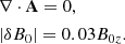
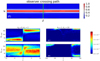 |
Fig. 2. PADs of electrons observed when a hypothetical spacecraft crosses an RCS with a single X-nullpoint. The top panel (P) shows that the sampled crossing path of the spacecraft is perpendicular to the RCS midplane (solid green line). The in-plane magnetic field topology is drawn with black lines with the amplitudes of By (bg = 1 case) indicated by the background colours. The PADs of high-energy electrons (second row) and lower-energy electrons (third row) obtained from panel a0 are presented in panels a1 and a2. The PADs shown in panels b1 and b2 are recorded along the same path as in panels a1 and a2 when the virtual spacecraft crosses an RCS with no guiding field (bg = 1). |
Without any guiding field (bg = 0) in the single X-nullpoint scenario, the electron PADs in all energy channels are symmetric with respect to the reconnection midplane x = 0 in Fig. 2(a1, a2) because the magnetic field does not impose any separation by charge, and no transit or bounced particles formed. Some electrons dragged into the RCS are accelerated to higher energies. They form high-energy beams and are ejected away from the X-nullpoint. Therefore, their pitch angles range from (10 ± 10)° at x < 0 to (170 ± 10)° at x > 0 (the sign changes because the Bx sign is reversed across the midplane) in panel a1. The other electrons gain less energy and form a wide range of pitch angles in panel a2; they thus have a nearly homogeneous distribution and join the ambient plasma electrons already present inside the RCS.
If the guiding field is strong, the PADs become strongly asymmetric across the midplane. For example, only the electrons with pitch angles of 180° are featured in the simulation performed for a thicker current sheet (dcs = 10), and bg = 1, as shown in Fig. 2(b1, b2). It is evident that when the guiding field becomes stronger, the transit electrons with higher energies and narrower pitch angle dispersion (175 ± 5)° become dominant in the opposite semi-plane (the right part in Fig. 2(b1)). This emphasizes a preferential direction of motion for higher-energy electrons since they represent the transit particles, which gain more energy (Litvinenko 1996; Zharkova & Gordovskyy 2005; Siversky & Zharkova 2009, see Sect. 3.1.2).
On the other hand, the counter-streaming (bounced) electrons appear in the lower-energy channel that shows the electrons entering the RCS at the pitch angle of (0 ± 15)° at X > 0 and approaching the distance of 50 ρi; they are ejected at the pitch angles of (160 ± 20)°. This results in energy dropouts for the bounced lower-energy electrons around the midplane as shown in Fig. 2(b2), which is often recorded in the in situ observations (Khabarova et al. 2020). The lower-energy electrons at X < 0 include bounced particles and those entering the current sheet that will move into the well-directed high-energy beam ejected at X>0 that is shown in Fig. 2(b1).
3.3. Electron PADs in magnetic islands
The magnetic field topology is more complicated in magnetic islands. The simulation described in Sect. 2 formed small magnetic islands that later merged into a large island located across the periodic boundary, which is similar to other simulations done by Drake et al. (2006) and Daughton et al. (2011). Owing to the periodic boundary condition at both ends of the z-axis, the simulation domain represents the RCSs with a chain of magnetic islands. This is different from previous studies carried out for a single X-nullpoint topology with open exhausts or with a chain of coalescent and squashed magnetic islands (Xia & Zharkova 2020). We investigated the two cases of magnetic field topologies: those with weak guiding fields and those with strong guiding fields.
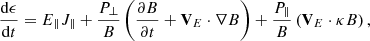
We have assumed that the virtual spacecraft crosses the simulation domain at different angles along the directions shown in Figs. 3 (for a weak guiding field) and 4 (for a strong guiding field). The most compelling regions including the vicinity of X-nullpoints, the midplane, and the magnetic island edges, are inspected by several paths, which are shown by the thick green lines.
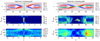 |
Fig. 3. PADs observed when a hypothetical spacecraft crosses an RCS at different angles at t = 33Ωi. Left column: path perpendicular to the midplane x = 0. Right column: path quasi-parallel to the midplane. The color bars in the top rows indicate the amplitudes of generated By with the in-plane magnetic field topology (black lines) and the paths of the spacecraft (green lines). The middle and bottom rows present the PADs of higher- and lower-energy electrons seen on the paths. The simulation starts with no guiding field (bg = 0). |
The energy threshold, ϵthreshold, between the higher- and lower-energy bands enabled us to distinguish the different PADs induced by transit and bounced particles. Based on the selected parameters described in Sect. 2, we found ϵthreshold = 9.67ϵth, where ϵth is the initial thermal energy. We started with Ti/Te = 5 as there are numerous observations with such thresholds reported from the Magnetospheric Multiscale Mission (MMS; Øieroset et al. 2002; Huang et al. 2016; Oka et al. 2016).
3.3.1. Weak guiding field
If the virtual spacecraft vertically crosses the X-nullpoint regarding the reconnecting midplane (left column of Fig. 3), it records the high-energy electrons with wide PADs peaking near 90° within the narrow region ≤0.5di near the midplane (a2). There are some weak signs of bi-directional beams with narrow PADs centred around 0° (bottom) and 180° (top). Meanwhile, the lower-energy electrons shown in panel a3 reflect the bidirectional beams clearly exiting in the range [ − 2, −0.25di] below and [0.25, 2di] above the X-nullpoint. When the crossing path is quasi-parallel to the midplane (right column of Fig. 3), the bi-directional beams in the higher-energy channel are more distinct in the islands (z = 0 − 12di and 40 − 51.2di), which are ∼14di away from the X-nullpoint in panel b2.
However, the edges of the magnetic island near the X-nullpoint still reveal the feature with the distinct PAD about 90° in the higher-energy channel. Different from the vertical path shown in panels a1 to a3, the counterpart of the bi-directional markings in the islands (b2) in the lower-energy channel shows nearly dispersionless vertical patterns (b3). Weak bi-directional strahls are also seen in the lower-energy channel at the exhausts of magnetic islands (towards the X-nullpoint).
To understand the obtained results, we used the findings of Xia & Zharkova (2020), who evaluated different energization terms for particle acceleration in RCSs with the guiding-centre drift approach (Drake et al. 2006; le Roux et al. 2015). The energy change of particle s mainly comes from:
where ϵ is the total kinetic energy of the particles of the same species. The first term on the right-hand side counts for the contribution from the parallel electric field, E∥, and J∥ stands for the parallel current. The second term corresponds to Betatron acceleration, which is linked to magnetic field compression or expansion. The third term describes curvature-drift (Fermi-type) acceleration, where the curvature κ = b ⋅ ∇b, with b the unit vector along B, and P⊥, P∥ are the parallel and perpendicular pressures. Previous results have shown that the contribution from E∥J∥ is much smaller than those of the other two terms (Dahlin et al. 2017; Xia & Zharkova 2020).
From the current results in Fig. 3(b3), we can deduce that lower-energy (bounced) electrons are scattered in the magnetic island with wide PADs. While the transit electrons follow the magnetic field line curvature and gain their energy from X-nullpoints on both sides of the island (Xia & Zharkova 2018), which is due to the first-order Fermi-type acceleration. Thus, the pitch angles of the transit electrons would have PADs directed along 0° /180° in panels a2 and b2, extending from the exhausts into the magnetic islands. Meanwhile, the beams directed around 90° are located near the X-nullpoint in panels a3, and b3, which is consistent with strong magnetic field relaxation in this region.
3.3.2. Strong guiding field
When the guiding field is strong (e.g., bg = 1 in Fig. 4), it reduces the compressibility of the magnetic field, while keeping particles longer within a given magnetic topology. Thus, the 90° beams disappear from the location close to the X-nullpoint and Fermi-type curvature-drift acceleration becomes dominant.
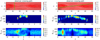 |
Fig. 4. PADs observed by a virtual spacecraft in the simulation starting with a strong guiding field (bg = 1) at t = 33Ωi. Left column: path perpendicular to the midplane x = 0. Right column: path across the separatrices. The magnetic field and the paths of the spacecraft (green lines) are demonstrated in the top row. The middle and bottom rows present the PADs of higher- and lower-energy electrons observed on the paths. |
We also notice that it is harder to observe bi-directional strahls during particle acceleration in this magnetic topology. The only region where the spacecraft observed counter-streaming beams was in the exhaust, between δz = 4 ∼ 9 away from the X-nullpoint at the end of the magnetic island, in the lower-energy channel shown in Fig. 4(a3). On the other hand, the strahl is near 180° at the X-nullpoint. It shifts towards 90° as the spacecraft moves close to the separatrices in the higher-energy channel of Fig. 4(a2).
We re-ran the simulation with ambient particle temperature ratio Ti/Te = 1, which is more common in the solar wind. It produced similar features as the Ti/Te = 5 case, such as the bi-directional strahls in a narrow region of the exhaust for bg = 1 and their existence around the X-nullpoint for the bg = 0 case. The main change of the electron PADs in the magnetic islands is shown in Fig. 5. As for the same threshold, the bi-directional signals are obscure in the higher-energy channel. The damping of the signals in the islands could be due to the larger gyroradius of electrons as Te increases from 1/5Ti to Ti.
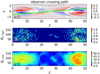 |
Fig. 5. PADs observed by a virtual spacecraft in the simulation starting with no guiding field (bg = 0) at t = 33Ωi. The path is quasi-parallel to the midplane (the angle between the path and the midplane is 3°). The initial temperature ratio Ti/Te = 1. |
Therefore, one can see that the observability of either the counter-streaming strahls or the heat-flux dropouts is highly dependent on the magnetic field topology and the crossing paths of real spacecraft. If a spacecraft can only access regions far from the X-nullpoint, it is likely to pick up the mono-directional strahl of high-energy electron beams. Energetic particles fly diagonally away from the main X-nullpoint when the guiding field is strong, while lower-energy electrons are recorded well before the current sheet crossing (Xia & Zharkova 2020). However, if the spacecraft passes across the current sheet with magnetic islands in different directions, as explored in this paper, different patterns of PADs are formed. They uniquely reflect the magnetic field topological specifics and the angle under which this reconnection site is observed. This can be a very useful tool for diagnostics of physical conditions of the environment producing the energetic particles.
4. Comparison with in situ observations
4.1. Observations with previous space missions
In this paper we explore the relationship between electron PADs and the magnetic topologies in 3D RCSs. Obviously, real spacecraft trajectories would not cross the RCSs in straight lines as considered in Figs. 2–4. However, the presented simulations can shed some light on different PAD features formed by energetic particles while spacecraft pass certain regimes of RCSs. In this subsection we present some evidence previously recorded by different missions near the Earth.
Our previous PIC simulations of particle acceleration near a single X-nullpoint for 3D magnetic topologies with strong guiding fields (Xia & Zharkova 2020) have shown the appearance of counter-streaming high-energy electrons diagonal from the X-nullpoint, formed by transit particles, on the one hand, and lower-energy electrons, formed by bounced particles, located inside and away from the X-nullpoints, on the other hand. In the observations, the WIND spacecraft at 1 AU recorded the U-shape (horseshoe-like) PADs of low-energy (bounced) electrons near the HCS (Zharkova & Khabarova 2012), similar to those shown in Fig. 2(b2). The electron strahls observed with WIND and STEREO in multiple magnetic islands in the heliosphere are also consistent with our current PIC simulations of energetic electron acceleration in RCSs with a chain of magnetic islands and their ejection from exhausts at both ends of the chain (Xia & Zharkova 2020).
For example, the electron PADS obtained in recent simulations of coalescent and squashed magnetic islands in 3D RCSs for a weak guiding field, bg = 0.1, showed that the bi-directional strahls can be complemented with the heat-flux dropout (low-energy electrons) seen inside magnetic islands (see Fig. 2, WIND data between 00 : 00 : 00 − 08 : 00 : 00, 2007-May-29 in Khabarova et al. 2020 for rapid changes of electron PADs in the current sheets with magnetic islands).
Such field-aligned bi-directional jets of high-energy electrons have also been reported: in the magnetotail (Fujimoto et al. 1997; Øieroset et al. 2002; Egedal et al. 2005; Pritchett 2006; Manapat et al. 2006; Oka et al. 2016); in the current sheets of a heliosphere (McComas et al. 1989; Foullon et al. 2009; Rouillard et al. 2010), where a strong guiding magnetic field is not a surprise; and at the font of an ICME (Zank et al. 2015), where strahls are moving perpendicular to the IMF but parallel to the magnetic field of the ICME current sheet. Furthermore, bi-directional electron beams in the lower-energy channels have also been found at the edge of a magnetic island (Huang et al. 2016).
On the other hand, the PADs of energetic electrons centred about 90° have been associated with trapped and mildly accelerated electrons in magnetic islands (Fu et al. 2013; Yao et al. 2018; Wang et al. 2019). These in situ measurements are consistent with our findings in Fig. 4(b2, b3). The THEMIS mission also reported similar PADs when it crossed the reconnection diffusion region of the magnetotail (Oka et al. 2016), such as the quasi-perpendicular (90°) and bi-directional distributions.
The detailed study in this paper shows that ∼90° strahls accumulate near the X-nullpoint at the end of magnetic islands when bg = 0 and shift into the magnetic islands when bg is large. Hence, the simulation in Fig. 3(b2, b3) suggests that WIND was travelling across a magnetic island pool with a strong guiding field.
Therefore, observers can distinguish whether the spacecraft was passing single or multiple O- and X-nullpoints in these current sheets by evaluating electron PADs and distinguishing between those moving in quasi-parallel and quasi-perpendicular directions.
4.2. New observations with Parker Solar Probe
Most recently, during Perihelion 1 of PSP, 21 RCSs were identified by the paired rotational discontinuities bounding the exhausts (Phan et al. 2020). However, due to the low resolution (≥27s) of the spacecraft PAD measurement at this moment, PSP could only sample zero to four times in the RCS, and could only record < 2 samples during the surveyed time. Still, we were able to identify two events (IDs 7 and 15 in the table in Phan et al. 2020) that show the electron PAD patterns near a single X-nullpoint.
The PADs in different energy bands and the change of magnetic field components are shown in Fig. 6(a1, a2). The period of the first RCS crossing was 65.7s, and the guiding field was weak (0.82 nT). The electron beam streaming from the Sun (Kasper et al. 2019) was locally discontinued. The reversing of the mono-directional strahls from 180° to 0° across the RCS was presented in the higher-energy channels, > 253 eV, which is consistent with Fig. 2(a1).
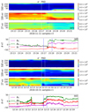 |
Fig. 6. Electron PADs averaged over 253.3 − 934.2, 55 − 164.6, and 9.7 − 44.3 channels from top to bottom. The left and right columns come from two different events. The bottom panels show the magnetic field components in the RTN coordinate. The vertical dashed lines mark the crossing of the RCS. |
The second case is presented in Fig. 6(b1, b2). It shows a heat-flux dropout in the higher-energy channel (> 55 eV). The mono-directional strahl at 180° could be a combination of local accelerated electrons and the electron beams from the Sun. Meanwhile, the transition from mono-directional beams to bi-directional beams in the lower-energy channel (< 45 eV) matches rather closely with the features of PADs presented in Fig. 2(b2). Since the observed guiding field was rather weak (0.89 nT), and the simulation in Fig. 2(b) was made for a stronger guiding field, this good fit is likely caused by an increase in the current sheet width to 100ρi, for which the previous single X-nullpoint simulation was carried out.
We wish to further emphasize that the energy threshold for lower- and higher-energy electrons, when their PADs become qualitatively different, is ∼50 eV. This is smaller than the value of ≥100 eV obtained from the measurements near 1 AU in the solar wind (Khabarova et al. 2020), which suggests that the reconnection event in the RCS measured by PSP was weaker.
5. Conclusion
In the current paper, we studied the electron PADs in different parts of the magnetic islands during the magnetic reconnection. Our self-consistent PIC simulations considered the 3D reconnection models with a strong or weak magnetic guiding field and different electron-to-proton temperature ratios. Furthermore, we collected the electron PADs along the paths of the virtual spacecraft in different directions through the simulation regions, which can emulate real in situ observations. This is a supplement to the previous studies that considered the RCSs with either a single X-nullpoint geometry or a few coalescent and squashed magnetic islands (Xia & Zharkova 2020).
To understand the simulation results, we first reiterate the two key properties of particle acceleration in 3D RCSs with a single X-nullpoint: (1) separation of protons and ions from electrons with respect to the current sheet midplane if Bg > 0 and (2) different motions of transit and bounced particles (depending on which edge of the RCS they enter) within the same species. These properties introduce asymmetry in the particle energy distributions and PADs across the RCS midplane.
As shown in the previous study (Xia & Zharkova 2020), the transit particles in an RCS with a single X-nullpoint are ejected as high-energy strahls with rather narrow pitch angles centred around 0° or 180°, depending on which side of the X-nullpoint they are. On the contrary, the bounced electrons gain much less energy because they cannot reach the current sheet midplane where strong particle acceleration occurs. They have wide PADs centred in a direction that is dependent on the ratio of the magnetic field components. These two populations of energetic electrons are well distinguished in the models and can easily be detected from in situ observations. We have identified two RCSs in the most recent PSP database that show PAD features in the vicinity of a single X-nullpoint. We expect the high cadence data from Solar Orbiter to provide more insight into the RCS structures. That will help us carry out a further comparison our predictions and electron PADs closer to the Sun.
Although the parameters of the energy spectra and PADs change accordingly in magnetic islands, the asymmetry ejection is still present when the particles are ejected from the exhausts (Xia & Zharkova 2018). For example, when the magnetic guiding field is weak, it is easy for spacecraft to observe bi-directional strahls: The signals cover a wide range in the magnetic islands in the higher-energy channel due to the counter-streaming energetic electrons coming from the two X-nullpoints at both ends of the magnetic islands. A comparison of electron PADs in the simulations with different Ti/Te suggests that it is harder to capture the bi-directional beams inside the islands in the solar wind than in the geomagnetic tail environment due to the higher electron temperature. We also notice that the bi-directional strahls are complemented with the heat flux dropout (low-energy electrons) seen inside magnetic islands (Khabarova et al. 2020). Such field-aligned bi-directional strahls of high-energy electrons have been observed by many instruments in the current sheets of the magnetotail (Øieroset et al. 2002; Egedal et al. 2005; Pritchett 2006; Manapat et al. 2006; Oka et al. 2016), the current sheets of the heliosphere (WIND, THEMIS; McComas et al. 1989; Foullon et al. 2009; Rouillard et al. 2010), and at the font of ICMEs (STEREO; Zank et al. 2015).
The implementation of a strong guiding magnetic field in this model provides significant changes to electron PADs. The bi-directional strahls only exist in the exhaust region in the lower-energy channel, similar to the previous findings near a single X-nullpoint (Xia & Zharkova 2020). The counter-streaming energetic beam from another X-nullpoint is strongly suppressed by the guiding field. Nevertheless, bi-directional signals are accessible in the lower-energy channels in the exhausts for both Ti/Te = 1 and 5, with or without a strong guiding field. This signal has been detected in many observations (McComas et al. 1989; Crooker et al. 2003; Pagel et al. 2005; Rouillard et al. 2010; Simunac et al. 2012; Huang et al. 2016).
The PADs in higher-energy channels rotate from quasi-parallel (near the X-nullpoint) to quasi-perpendicular (in the magnetic island away from the X-nullpoint), depending strongly on the crossing path in the simulation domain. In fact, the PADs of energetic electrons are centred at ∼90°, as observed in some cases (Fu et al. 2013; Yao et al. 2018; Wang et al. 2019). The detailed study in this paper shows that ∼90° strahls are located near the X-nullpoint at the end of magnetic islands when the guiding field is weak, and they shift inside the magnetic islands when the guiding field becomes strong. These findings regarding electron PADs, in addition to their energy distributions, can be a diagnostic tool that can help to explain a whole range of the disperse electron PAD observations from near the Earth to the inner heliosphere.
Acknowledgments
The authors wish to thank the anonymous referee for useful and constructive comments, from which the paper strongly benefited. The authors acknowledge the funding for this research provided by the US Air Force grant PRJ02156. This work used the DiRAC Complexity system, operated by the University of Leicester IT Services, which forms part of the STFC DiRAC HPC Facility (www.dirac.ac.uk). This equipment is funded by BIS National E-Infrastructure capital grant ST/K000373/1 and STFC DiRAC Operations grant ST/K0003259/1. DiRAC is part of the National e-Infrastructure.
References
- Anderson, B. R., Skoug, R. M., Steinberg, J. T., & McComas, D. J. 2012, J. Geophys. Res., 117, A04107 [Google Scholar]
- Bowers, K. J., Albright, B. J., Yin, L., Bergen, B., & Kwan, T. J. T. 2008, Phys. Plasma, 15 [Google Scholar]
- Buneman, O. 1958, Phys. Rev. Lett., 1, 8 [Google Scholar]
- Cerutti, B., Werner, G. R., Uzdensky, D. A., & Begelman, M. C. 2013, ApJ, 770, 147 [Google Scholar]
- Chian, A. C. L., & Muñoz, P. A. 2011, ApJ, 733, L34 [Google Scholar]
- Crooker, N. U., & Pagel, C. 2008, J. Geophys. Res., 113, A02106 [Google Scholar]
- Crooker, N. U., Larson, D. E., Kahler, S. W., Lamassa, S. M., & Spence, H. E. 2003, Geophys. Res. Lett., 30, 1619 [Google Scholar]
- Crooker, N. U., Huang, C.-L., Lamassa, S. M., et al. 2004, J. Geophys. Res., 109, 170 [Google Scholar]
- Dahlin, J. T., Drake, J. F., & Swisdak, M. 2017, Phys. Plasmas, 24, 092110 [Google Scholar]
- Daughton, W., Roytershteyn, V., Karimabadi, H., et al. 2011, Nat. Phys., 7, 539 [Google Scholar]
- de Gouveia dal Pino, E. M., & Lazarian, A. 2005, A&A, 441, 845 [NASA ADS] [CrossRef] [EDP Sciences] [Google Scholar]
- Drake, J. F., Swisdak, M., Schoeffler, K. M., Rogers, B. N., & Kobayashi, S. 2006, Geophys. Res. Lett., 33, L13105 [Google Scholar]
- Drake, J. F., Cassak, P. A., Shay, M. A., Swisdak, M., & Quataert, E. 2009, ApJ., 700, L16 [Google Scholar]
- Egedal, J., Øieroset, M., Fox, W., & Lin, R. P. 2005, Phys. Rev. Lett., 94, 025006 [Google Scholar]
- Eyink, G. L. 2015, ApJ, 807, 137 [Google Scholar]
- Feuerstein, W. M., Larson, D. E., Luhmann, J. G., et al. 2004, Geophys. Res. Lett., 31, L22805 [Google Scholar]
- Foullon, C., Lavraud, B., Wardle, N. C., et al. 2009, Sol. Phys., 259, 389 [Google Scholar]
- Fu, H. S., Khotyaintsev, Y. V., Vaivads, A., Retinò, A., & André, M. 2013, Nat. Phys., 9, 426 [Google Scholar]
- Fujimoto, M., Nakamura, M. S., Shinohara, I., et al. 1997, Geophys. Res. Lett., 24, 2893 [Google Scholar]
- Gosling, J. T., Baker, D. N., Bame, S. J., et al. 1987, J. Geophys. Res., 92, 8519 [Google Scholar]
- Gosling, J. T., Eriksson, S., & Schwenn, R. 2006, J. Geophys. Res., 111, A10102 [Google Scholar]
- Graham, G. A., Rae, I. J., Owen, C. J., et al. 2017, J. Geophys. Res., 122, 3858 [Google Scholar]
- Guo, F., Li, H., Daughton, W., & Liu, Y.-H. 2014, Phys. Rev. Lett., 113, 155005 [Google Scholar]
- Horaites, K., Boldyrev, S., & Medvedev, M. V. 2018, MNRAS, 484, 2474 [Google Scholar]
- Huang, Y.-M., & Bhattacharjee, A. 2010, Phys. Plasmas, 17, 062104 [Google Scholar]
- Huang, S. Y., Sahraoui, F., Retino, A., et al. 2016, Geophys. Res. Lett., 43, 7850 [Google Scholar]
- Hurford, G. J., Krucker, S., Lin, R. P., et al. 2006, ApJ, 644, L93 [Google Scholar]
- Kahler, S. W., & Lin, R. P. 1995, Sol. Phys., 161, 183 [Google Scholar]
- Kajdič, P., Blanco-Cano, X., Opitz, A., et al. 2013, AIP Conf. Proc., 1539, 203 [Google Scholar]
- Karimabadi, H., Dorelli, J., Roytershteyn, V., Daughton, W., & Chacón, L. 2011, Phys. Rev. Lett., 107, 025002 [Google Scholar]
- Kasper, J. C., Bale, S. D., Belcher, J. W., et al. 2019, Nature, 576, 228 [Google Scholar]
- Khabarova, O., Zharkova, V., Xia, Q., & Malandraki, O. E. 2020, ApJ, 894, L12 [Google Scholar]
- Lapenta, G., Markidis, S., Goldman, M. V., & Newman, D. L. 2015, Nat. Phys., 11, 690 [Google Scholar]
- Lazarian, A., Vlahos, L., Kowal, G., et al. 2012, Space Sci. Rev., 173, 557 [Google Scholar]
- le Roux, J. A., Zank, G. P., Webb, G. M., & Khabarova, O. 2015, ApJ, 801, 112 [Google Scholar]
- le Roux, J. A., Zank, G. P., Webb, G. M., & Khabarova, O. V. 2016, ApJ, 827, 47 [Google Scholar]
- le Roux, J. A., Zank, G. P., & Khabarova, O. V. 2018, ApJ, 864, 158 [Google Scholar]
- Li, X., Guo, F., Li, H., Stanier, A., & Kilian, P. 2019, ApJ, 884, 118 [Google Scholar]
- Litvinenko, Y. E. 1996, ApJ, 462, 997 [Google Scholar]
- Loureiro, N. F., Cowley, S. C., Dorland, W. D., Haines, M. G., & Schekochihin, A. A. 2005, Phys. Rev. Lett., 95 [Google Scholar]
- Manapat, M., Øieroset, M., Phan, T. D., Lin, R. P., & Fujimoto, M. 2006, Geophys. Res. Lett., 33, L05101 [Google Scholar]
- Markidis, S., Lapenta, G., Divin, A., et al. 2012, Phys. Plasmas, 19, 032119 [Google Scholar]
- Matthaeus, W. H., Ambrosiano, J. J., & Goldstein, M. L. 1984, Phys. Rev. Lett., 53, 1449 [Google Scholar]
- McComas, D. J., Gosling, J. T., Phillips, J. L., et al. 1989, J. Geophys. Res., 94, 6907 [Google Scholar]
- Muñoz, P. A., & Büchner, J. 2016, Phys. Plasmas, 23, 102103 [Google Scholar]
- Nishizuka, N., & Shibata, K. 2013, Phys. Rev. Lett., 110, 051101 [Google Scholar]
- Øieroset, M., Lin, R. P., Phan, T. D., Larson, D. E., & Bale, S. D. 2002, Phys. Rev. Lett., 89 [Google Scholar]
- Oka, M., Phan, T.-D., Krucker, S., Fujimoto, M., & Shinohara, I. 2010, ApJ, 714, 915 [Google Scholar]
- Oka, M., Phan, T.-D., Øieroset, M., & Angelopoulos, V. 2016, J. Geophys. Res., 121, 1955 [Google Scholar]
- Pagel, C., Crooker, N. U., Larson, D. E., Kahler, S. W., & Owens, M. J. 2005, J. Geophys. Res., 110, A01103 [Google Scholar]
- Phan, T. D., Bale, S. D., Eastwood, J. P., et al. 2020, ApJS, 246, 34 [Google Scholar]
- Pritchett, P. L. 2006, J. Geophys. Res., 111, A10212 [Google Scholar]
- Pritchett, P. L., & Coroniti, F. V. 2004, J. Geophys. Res., 109, A01220 [Google Scholar]
- Rouillard, A. P., Lavraud, B., Davies, J. A., et al. 2010, J. Geophys. Res., 115, A04104 [Google Scholar]
- Roux, J. A. L., Webb, G. M., Khabarova, O. V., Zhao, L.-L., & Adhikari, L. 2019, ApJ, 887, 77 [Google Scholar]
- Sauvaud, J. A., Larson, D., Aoustin, C., et al. 2008, Space Sci. Rev., 136, 227 [Google Scholar]
- Simunac, K. D. C., Galvin, A. B., Farrugia, C. J., et al. 2012, Sol. Phys., 281, 423 [Google Scholar]
- Siversky, T. V., & Zharkova, V. V. 2009, J. Plasma Phys., 75, 619 [Google Scholar]
- Verboncoeur, J. P., Langdon, A. B., & Gladd, N. T. 1995, Computer Physics Communications, 87, 199 [Google Scholar]
- Vocks, C., Salem, C., Lin, R. P., & Mann, G. 2005, ApJ, 627, 540 [Google Scholar]
- Štverák, Š., Maksimovic, M., Trávníček, P. M., et al. 2009, J. Geophys. Res., 114, A05104 [Google Scholar]
- Wang, S., Wang, R., Yao, S. T., et al. 2019, J. Geophys. Res., 124, 1753 [Google Scholar]
- Xia, Q., & Zharkova, V. 2018, A&A, 620, A121 [NASA ADS] [CrossRef] [EDP Sciences] [Google Scholar]
- Xia, Q., & Zharkova, V. 2020, A&A, 635, A116 [EDP Sciences] [Google Scholar]
- Yao, S. T., Shi, Q. Q., Liu, J., et al. 2018, J. Geophys. Res., 123, 5561 [Google Scholar]
- Zank, G. P., Hunana, P., Mostafavi, P., et al. 2015, ApJ, 814, 137 [Google Scholar]
- Zenitani, S., & Hoshino, M. 2008, ApJ, 677, 530 [Google Scholar]
- Zhang, S., Du, A. M., Feng, X., et al. 2014, Sol. Phys., 289, 1607 [Google Scholar]
- Zharkova, V. V., & Agapitov, O. V. 2009, J. Plasma Phys., 75, 159 [Google Scholar]
- Zharkova, V. V., & Gordovskyy, M. 2004, ApJ, 604, 884 [Google Scholar]
- Zharkova, V. V., & Gordovskyy, M. 2005, MNRAS, 356, 1107 [Google Scholar]
- Zharkova, V. V., & Khabarova, O. V. 2012, ApJ, 752, 35 [Google Scholar]
- Zharkova, V., & Khabarova, O. 2015, Ann. Geophys., 33, 457 [Google Scholar]
- Zharkova, V. V., Arzner, K., Benz, A. O., et al. 2011, Space Sci. Rev., 159, 357 [Google Scholar]
- Zhong, J. Y., Lin, J., Li, Y. T., et al. 2016, Ap&SS, 225, 30 [Google Scholar]
All Figures
|
Fig. 1. Energy distributions of electrons on the x − z plane at (a) |
| In the text | |
|
Fig. 2. PADs of electrons observed when a hypothetical spacecraft crosses an RCS with a single X-nullpoint. The top panel (P) shows that the sampled crossing path of the spacecraft is perpendicular to the RCS midplane (solid green line). The in-plane magnetic field topology is drawn with black lines with the amplitudes of By (bg = 1 case) indicated by the background colours. The PADs of high-energy electrons (second row) and lower-energy electrons (third row) obtained from panel a0 are presented in panels a1 and a2. The PADs shown in panels b1 and b2 are recorded along the same path as in panels a1 and a2 when the virtual spacecraft crosses an RCS with no guiding field (bg = 1). |
| In the text | |
|
Fig. 3. PADs observed when a hypothetical spacecraft crosses an RCS at different angles at t = 33Ωi. Left column: path perpendicular to the midplane x = 0. Right column: path quasi-parallel to the midplane. The color bars in the top rows indicate the amplitudes of generated By with the in-plane magnetic field topology (black lines) and the paths of the spacecraft (green lines). The middle and bottom rows present the PADs of higher- and lower-energy electrons seen on the paths. The simulation starts with no guiding field (bg = 0). |
| In the text | |
|
Fig. 4. PADs observed by a virtual spacecraft in the simulation starting with a strong guiding field (bg = 1) at t = 33Ωi. Left column: path perpendicular to the midplane x = 0. Right column: path across the separatrices. The magnetic field and the paths of the spacecraft (green lines) are demonstrated in the top row. The middle and bottom rows present the PADs of higher- and lower-energy electrons observed on the paths. |
| In the text | |
|
Fig. 5. PADs observed by a virtual spacecraft in the simulation starting with no guiding field (bg = 0) at t = 33Ωi. The path is quasi-parallel to the midplane (the angle between the path and the midplane is 3°). The initial temperature ratio Ti/Te = 1. |
| In the text | |
|
Fig. 6. Electron PADs averaged over 253.3 − 934.2, 55 − 164.6, and 9.7 − 44.3 channels from top to bottom. The left and right columns come from two different events. The bottom panels show the magnetic field components in the RTN coordinate. The vertical dashed lines mark the crossing of the RCS. |
| In the text | |
Current usage metrics show cumulative count of Article Views (full-text article views including HTML views, PDF and ePub downloads, according to the available data) and Abstracts Views on Vision4Press platform.
Data correspond to usage on the plateform after 2015. The current usage metrics is available 48-96 hours after online publication and is updated daily on week days.
Initial download of the metrics may take a while.