© ESO 2020

1 Introduction

A dynamo is the magnetohydrodynamic (MHD) process that converts kinetic energy of fluid motions into electromagnetic energy (Jones 2014; Zhang & Schubert 2000). The intrinsic magnetic fields of celestial objects are believed to be generated and sustained by active dynamo processes (Christensen et al. 2008; Stanley & Glatzmaier 2009). To successfully drive a dynamo, thermal and compositional instabilities are typically the main power sources (Lister & Buffett 1995; Glatzmaier 2002). Other arguments have been made that mechanical forces associated with nonuniform rotation, such as precession and libration, can also energize dynamo (Wood 1966; Lagrange et al. 2011; Stefani et al. 2014). In our Solar System, an intrinsic planetary magnetic field is common for fast-rotating planets. Jupiter and Saturn belong to this class and have very strong and stable dipole-dominant fields (Dougherty et al. 2018; Moore et al. 2018). Understanding the powerful dynamo processes operating in gaseous planets is a well-recognized important and interesting open question in planetary physics.

In our Earth, the geodynamo operates in the fluid iron-nickel outer core (Buffett 2000). Various geophysical or geodetic observations are available to indirectly probe several key physical parameters of the geodynamo, such as electrical and thermal conductivity, heat flux, the core-mantle boundary flow speed, and the temporal variation of the magnetic field (Mandea et al. 2012; Pozzo et al. 2012). However, for gaseous planets, our knowledge of the deep dynamo process operating in the metallic hydrogen region is much more limited (Kong et al. 2019), mainly because it is more difficult to constrain the internal states of giant planets compared with what we know about our Earth. Gaseous planets are primarily made of hydrogen and helium, which results in internal states that differ sharply from the interiors of terrestrial planets, which are made of heavy elements (Stevenson 1982; Guillot 2005). The mysteries regarding the location, amplitude, and structure of the fluid motion of the Jovian or Saturnian deep convective dynamo are more numerous and deeper.

Several forward or inverse approaches have been tried in order to understand the Jovian or Saturnian dynamo. The Juno mission and the Cassini Grand Finale mission have revealed the detailed structures of the external magnetic fields outside the two planets (Connerney et al. 2018; Moore et al. 2018, 2019; Dougherty et al. 2018). However, direct measurements and inference of the morphology of the internal magnetic field of a gaseous planet is generally impossible. First, it is physically forbidden to extrapolate the outside potential field into the electrically conductive region. The stably stratified hydrogen-helium demixing layer between the dynamo region and the outer molecular hydrogen envelope (Morales et al. 2009; Militzer et al. 2016) is also believed to filter out and change the magnetic field that originates in the deeper dynamo region (Dougherty et al. 2018; Moore et al. 2018). Moreover, any toroidal component of the magnetic field existing in the dynamo region is entirely invisible to external observations. Forward simulations of the planetary dynamo are also difficult. Although progress has been made (Duarte et al. 2013; Jones 2014; Glatzmaier 2018), it is difficult to produce a numerical dynamo model that can exactly and comprehensively capture the highly complex and unknown dynamics. The essential problem is the huge gap between the numerically achievable parameter space and the real MHD parameters inside planets (Ogden et al. 2006; Christensen et al. 2008; Zhan et al. 2012; Jones 2014). By far, all inferences of dynamo of gaseous planets have been based on the internal states, which themselves are usually disputable or poorly constrained. As a result, it has long been an open problem to determine realistic properties of the dynamo processes operating inside gaseous planets.

With the aim to diagnose the deep convective dynamo of gaseous planets, Kong et al. (2016) first proposed gravity as a complementary way of probing the nonaxisymmetric structure of the deep convective dynamo through three-dimensional gravitational sounding. Kulowski et al. (2020) used a vorticity equation to estimate the axisymmetric distortions from possible zonal flows in the Jovian dynamo region, which are constructed according to Ferraro’s law of isorotation. The gravitational anomaly is caused by convective flow distortion. A gravitational signature can expose the dynamical structure of convection, especially asthe horizontal variation reflects the properties of the convective dynamo (Zhang & Jones 1996). If there is a large invisible toroidal component of the internal field in the deep dynamo region (Zhang & Jones 1994; Zhang 1995), for example, a small azimuthal wavenumber (large horizontal scale) dominating the structure of the fluid motion might be indicative of a strong-field dynamo. Conversely, a high value of the azimuthal wavenumber (small horizontal scale) might be indicative of a weak-field dynamo. This gravitational sounding technique is not about detecting temporal or secular variations of a planetary magnetic field, which has been done for Earth studies (Mandea et al. 2012; Pozzo et al. 2012).

The external gravitational field of a fast-rotating gaseous planet can be expanded by spherical harmonics in the spherical coordinates (r, θ, ϕ), whose origin is set to be at the center of mass, $$\begin{array}{l}{V}_{\text{g}}(r,\theta ,\varphi )=-\frac{GM}{r}[1-{\sum }_{n=2}^{\infty }{\left(\frac{R_S}{r}\right)}^n{\tilde{J}}_n{\tilde{P}}_n(\cos \theta )\\ -{\sum }_{n=2}^{\infty }{\sum }_{m=0}^n{\left(\frac{R_S}{r}\right)}^n{\tilde{C}}_{nm}{\tilde{P}}_{nm}(\cos \theta )\cos m\varphi \\ -{\sum }_{n=2}^{\infty }{\sum }_{m=0}^n{\left(\frac{R_S}{r}\right)}^n{\tilde{S}}_{nm}{\tilde{P}}_{nm}(\cos \theta )\sin m\varphi ], r\ge R_S,\end{array}$$(1)

in which G is the gravitational constant, M is the mass of the planet, R_S is the equatorial radius at the 1-bar level, ${\tilde{P}}_n$ are normalized Legendre polynomials, ${\tilde{P}}_{nm}$ are normalized associated Legendre polynomials, ${\tilde{J}}_n$ are zonal coefficients, and ${\tilde{C}}_{nm}$ and ${\tilde{S}}_{nm}$ are the tesseral and sectoral coefficients. The zonal gravitational harmonics are mainly contributed by the equilibrium structure under solid-body rotation, and contain axisymmetric gravitational distortions associated with zonal flows existing in the molecular hydrogen envelope (Hubbard 1999; Kong et al. 2014, 2018a; Kaspi et al. 2018). The tesseral and sectoral harmonics, representing nonaxisymmetric gravitational anomalies, are connected to nonaxisymmetric fluid motions; the convective dynamo flow is of interest in this paper. Although the azimuthal circulation in the molecular hydrogen envelope can be much stronger, its axisymmetric gravitational signature, which is contained in the zonal coefficients ${\tilde{J}}_n$, is distinctly different from nonaxisymmetric gravity, which is notated by the ${\tilde{C}}_{nm}$ and ${\tilde{S}}_{nm}$ coefficients, resulting from the convective dynamo flow in the metallic hydrogen region. Because of the natural split in gravitational spectrum, the nonaxisymmetric dynamo flow can be gravitationally separated from azimuthal circulations regardless of their relative strength.

Orbiting Saturn is the most efficient way to measure the gravitational field of Saturn. The study of the Saturnian gravity has a long history. A combined analysis of Pioneer 11 Doppler tracking and its satellite apse and node rate data yielded the first observational determination of the J₆ value of Saturn (Null et al. 1981). The harmonic coefficients J₂, J₄, and J₆ of Saturn calculated by Nicholson & Porco (1988) are consistent with the Pioneer 11 results. Campbell & Anderson (1989) analyzed the Doppler-tracking data and star-satellite imaging data from the Voyager 1 and Voyager 2 spacecrafts, combined with a reanalysis of the Pioneer 11 Doppler tracking. This yielded improved values of the Saturn gravitational harmonic coefficients up to the eighth zonal degree and accurate sectoral harmonic coefficients, C₂₂ and S₂₂. Furthermore, with the implementation of the Cassini mission, Jacobson et al. (2006) determined the gravity and mass of Saturn and its moons. The zonal gravitational coefficients of Saturn were also obtained to the eighth degree, while the uncertainty dropped sharply, by six times compared with the results of Campbell & Anderson (1989). Anderson & Schubert (2007) used Voyager andCassini tracking data to obtain the zonal gravitational coefficients up to the tenth degree. At the Grand Finale phase of the Cassini mission, the spacecraft dived between the planet and the innermost ring. The plunge reached down to 2600–3900 km above the cloud top of Saturn (Edgington & Spilker 2016). Iess et al. (2019) processed the tracking data obtained from five effective Grand Finale orbits and obtained 12-degree zonal gravitational coefficients. This solution is by far the most precise.

The Cassini Grand Finale mission reported a substantial nonaxisymmetric component of the gravitational field in order to explain the spacecraft orbit tracking data (Iess et al. 2019). There can be several sources of a Saturnian nonaxisymmetric gravitational field. Iess et al. (2019) tried incorporating the gravitational effects of tidal responses and normal modes into their precise orbit determination (POD) force model, but found it difficult to coherently account for any secular nonaxisymmetric gravitational field. We use POD simulations here to test whether the Cassini spacecraft actually sensed a dynamo-related nonaxisymmetric gravitational field. We have studied two possibilities,a strong-field and a weak-field dynamo, to examine the possibility of detecting the predicted gravitational signatures. Two questions are answered in this paper. First, whether the nonzonal gravitational field reported in Iess et al. (2019) is partly connected to the Saturnian convective dynamo, and second, which spacecraft mission configurations might detect the Saturnian dynamo. The latter question might be particularly useful for future relevant missions.

The paper is organized as follows. We present in Sect. 2 two types of convective dynamo flows that belong to two possible dynamo regimes and forward-compute their gravitational coefficients. Sections 3 and 4 present the answers to our two questions. A summary and perspectives are given in Sect. 5.

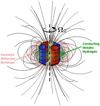Fig. 1 Sketch of a possible convective flow inside the metallic hydrogen-helium region of Saturn. The cylindrical pattern of fluid motions (∂u∕∂z = 0) reflects the fast-rotation effect (Zhang & Liao 2017), and the azimuthal number of columns indicates the typeof dynamo action (Zhang & Jones 1996). The flow has an azimuthal wave number 2, whichillustrates a possible convection of the strong-field dynamo (e.g., see Elsasser number Λ = 5.1 in Fig. 6 of Zhang 1995).

2 Gravitational signature of the Saturnian convective dynamo

In this section, the principle of gravitational sounding is discussed, conceptually following Kong et al. (2016). Figure 1 presents the schematics of a possible deep convective flow that exists in the metallic hydrogen region of Saturn. The parameterization of the fluid motion is adopted to mimic the dynamically possible structure of the convection under rotational and magnetic influence (Chandrasekhar 1962; Zhang & Schubert 2000).

Because we focus on gravitational sounding of the deep convective dynamo, we did not model other types of flow distortions from the semiconductive region, the molecular envelope, and the outer atmosphere. Because Saturn rotates very rapidly with the angular velocity $\widehat{z}{\Omega }_0$ and is in a statistically steady state, the Rossby number for the deep convective flow ${\mathcal{U}}_{0}u$ with the typical amplitude ${\mathcal{U}}_0$ is small, and the viscous force is far weaker than the Coriolis force. The assumptions lead to the following governing equations of a global geostrophic balance in the fast-rotating frame of reference: $$\begin{array}{l}2{\Omega }_0\widehat{z}\times ({\mathcal{U}}_{0}u)=-\frac{1}{\rho }\nabla p-\nabla V_{\text{g}}+\frac{{\Omega }_0^2}{2}\nabla {\left|\widehat{z}\times r\right|}^2,\\ {\nabla }^2{V}_{\text{g}}=4\pi G\rho ,\\ p=K{\rho }^2,\\ \nabla \cdot \left({\mathcal{U}}_{0}u\rho \right)=0,\end{array}$$

where ${\mathcal{U}}_{0}u$ represents the velocity of convection, r denotes the position vector with an origin at the center of figure, p(r) is the pressure, ρ(r) is the density, K is a constant, and V_g is the gravitational potential, with G = 6.67384 × 10⁻¹¹ m³ kg⁻¹ s⁻² the universal gravitational constant. Although the effect of Lorentz forces produced by the magnetic field cannot be explicitly included in our model, it is implicitly reflected in the structure of the convective flow (Chandrasekhar 1962; Zhang & Schubert 2000; Kong et al. 2016). In other words, if the prescribed flow is of small azimuthal variations, namely small ∂u ∕∂ϕ, it implicitly means stronger Lorentz forces than Coriolis forces, and vice versa. A polytropic equation of state (EOS) is adopted. It is a reasonable approximation of the Saturn interior (Kong et al. 2019). The effects brought about by different EOSs are not the main concern of this paper.

Equations (2)–(5) with a parameterized convective flow ${\mathcal{U}}_{0}u$ are to be solved subject to the two boundary conditions $$\begin{array}{l}p=1 \text{bar},\\ {\left[G{\displaystyle \int {\displaystyle \int {\displaystyle {\int }_{\mathcal{D}}\frac{\rho \left(r^{\prime }\right){\text{d}}^3{r}^{\prime }}{\left|r-r^{\prime }\right|}}}}+\frac{{\Omega }_0^2}{2}{\left|\widehat{z}\times r\right|}^2\right]}_S=\text{constant},\end{array}$$

where ${[f]}_S$ denotes the evaluation of f at the outer bounding surface $S$ that is a priori unknown, and ${\displaystyle \int {\displaystyle \int {\displaystyle {\int }_{\mathcal{D}}}}}{\text{d}}^3{r}^{\prime }$ represents the volume integration over the domain enclosed by $S$.

Because the deep convective flow is weak, it only induces small density and pressure anomalies in the interior of Saturn, and Eqs. (2)–(5) are then solved by a perturbation method making use of the expansions $$\begin{array}{l}p=p_0+p^{\prime },\\ \rho ={\rho }_0+{\rho }^{\prime },\\ V_{\text{g}}=V_{\text{g0}}+V_{\text{g}}^{\prime },\end{array}$$

where the leading-order solution, $\left(p_0,{\rho }_0,V_{\text{g0}}\right)$, is two-dimensional and represents a hydrostatic state that accounts for the effect of rotational distortion but is unaffected by the convective flow, and the next-order solution, $\left(p^{\prime },{\rho }^{\prime },V_{\text{g}}^{\prime }\right)$, is fully three-dimensional and denotes the perturbations arising from the effect of the deep convection ${\mathcal{U}}_{0}u$.

Substitution of the expansion Eqs. (8)–(10) into Eqs. (2)–(5) yields the leading-order problem governed by $$\begin{array}{l}\frac{1}{{\rho }_0}\nabla p_0=-\nabla V_{\text{g}0}+\frac{{\Omega }_0^2}{2}\nabla {\left|\widehat{z}\times r\right|}^2,\\ {\nabla }^2{V}_{\text{g0}}=4\pi G{\rho }_0,\\ p_0=K{\rho }_0^2,\end{array}$$

and is subject to the boundary conditions $$\begin{array}{l}{p}_0=1 \text{bar},\\ {\left[G{\displaystyle \int {\displaystyle \int {\displaystyle {\int }_{\mathcal{D}}\frac{{\rho }_0\left(r^{\prime }\right){\text{d}}^3{r}^{\prime }}{\left|r-r^{\prime }\right|}}}}+\frac{{\Omega }_J^2}{2}{\left|\widehat{z}\times r\right|}^2\right]}_S=\text{constant},\end{array}$$

at the outer 1-bar surface $S$ of Saturn. Equations (11)–(13) together with the two boundary conditions can be solved to determine the polytropic EOS parameter K, internal isobaric surfaces p₀, the density distribution ρ₀, and the corresponding gravitational potential V_g0. The rotational equilibrium state of Saturn was recently studied by several different authors based on the latest gravitational coefficients measured by the Cassini spacecraft. The problem of nonuniqueness is typical and intrinsic in inverting gravitational fields for planetary interior structures. The problem is aggravated for Saturn when there are remarkable uncertainties in EOS, rotation rate, and dynamical contribution from the deep zonal wind. Different Saturnian interior models have been published in the era of the Cassini mission (Helled et al. 2009, 2015; Kong et al. 2018b, 2019; Iess et al. 2019; Ni 2020). Our calculation of the next-order problem is based on the solution of the Saturnian internal state presented in Kong et al. (2019).

The next-order problem, which gives rise to the density anomaly ρ′ induced by the convective flow ${\mathcal{U}}_{0}u$ in the metallic dynamo region and the concomitant gravitational potential $V_{\text{g}}^{\prime }$, is governed by the equations $$\begin{array}{l}2{\Omega }_0\widehat{z}\times ({\mathcal{U}}_{0}u)=-2K\nabla {\rho }^{\prime }-\nabla V^{\prime },\\ {\nabla }^2{V}_{\text{g}}^{\prime }=4\pi G{\rho }^{\prime },\\ \nabla \cdot \left(u{\rho }_0\right)=0,\end{array}$$

subject to the boundary condition $$\begin{array}{lll}{\left[{\rho }^{\prime }\right]}_{S_i}\hfill & =\hfill & 0,\hfill \end{array}$$(19)

where $S_i$ denotes a nonspherical interface between the molecular outer layer and the metallic dynamo region with the equatorial radius (R_S − H). For our model of gravitational sounding, we assumed a parameterized convective flow within the metallic region enclosed by $S_i$ in the cylindrical coordinates (s, z, ϕ), $$\begin{array}{lll}u\hfill & =\hfill & \left[\frac{f(s)}{s}\cos (m_0\varphi )\widehat{s}-\frac{1}{m_0}\frac{\partial f}{\partial s}\sin (m_0\varphi )\widehat{\varphi }\right],\hfill \end{array}$$(20)

where the wave number m₀ > 1 and $f(s)={[s/(R_S-H)]}^2\sin [2\pi s/(R_S-H)]$. Our model of the parameterized flow is compatible with the Saturn magnetic pole that nearly coincides with its rotation axis. The parameterized convective flow approximately satisfies Eq. (18) and mimics the dynamically possible structure of convection under the rotational and magnetic influence (Chandrasekhar 1962; Duarte et al. 2013; Jones 2014; Zhang & Schubert 2000).

In our gravitational sounding of the Saturnian dynamo, we used a finite-element method to compute the fully three- dimensional convection-induced gravitational anomalies g′ associated with the gravitational potential $V_{\text{g}}^{\prime }$. An accurate solution for gravitational sounding, taken together with the unprecedentedly high-precision gravitational measurements, would determine the three key parameters that characterize the Saturnian convective dynamo: the depth H below which the Saturnian dynamo operates; the typical horizontal length $\mathcal{L}$ (or equivalently, the azimuthal wave number m₀) of the convective motion that maintains the dynamo; and the typical amplitude ${\mathcal{U}}_0$ that must be azimuthally nonaxisymmetric and sufficiently large to sustain the dynamo action.

According to Iess et al. (2019), the gravitational field determined by the Cassini Grand Finale orbit tracking contains noticeable but unexplained nonaxisymmetric components. In addition to tides and excited normal modes, the deep convective dynamo might also be a source of the nonaxisymmetric gravitational field. To test this idea, we constructed two categories of deep convective flows that were related to strong-field and weak-fiel dynamo regimes, when a toroidal magnetic field component is present in the dynamo region. Numerically, we choose m₀ = 2 in Eq. (20) to represent a typical convective flow under substantial influence of magnetic instability (see Fig. 6 of Zhang 1995) and m₀ = 9 to largely mimic a flow driven more by thermal instability (see Fig. 2 of Zhang 1995). In both cases, we assumedthat the convections were confined in the metallic hydrogen region characterized by H = 0.6390R_S (Kong et al. 2019). For the convection strength, ${\mathcal{U}}_0=1.0 \text{m}{\text{s}}^{-1}$ was adopted, which was partially guided by dynamo theory (Starchenko & Jones 2002) and recent numerical dynamo simulations (Duarte et al. 2013; Jones 2014). Equations (16)–(18) indicate that the gravitational perturbation resulting from the dynamo convection linearly scales with the speed ${\mathcal{U}}_0$. The choice of 1.0 m s⁻¹ can therefore be easily interpreted as a unit for the flow strength in relation to external measurements of gravitational field signatures. Table 1 lists the common physical parameters and gravitational coefficients used in the modeling. In Tables 2 and 3, dynamo-related gravitational coefficients are given for the case of m₀ = 2 and m₀ = 9, with ${\mathcal{U}}_0=1.0 \text{m}{\text{s}}^{-1}$. To determine whether dynamo convection signals might be detected by Cassini spacecraft tracking data, we simulate in the next section orbits of a spacecraft under the modeled gravitational fields and test whether POD can successfully retrieve the input gravitational field models.

3 Capacity of the Grand Finale orbits in determining dynamo-associated gravity

3.1 Concept and significance of a POD simulation

Out of the 22 Cassini Grand Finale orbits (labeled Rev 271 through Rev 293), the five Revs 273, 274, 278, 280, and 284 were effectively used for gravity measurements. The tracking period of each arc near the respective closest approach spanned from 24 to 36 h. Based on the orbit tracking, the nonaxisymmetric gravity of Saturn was reported with a discussion in Iess et al. (2019). Predominant secular tesseral or sectoral gravitational moments are not supported. In contrast, time-varying acceleration, possibly arising from the complex planetary oscillations, might easily and coherently account for the orbit-tracking metadata. However, a time-independent part of the nonaxisymmetric gravitation might still be found. We claim that secular nonaxisymmetric gravitation can be neither confirmed nor ruled out for the Cassini Grand Finale mission.

The key routine to arrive at this judgement is the POD simulations that we present in this section. In order to examine the nonaxisymmetric gravitational effect of the deep dynamo dynamics through POD simulations, two modeled gravitational fields were constructed by combining the model tesseral and sectoral coefficients given in Tables 2 or 3 with the common set of zonal coefficients as listed in Table 1. Then, instead of continuing with the real orbit-tracking data that literally record the spacecraft motion subject to complex and mixed gravitational sources, we carried out mock orbit-tracking for artificial space missions that virtually took place in our modeled gravitational fields. Conceptually, it is expected that the gravitational fields recovered from POD simulations agree well with the prescribed gravitational fields. The differences between the input and output gravitational fields reveal the capacity and effectiveness of the mission in determining the desired gravitational signatures. To quantify the differences, the so-called ‘difference rate’ between the input gravitational coefficients ${\tilde{C}}_{nm}^0$, ${\tilde{S}}_{nm}^0$ and the solved gravitational coefficients ${\tilde{C}}_{nm}$, ${\tilde{S}}_{nm}$ are introduced to be, following Otsubo et al. (2016), 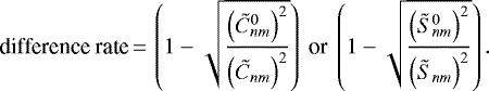$$\text{difference rate}=\left(1-\sqrt{\frac{{\left({\tilde{C}}_{nm}^0\right)}^2}{{\left({\tilde{C}}_{nm}\right)}^2}}\right)\text{or}\left(1-\sqrt{\frac{{\left({\tilde{S}}_{nm}^0\right)}^2}{{\left({\tilde{S}}_{nm}\right)}^2}}\right).$$(21)

For any tesseral or sectoral coefficients that are assumed to be nonzero, namely ${\tilde{C}}_{nm}^0,{\tilde{S}}_{nm}^0\ne 0$, an excellent recovery is shown by the difference rate being close to zero. If the POD of a simulated mission fails to reasonably reproduce the gravitational field model, it strongly indicates that the corresponding orbit configuration is incapable of detecting the gravitational signature we are interested in. As a result, the feasibility and quality of the gravity determination of a mission can be judged, with regard to the interested phenomenon (e.g., in this work, the dynamo-related tesseral or sectoral coefficients). Hereafter, following the above discussed simulation principle, we show that the five gravity-measuring arcs of the Grand Finale orbits are unlikely to have determined the static tesseral or sectoral gravitational moments that are linked to the typical deep convective distortions of the planet because the subspacecraft-point coverage of these orbits was limited.

Technically speaking, a simulated POD procedure consists of nearly all physical and technical ingredients that are encountered in a real mission, but the main gravitational field of the primary object, namely Saturn in this study, is given by a model, either Table 2 plus Table 1 or Table 3 plus Table 1. Secondary perturbative gravity from other solar or Saturnian system objects (Folkner et al. 2008) and relativistic post-Newtonian effects (Moyer 2005) are included, exactly within the coherent time interval and coordinate system of the simulation, and combined with the main gravitation, composing the overall force model that governs the motion of a spacecraft. This motion is then supposed to be tracked by radio measures, taking the observational architectures that are referred to the real mission into account. Table 4 summarizes our relevant POD setting for asimulated Cassini Grand Finale-like mission. Through this simulation, we can test whether the desired gravitational field can be recovered under the conditions that best resemble those of the Cassini Grand Finale mission.

Simulated orbit-tracking tasks were performed as if they were carried out by the antennas of three complexes (Madrid in Spain; Goldstone in the USA; and Canberra in Australia) in the NASA Deep Space Network (DSN), in addition to two deep-space antennas from ESA’s ESTRACK network, located in the southern hemisphere (Malargüe in Argentina, and New Norcia in Australia) (Iess et al. 2019). The precise station coordinates are listed in Table 5. The level of observational noise of the tracking data in the simulations is also given with reference to the Cassini Grand Finale mission (Iess et al. 2019), in which data quality is statistically equivalent in X- and Ka-band data, with a root-mean-square (RMS) Doppler noise of about 0.02 mm s⁻¹ at 30 s integration time (Durante 2017). In addition to the nominal accuracy, the observation scheduling also repeats that of the realistic mission. These configurations and tracking stations are used in all the following sections.

All the POD simulations were performed using a stable version of Wuhan University Deep space Orbit determination and Gravity recovery System (WUDOGS), an in-house developed software. It has been used in Moon (Yan et al. 2020; Liu et al. 2020), Mars (Yan et al. 2018; Yang et al. 2019), Mercury (Yan et al. 2019), and asteroid missions (Jin et al. 2020).

3.2 Simulated Cassini-like missions and resulting solutions

The first reported simulations are claimed to be Cassini-like, mainly because the predominant zonal gravitational moments of Saturn (see Table 1) are retained in the constructed models of the gravitational field. As a result, starting with an initial osculating orbit, our test spacecraft would approximately follow the Cassini Grand Finale trajectory well. Key features of the dynamics revealed in the simulations therefore represent those of the real mission. Table 6 presents the initial orbit elements for five orbital arcs, including perifocal distance, eccentricity, inclination, ascending node longitude, argument of periapsis, and mean anomaly as retrieved from the SPICE Toolkit of the Navigation and Ancillary Information Facility (NAIF; Acton 1996; Acton et al. 2018). In Fig. 2 one set of the simulated orbits is plotted to illustrate the closest approaches in ICRF equatorial coordinates at epoch J2000.0. The simulated Doppler data were acquired with the WUDOGS software. These data were then fed into a multi-arc weighted least-squares estimation filter, outputting solved gravitational harmonics coefficients and their one-sigma uncertainty up to spherical harmonics of degree 20. Reported gravitational field solutions are further truncated up to degree 12, consistent with the Cassini Grand Finale mission results. By always including sufficiently more degrees of harmonics in the estimation process, aliasing and false small correlations between the high-degree parameters due to truncation can be avoided.

The Cassini-like missions were conducted for gravitational field models with the strong-field and weak-field dynamo. The two POD gravitational field solutions were then assessed in terms of difference rate, defined by Eq. (21). According to the results presented in Fig. 3, neither the strong-field dynamo-related ${\tilde{S}}_{n2}$ coefficients nor the weak-field dynamo-related ${\tilde{S}}_{n9}$ coefficients are apparently solved correctly.

By virtue of the simulations, it becomes obvious that the five Grand Finale orbital arcs, which were dedicated to gravity determination, cannot solve the tesseral and sectoral gravitational moments of Saturn. The implication is twofold. First, for a deep convective flow of typical strength, regardless of whether it belongs to the category of strong-field or weak-field dynamo, its distortions in gravitational moments cannot be precisely detected under the orbit configuration of the Cassini Grand Finale mission. Second, on the other hand, this also means that the Cassini Grand Finale mission was not inherently able to assert a persistent existence, or absence, of nonaxisymmetric gravitational moments, even though a negative view was presented in Iess et al. (2019). As a result, in the era of the Cassini mission, it is still left unclear whether the convective dynamo of Saturn can be detected through gravitational sounding.

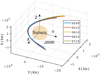Fig. 2 Selected orbit ephemerides. Tracking observables are based on five arcs, using mock Doppler observations with 30-s integrating interval time, spanning 24 h about each closest approach.

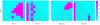Fig. 3 Difference rate for all orders and degrees of the gravitational harmonics coefficients that are involved in our POD simulations. Panels a and b: present the case marked by m0 = 2, belonging to the strong-field dynamo category, and the case marked by m0 = 9, belonging to the weak-field dynamo category, respectively. In either panel, the left part plots the different rate of ${\tilde{C}}_{nm}$ coefficients, and the right part plots the rate of ${\tilde{S}}_{nm}$. The zeroth-order ${\tilde{C}}_{0m}$ coefficients are in essence the zonal harmonics coefficients ${\tilde{J}}_n$. In the case shown in panel a, the input gravitational harmonics coefficients are all null, except for nonzero zonal coefficients of all degrees and nonzero ${\tilde{S}}_{n2}^0, n=2,3,5,7,9$. In the other case of panel b, the modeled nonzero tesseral and sectoral coefficients become ${\tilde{S}}_{n9}^0, n=9,10,11,12$. The difference rate only applies to coefficients that are assumed to be nonzero, as highlighted in all panels by boxes with dashed black edges.

4 Extensive orbit search to detect the Saturnian convective dynamo

The experience of Pioneer and Voyager missions shows that flyby orbits are not sufficient to accurately solve the nonaxisymmetric gravitational coefficients at a reasonable level. Our simulations have further demonstrated that the Cassini Grand Finale orbits were also not sensitive to the targeted nonaxisymmetric gravitational moments, even though the closest approaches of the spacecraft reached down to about 3000 km to the Saturn surface, between Saturn and its D-ring. Clearly, detecting the Saturnian convective dynamo through gravitational field measurements demands more in the orbit design of a mission. To better understand the problem and to facilitate future orbit design, more simulated missions were carried out under complex conditions. We tested not only orbits with several different combinations of perifocal distance, inclination, and eccentricity, but also the convective flow strength, which is characterized by ${\mathcal{U}}_0$. We allowed it to vary between 0.1 and 10 m s⁻¹.

4.1 Ideal near-circular orbits and feasibility of gravitational sounding

Our trials started with near-circular orbits with different inclinations and altitudes, as illustrated in Fig. 4. Near-circular and low-fly orbits theoretically provide a gravity determination with the best conditions and hence require the shortest POD tracking time. Therefore it is expected that these orbits offer a channel for investigating the minimum required efforts. Any feasible missions would thus be more expensive and challenging if a similar level of gravity determination were desired. The angles of 30°, 60°, and 89° represent low, medium, and high orbital inclinations, respectively. Three orbital elevations, 1000, 3000, and 6000 km, from the cloud top of Saturn were selected, which are all located well between Saturn and its ring system. Generally speaking, low eccentricity and low altitude are the most favorable combination for gravity determination. We claim that these orbital configurations only bear theoretical significance rather than engineering feasibility. Only through these best-fit simulationscan the minimum requirements of mission scheduling be determined, however, and these simulations can thus help estimate the practicality and difficulty of carrying out any real missions. In addition to the spatial structure of orbits, another crucial factor is the POD tracking time. A longer orbit-tracking time usually leads to better sub-spacecraft-point coverage, more abundant effective observational data, and hence better quality in gravity determination. The orbit-tracking tasks were set to last seven days, one month, or three months. Based on the inclination angle, orbit height, and tracking-time settings, in this round of mission simulations, we sampled 3 × 3 × 3 = 27 permutations of orbiting strategies in total. To all other technical features of the POD simulations applies what we discussed in Sect. 3.

The convective strength in the Saturn dynamo region was assumed to be ${\mathcal{U}}_0=1\text{m}{\text{s}}^{-1}$ in the previous section. Equation (16) shows and Sect. 2 discussed that the flow-induced gravitational moments linearly scale with ${\mathcal{U}}_0$. As a result, successful gravitational sounding will offer direct constraints of the typical speed of the dynamo flow. To account for more possibilities of flow strength, we further set ${\mathcal{U}}_0$ through 0.1 to 10 m s⁻¹, yielding 19 gravitational field models in toal. The possibility is very high that the typical flow speed in the dynamo region of Saturn is O(1) m s⁻¹, otherwise it would violate the basic MHD balance (Starchenko & Jones 2002). In other words, the speed range 0.1–10 m s⁻¹ covers possible dynamical conditions well.

The model we examined first was the strong-field dynamo case, whose flow distortion is marked by an m₀ = 2 azimuthal variation. When ${\mathcal{U}}_0=1 \text{m}{\text{s}}^{-1}$, the nonaxisymmetric gravitational moments are given in Table 2. For any other values of ${\mathcal{U}}_0$, the corresponding gravitational coefficients were simply obtained by linearly scaling the numbers in Table 2. Applying the 19 strong-field dynamo-type gravitational field models with the 27 orbiting strategies, we conducted POD simulations and display the difference rate of the targeted tesseral and sectoral coefficients between the forward gravitational field models and gravitational field solutions in Fig. 5.

The most profound conclusion to be drawn from Fig. 5 is that gravitational sounding to detect the dynamo-related signatures is possible, at least for near-circular and low-altitude orbits. Some common facts with respect to orbit configurations can also be straightforwardly inferred. A higher inclination angle is better, and a longer POD tracking time certainly improves the quality of solutions. For a particular orbiting and tracking schedule, lower degree gravitational coefficients and stronger gravitational signatures produced by faster flows are easier to be determined effectively, as expected. More precisely, a polar orbit is the most advantageous strategy. A three-month tracking time will thus safely enable a successful detection of all degrees of the targeted gravitational coefficients, even for those arising from the weakest flow of ${\mathcal{U}}_0=0.1 \text{m}{\text{s}}^{-1}$. If the tracking time needs to be dramatically shortened to several days, however, it is still likely to partly tell with confidence the lower-degree (n < 6) gravitational moments. However, if a moderate inclination angle has to be in place, then a three-month tracking time together with an ultra-low altitude orbit, 1000 km for example, may work.

Next, we examined the weak-field dynamo scenario, in which the convective dynamo causes an azimuthally m₀ = 9 distortion (cf. Table 3) of the primary gravitational field. All orbiting and POD settings remained unchanged. Similarly, the difference rate of the targeted tesseral and sectoral coefficients of about m = 9 is collectively plotted in the chart in Fig. 6. More difficulties in detecting higher order gravitational coefficients are expected because they are generally much weaker. Compared to the previously discussed situation of the m₀ = 2 strong-field dynamo case, additional challenges are demonstrated in Fig. 6. A longer orbit-tracking time and lower orbit height are requireed, even for the most superior polar orbit strategy. In particular, a higher azimuthal wave number of the gravitational signature requires higher spatial resolution, which is naturally obtained by decreasing the orbit height.

Although the difference rate values have reflected the accuracy of gravitation solutions, in order to convincingly determine the detectability of physical model parameters, it is also necessary and crucial to examine the formal uncertainty. Three relevant RMS quantities are introduced for this purpose, $$\begin{array}{lll}{\sigma }_n\hfill & =\hfill & \sqrt{\frac{{\Sigma }_{m=0}^n({\tilde{C}}_{nm}^2+{\tilde{S}}_{nm}^2)}{2n+1}},\hfill \\ {\delta }_n\hfill & =\hfill & \sqrt{\frac{{\Sigma }_{m=0}^n(\delta {\tilde{C}}_{nm}^2+\delta {\tilde{S}}_{nm}^2)}{2n+1}},\hfill \\ {\Delta }_n\hfill & =\hfill & \sqrt{\frac{{\Sigma }_{m=0}^n(\Delta {\tilde{C}}_{nm}^2+\Delta {\tilde{S}}_{nm}^2)}{2n+1}}.\hfill \end{array}$$

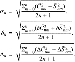
The first, σ_n (n = 2, 3, …) depicts the degree-wise spectrum of a particular set of gravitational moments ${\tilde{C}}_{nm},{\tilde{S}}_{nm}$. The second, δ_n (n = 2, 3, …), the spectrum of the formal error, is computed based on the one-sigma uncertainty of a solution of gravitational moments $\delta {\tilde{C}}_{nm},\delta {\tilde{S}}_{nm}$. They directly show the intrinsic precision of the solution. The third, Δ_n (n = 2, 3, …) is calculated from the coefficient-wise differences $\Delta {\tilde{C}}_{nm},\Delta {\tilde{S}}_{nm}$ between any two different sets of gravitational moments. If $\Delta {\tilde{C}}_{nm}$ and $\Delta {\tilde{S}}_{nm}$ are evaluated between the solution (${\tilde{C}}_{nm}$, ${\tilde{S}}_{nm}$) and the model (${\tilde{C}}_{nm}^0$, ${\tilde{S}}_{nm}^0$), then the Δ_n spectrum tells the accuracy of the solution, delivering a conceptually similar message as the difference rate.

By virtue of these definitions, the successful mission schedules, which are highlighted by the red line boxes in Figs. 5 and 6, are verified. Several power spectra of σ_n, δ_n, and Δ_n are plotted in Fig. 7 with regard to degree n. For our simulations, all degree-wise formal uncertainties of the gravity solutions are well lower than spectral intensity of the coefficients. Figures 5–7 together show that the designated orbits indeed deliver the desired gravitational signatures.

We emphasize again that in this subsection, all conducted missions have assumed near-circular orbits that reside within the rings of Saturn. In the near future, it appears to be highly unlikely that such orbits are implemented because of tremendous engineering difficulties. Nevertheless, these studies are worthy for two reasons. First, it is now proven that gravitational sounding is essentially able to detect the Saturnian convective dynamo, which inspires further explorations into more practical missions. Second, the ideal missions we simulated offer insight into the complex factors that affect the effectiveness of gravity determination, which supports and guides future mission design.

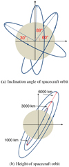Fig. 4 Best-fit near-circular orbits for conducting gravitational sounding of the Saturnian convective dynamo. We show three inclination angles, 30°, 60°, and 89°, and three orbit heights, 1000, 3000, and 6000 km from the Saturn cloud top.

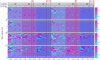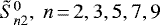
Fig. 5 Difference rate of the targeted tesseral and sectoral coefficient solutions in the case of m0 = 2. The targeted coefficients are ${\tilde{S}}_{22}$, ${\tilde{S}}_{32}$, ${\tilde{S}}_{42}$, ${\tilde{S}}_{52}$, ${\tilde{S}}_{62}$, ${\tilde{S}}_{72}$, ${\tilde{S}}_{82}$, and ${\tilde{S}}_{92}$. For each coefficient, the light green, light red, and light gray columns indicate three different inclination angles of 30°, 60°, and 89°. Each column has three subcolumns, arranged according to the orbit-tracking time of seven days, one month, and three months. Each subcolumn is further separated into another three subcolumns of 1, 3, and 6 km elevation of the orbit above the Saturn cloud-top surface. The row dimension labels different forward gravitational field models resulting from different convective flow speeds ${\mathcal{U}}_0$ that are sampled into 19 cases of 0.1, 0.2, 0.3, 0.4, 0.5, 0.6, 0.7, 0.8, 0.9, 1, 2, 3, 4, 5, 6, 7, 8, 9, and 10 m s−1. The red lineboxes drawn on top of the chart figure, labeled a, b, c, and d, denote the candidate mission schedules that successfully detect the strong-field dynamo.

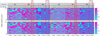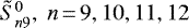
Fig. 6 Difference rate of the targeted tesseral and sectoral coefficient solutions in the case of the m0 = 9 weak-field dynamo. The targeted coefficients are ${\tilde{S}}_{99}$, ${\tilde{S}}_{10,9}$, ${\tilde{S}}_{11,9}$, and ${\tilde{S}}_{12,9}$. The red lineboxes drawn on top of the chart figure, with legends e, f and g, denote the candidate mission schedules that successfully detect the weak-field dynamo. Explanations of the layout of this chart are the same as in the caption of Fig. 5.

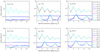Fig. 7 Degree-wise spectra of RMS quantities σn, δn, and Δn for several specified cases. Top panels: plot the strong-field dynamo category (m0 = 2), and bottom three panels: weak-field dynamo category (m0 = 9). The panel columns are permuted from left to right in ascending order of the convective strength ${\mathcal{U}}_0$. In the curve legends, each subscript labels a respective mission simulation schedule. 6013 denotes the 60° orbital inclination angle, 1000 km altitude, and three-month tracking time. 8913 denotes the 89° orbital inclination angle, 1000 km altitude, and three-month tracking time. 8933 also denotes the 89° orbital inclination angle, 3000 km altitude, and three-month tracking time. The label “FM” is the abbreviation for “forward model”, which means that σn is computed from ${\tilde{C}}_{nm}^0$ and ${\tilde{S}}_{nm}^0$. Here Δn is always calculated between mission solutions and the given gravitational field models, as given in Tables 1–3.

4.2 Orbits of moderate eccentricity and potential application in gravitational sounding

Based on the experience and confidence we gained, we proceeded with more mission simulations, with a more balanced consideration between desire and practicality. In real missions to gaseous giant planets, such as the Juno or Cassini missions, orbits with higher eccentricity are preferred for several remarkable reasons. Less fuel is required to brake and insert the spacecraft into a high-eccentricity orbit. More importantly, a highly elliptic trajectory keeps the spacecraft away from hazardous planetary radiation belts. However, the disadvantage is also obvious. In terms of observing the planet, only the arcs of the orbits that are near the periapsides are effective. Most of mission time is less useful when the spacecraft remains distant from the planet. In this subsection, we propose a moderately eccentric polar orbit around Saturn and verify its power of detecting the Saturnian convective dynamo.

To design a proper orbit, we can learn from the previous extensive examples. In Fig. 8 we plot subspacecraft points for several cases. We present two failed cases (panels a and b) together with two successful cases (panels c and d). The comparison between them provides an inspiring vision of the crucial factor that affects the quality of gravity determinations. The coverage of subspacecraft points during the POD tracking period clearly plays an important role. When the coverage is poor or limited, which can be attributed to low orbit inclination or short tracking time (short arc length) or both, the nonaxisymmetric gravitational moments cannot be solved coherently and correctly.

Our extensive simulations indicated that a good coverage of the subspacecraft points is crucial. Meanwhile, to apply this to a designed orbit in a Saturn mission, it is also necessary to consider engineering practicality as well as possible. We finally propose the orbit that is shown by the solid black line in Fig. 9. The near-polar orientation of the orbit ensures that both polar caps are well covered, unlike the unfavorable situation of panel c in Fig. 8. The choice of the orbital eccentricity is a compromise of two opposite demands. For the sake of determining the gravity, lower eccentricity will certainly be preferred because it is in favor of a coherent coverage of the subspacecraft points, which enhances the sensitivity of POD to the nonaxisymmetric gravitational field. On the other hand, engineers would eagerly request that the spacecraft is kept from energetic particles in the planetary radiation belts. In our proposal, the orbital eccentricity is selected to be 0.5, together with a perifocal height of about 6000 km above the Saturn cloud top. This orbit configuration maintains a 2 × 10⁵ km apoapsis distance, which is just enough for the spacecraft to marginally avoid the densest radiation belts of Saturn and reach 3.5R_S at most (Andre et al. 2008).

Our ultimate objective is to detect dynamo-related nonaxisymmetric gravitational moments. We carried out POD simulations for the designated polar orbits of moderate eccentricity 0.5. The solutions for the case of the strong-field dynamo are tabulated in Table 7, where the targeted nonaxisymmetric gravitational moments would be fairly well determined to all degrees if a five-month tracking time were achieved. However, a similar result is notreasonably obtained in the regime of the weak-field dynamo, where the gravitational signature is marked by a smaller azimuthal scale. We expect that a much longer Doppler orbit tracking would be required, during which spacecraft manoeuvres may be inevitable for the purpose of orbit maintenance. With the available knowledge, it has fortunately been more than enough to assess the features of the dynamo process. If a lower order (m = 2, 3, …) spectrum is outstanding in the gravitational field, it is indicative of a large Elsasser number in the dynamo region, namely, the strong-field dynamo. The gravitational sounding can further constrain the typical flow strength of the dynamo. Conversely, if no predominant lower order gravitational moments are detected, the null result can probably be interpreted as meaning that the dynamo belongs to the weak-field category.

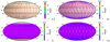Fig. 8 Subspacecraft-point coverage of typical missions. Panel a: actual subspacecraft points of the five Cassini Grand Finale closest approaches. The global coverage is very limited, and the orbit height from the Saturn surface inherently differs much at different latitudes because of the high orbital eccentricity. Panel b: fairly sparse subspacecraft-point coverage is plotted for the simulated missions of near-circular polar orbits and seven-day POD tracking time. Panels c and d: demonstrate two circumstances under which the targeted tesseral and sectoral gravitational coefficients can be solved from POD simulations. Panel c: plotted mission adopts a 1000 km high, 60° medium-inclination orbit, and the tracking time is three months. Panel d: simulated missions tracked for three months with polar orbits.

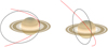Fig. 9 Proposed moderately eccentric polar orbit to gravitationally detect the Saturnian convective dynamo. The two panels plot the same thing from different viewing angles. The red line illustrates one closest approach of the Cassini Grand Finale orbits, with an inclination of about 57° and an eccentricity of almost 0.9. The black line draws an instantly osculating orbit of our proposed moderate-eccentricity orbits. The orbit takes a near-polar orientation, with 89° inclination. The minimum height from the Saturn cloud top at its periapsis is 6000 km, well inside of the ring system of Saturn. The orbital eccentricity is 0.5, which gives a 2 × 105 km apoapsis. The two apsides lie in the equatorial plane of Saturn.

4.3 Additional considerations of data interpretation

In our simulations, the spacecraft flies in modeled gravitational fields, of which the nonaxisymmetric components are purely related to dynamo flows. However, in real life, this is more complicated. Multiple intrinsic sources of a nonaxisymmetric gravitational field exist, such as tides, free oscillations, and even major atmospheric streams. A spacecraft always measures the total gravitational field. Data will not automatically split into components of different origins. As a result, based on the POD simulations, we only claim that gravitational sounding is a viable approach insofar as its sensitivity is high enough to detect dynamo-related gravitational signatures. For any practical data interpretation, however, the dynamo-related part of the overall gravitational field can only be retrieved when a comprehensive model of the nonaxisymmetric gravitational field is established.

Although it is beyond the scope of this paper to interpret any real data, it is helpful to consider this question briefly. First, tides and free oscillations have fast temporal variations (of hours, days, or months), but dynamo-related signatures are secular (changing on a magnetic diffusion timescale). This obvious discrepancy might be useful to separate gravitational components in the frequency domain. Second, atmospheric vortices and some seasonal (in the Saturn concept of season) atmosphericmotions only distort a relatively localized part in the outer atmosphere. They might not cause gravitational anomalies at a global scale. In a future mission, gravitational sounding of the Saturnian convective dynamo might be feasible.

5 Conclusions and perspectives

The planetary dynamo of gaseous giant planets is one of the most intractable problems to explore because of its complexity. Dynamo equations combine momentum, heat, and magnetic induction equations; they represent the advection-diffusion dynamics of fluid momentum, thermal energy, and the magnetic field. The three diffusion coefficients kinematic viscosity ν, thermal diffusivity κ, and magnetic diffusivity η = 1∕(μ₀σ), mark three unique timescales of the evolution of the dynamical system. The three important coefficients when taken together with the planetary rotation rate Ω₀ control the dynamo process. In fluid dynamics research, following the law of similarity, a few dimensionless parameters combine physical coefficients and determine the nature of dynamics. These parameters mainly include the Ekman number, $E_k=\frac{\nu }{{\Omega }_0{R}_S{}^2}$, which measures the relative importance between viscous force and Coriolis force, the Prandtl number, Pr$=\frac{\nu }{\kappa }$, which compares the viscous timescale with the thermal diffusion timescale, and the magnetic Prandtl number, $Pm=\frac{\nu }{\eta }$, which compares the viscous timescale with the magnetic diffusion timescale. In the astrophysical context, dynamo processes can demonstrate varieties of types, depending on the location of their internal physical states in the parameter space (Christensen et al. 2008). Theoretically, for a particular celestial object, for example, a planet, if we can determine these parameters, the dynamo process can be studied; however, we understand little about this for any planet. More critically, fast rotation and a typically O(10³−10⁴) km length scale in the case of gaseous planets results in an extremely small Ekman number, which is one of the key factors preventing reliable numerical simulations (Zhang & Liao 2017).Thus, forward dynamo calculations are made with asymptotically small Ekman numbers that lie within the capacity of the latest high-performance computing facilities. This has already placed our numerical dynamo model in a very unrealistic parameter space regime. Moreover, for gaseous planets such as Jupiter and Saturn, we do not even know the precise location of their operating dynamos, although qualitatively, it can be inferred that this must take place in the metallic hydrogen region. These intrinsic and appended difficulties have made forward studies of gaseous planets dynamos challenging.

After observing the tremendous difficulties and uncertainties in forward dynamo calculations, we have presented a novel idea of using gravitational sounding to inversely diagnose the planetary dynamo in gaseous planets. The connection between dynamo and gravity is the density anomaly caused by the convective flow. We mathematically computed the density anomaly and hence gravitational signature resulting from a dynamo convective flow that is parameterized with a typical flow speed ${\mathcal{U}}_0$, azimuthal wave number m₀, and geometric domain of the dynamo region. With this method, two typical categories of dynamo processes were considered for Saturn. One is the so-called weak-field dynamo, whose convective motion structure, although substantially affected by the magnetic field, is still more predominantly controlled by rotational effects; the other category is called strong-field dynamo, in which the Lorentz force dominates the fluid dynamics. For a weak-field dynamo, the convective pattern usually admits a small azimuthal scale because of the condition Ek ≪ 1 and Pr/Ek ≫ 1 (Zhang & Liao 2004). In the other category, if the dynamo is of strong-field type, its convective motion is usually marked by a large-scale azimuthal structure. An outstanding fact therefore is that the two types of dynamo can be distinguished by measuring their associated gravitational anomalies.

The Juno and Cassini Grand Finale missions have both conducted unprecedentedly high accurate gravitational field measurements for Jupiter and Saturn, respectively. Especially, Iess et al. (2019) reported unexplained nonaxisymmetric gravitational coefficients determined from a POD of the Cassini Grand Finale mission. We therefore applied the gravitational sounding method as discussed to determine whether this feature can be attributed to the Saturnian convective dynamo. Our POD simulations have demonstrated a negative conclusion. In essence, the Cassini Grand Finale orbits cannot reliably solve the gravitational signature that is related to the Saturnian convective dynamo, which means that the source of the unexplainedgravity remains a puzzle even after the mission. We also completed other extensive simulations of spacecraft orbits with various eccentricities, heights, inclinations, and lengths of tracking time. Our simulations support the feasibility of detecting the Saturnian convective dynamo through the gravitational sounding method. The subspacecraft-point coverage plays the most fundamental role in gravity determination. This is to facilitate future Saturn missions if the diagnostic of a Saturnian convective dynamo were to become one of the scientific objectives.

Acknowledgements

D.K. is supported by the B-type Strategic Priority Program of the Chinese Academy of Sciences (Grant No. XDB41000000); by the Pre-research Project on Civil Aerospace Technologies funded by China National Space Administration (Grant No. D020303 and No. D020308); by the Macau Science and Technology Development Fund (Grant No. 0001/2019/A1 and No. 0005/2019/A1); and by the Hong Kong-Macau-Taiwan Cooperation Funding of Shanghai Committee of Science and Technology (Grant No. 19590761300). J.Y. is supported by National Scientific Foundation of China (Grant No. U1831132 and 41374024); by Innovation Group of Natural Fund of Hubei province (Grant No. 2018CFA087). The computation made use of the high-performance computing resources in the Core Facility for Advanced Research Computing at Shanghai Astronomical Observatory, Chinese Academy of Sciences.

References

All Tables

All Figures

Fig. 1 Sketch of a possible convective flow inside the metallic hydrogen-helium region of Saturn. The cylindrical pattern of fluid motions (∂u∕∂z = 0) reflects the fast-rotation effect (Zhang & Liao 2017), and the azimuthal number of columns indicates the typeof dynamo action (Zhang & Jones 1996). The flow has an azimuthal wave number 2, whichillustrates a possible convection of the strong-field dynamo (e.g., see Elsasser number Λ = 5.1 in Fig. 6 of Zhang 1995).

In the text

	Fig. 2 Selected orbit ephemerides. Tracking observables are based on five arcs, using mock Doppler observations with 30-s integrating interval time, spanning 24 h about each closest approach.
In the text

Fig. 3 Difference rate for all orders and degrees of the gravitational harmonics coefficients that are involved in our POD simulations. Panels a and b: present the case marked by m0 = 2, belonging to the strong-field dynamo category, and the case marked by m0 = 9, belonging to the weak-field dynamo category, respectively. In either panel, the left part plots the different rate of ${\tilde{C}}_{nm}$ coefficients, and the right part plots the rate of ${\tilde{S}}_{nm}$. The zeroth-order ${\tilde{C}}_{0m}$ coefficients are in essence the zonal harmonics coefficients ${\tilde{J}}_n$. In the case shown in panel a, the input gravitational harmonics coefficients are all null, except for nonzero zonal coefficients of all degrees and nonzero ${\tilde{S}}_{n2}^0, n=2,3,5,7,9$. In the other case of panel b, the modeled nonzero tesseral and sectoral coefficients become ${\tilde{S}}_{n9}^0, n=9,10,11,12$. The difference rate only applies to coefficients that are assumed to be nonzero, as highlighted in all panels by boxes with dashed black edges.

In the text

	Fig. 4 Best-fit near-circular orbits for conducting gravitational sounding of the Saturnian convective dynamo. We show three inclination angles, 30°, 60°, and 89°, and three orbit heights, 1000, 3000, and 6000 km from the Saturn cloud top.
In the text

Fig. 5 Difference rate of the targeted tesseral and sectoral coefficient solutions in the case of m0 = 2. The targeted coefficients are ${\tilde{S}}_{22}$, ${\tilde{S}}_{32}$, ${\tilde{S}}_{42}$, ${\tilde{S}}_{52}$, ${\tilde{S}}_{62}$, ${\tilde{S}}_{72}$, ${\tilde{S}}_{82}$, and ${\tilde{S}}_{92}$. For each coefficient, the light green, light red, and light gray columns indicate three different inclination angles of 30°, 60°, and 89°. Each column has three subcolumns, arranged according to the orbit-tracking time of seven days, one month, and three months. Each subcolumn is further separated into another three subcolumns of 1, 3, and 6 km elevation of the orbit above the Saturn cloud-top surface. The row dimension labels different forward gravitational field models resulting from different convective flow speeds ${\mathcal{U}}_0$ that are sampled into 19 cases of 0.1, 0.2, 0.3, 0.4, 0.5, 0.6, 0.7, 0.8, 0.9, 1, 2, 3, 4, 5, 6, 7, 8, 9, and 10 m s−1. The red lineboxes drawn on top of the chart figure, labeled a, b, c, and d, denote the candidate mission schedules that successfully detect the strong-field dynamo.

In the text

Fig. 6 Difference rate of the targeted tesseral and sectoral coefficient solutions in the case of the m0 = 9 weak-field dynamo. The targeted coefficients are ${\tilde{S}}_{99}$, ${\tilde{S}}_{10,9}$, ${\tilde{S}}_{11,9}$, and ${\tilde{S}}_{12,9}$. The red lineboxes drawn on top of the chart figure, with legends e, f and g, denote the candidate mission schedules that successfully detect the weak-field dynamo. Explanations of the layout of this chart are the same as in the caption of Fig. 5.

In the text

Fig. 7 Degree-wise spectra of RMS quantities σn, δn, and Δn for several specified cases. Top panels: plot the strong-field dynamo category (m0 = 2), and bottom three panels: weak-field dynamo category (m0 = 9). The panel columns are permuted from left to right in ascending order of the convective strength ${\mathcal{U}}_0$. In the curve legends, each subscript labels a respective mission simulation schedule. 6013 denotes the 60° orbital inclination angle, 1000 km altitude, and three-month tracking time. 8913 denotes the 89° orbital inclination angle, 1000 km altitude, and three-month tracking time. 8933 also denotes the 89° orbital inclination angle, 3000 km altitude, and three-month tracking time. The label “FM” is the abbreviation for “forward model”, which means that σn is computed from ${\tilde{C}}_{nm}^0$ and ${\tilde{S}}_{nm}^0$. Here Δn is always calculated between mission solutions and the given gravitational field models, as given in Tables 1–3.

In the text

Fig. 8 Subspacecraft-point coverage of typical missions. Panel a: actual subspacecraft points of the five Cassini Grand Finale closest approaches. The global coverage is very limited, and the orbit height from the Saturn surface inherently differs much at different latitudes because of the high orbital eccentricity. Panel b: fairly sparse subspacecraft-point coverage is plotted for the simulated missions of near-circular polar orbits and seven-day POD tracking time. Panels c and d: demonstrate two circumstances under which the targeted tesseral and sectoral gravitational coefficients can be solved from POD simulations. Panel c: plotted mission adopts a 1000 km high, 60° medium-inclination orbit, and the tracking time is three months. Panel d: simulated missions tracked for three months with polar orbits.

In the text

Fig. 9 Proposed moderately eccentric polar orbit to gravitationally detect the Saturnian convective dynamo. The two panels plot the same thing from different viewing angles. The red line illustrates one closest approach of the Cassini Grand Finale orbits, with an inclination of about 57° and an eccentricity of almost 0.9. The black line draws an instantly osculating orbit of our proposed moderate-eccentricity orbits. The orbit takes a near-polar orientation, with 89° inclination. The minimum height from the Saturn cloud top at its periapsis is 6000 km, well inside of the ring system of Saturn. The orbital eccentricity is 0.5, which gives a 2 × 105 km apoapsis. The two apsides lie in the equatorial plane of Saturn.

In the text

References

- Acton, Jr. C. H. 1996, Planet. Space Sci., 44, 65 [NASA ADS] [CrossRef] [Google Scholar]
- Acton, Jr. C. H., Bachman, N., Semenov, B., & Wright, E. 2018, Planet. Space Sci., 150, 9 [NASA ADS] [CrossRef] [Google Scholar]
- Anderson, J. D., & Schubert, G. 2007, Science, 317, 1384 [NASA ADS] [CrossRef] [Google Scholar]
- Andre, N., Blanc, M., Maurice, S., et al. 2008, Rev. Geophys., 46, RG4008 [CrossRef] [Google Scholar]
- Archinal, B. A., Acton, C. H., A’Hearn, M. F., et al. 2018, Celest. Mech. Dyn. Astr., 130, 22 [NASA ADS] [CrossRef] [Google Scholar]
- Buffett, B. A. 2000, Science, 288, 2007 [NASA ADS] [CrossRef] [Google Scholar]
- Campbell, J., & Anderson, J. 1989, AJ, 97, 1485 [NASA ADS] [CrossRef] [Google Scholar]
- Chandrasekhar, S. 1962, Hydrodynamic and Hydromagnetic Stability (Oxford: Clarendon Press) [Google Scholar]
- Christensen, U. R., Holzwarth, V., & Reiners, A. 2008, Nature, 457, 167 [Google Scholar]
- Connerney, J. E. P., Kotsiaros, S., Oliversen, R. J., et al. 2018, Geophys. Res. Lett., 45, 2590 [NASA ADS] [CrossRef] [Google Scholar]
- Davis, J. L., Herring, T. A., Shapiro, I. I., Rogers, A. E. E., & Elgered, G. 1985, Radio Sci., 20, 1593 [NASA ADS] [CrossRef] [Google Scholar]
- Desch, M. D., & Kaiser, M. L. 1981, Geophys. Res. Lett., 8, 253 [NASA ADS] [CrossRef] [Google Scholar]
- Dougherty, M. K., Cao, H., Khurana, K. K., et al. 2018, Science, 362, 46 [CrossRef] [Google Scholar]
- Duarte, L. D. V., Gastine, T., & Wicht, J. 2013, Phys. the Earth Planet. Inter., 222, 22 [NASA ADS] [CrossRef] [Google Scholar]
- Durante, D. 2017, The gravity fields of Jupiter and Saturn as determined by Juno and Cassini (Sapienza Universita de Roma) [Google Scholar]
- Edgington, S. G., & Spilker, L. J. 2016, Nat. Geosci., 9, 472 [CrossRef] [Google Scholar]
- Folkner, W. M., Williams, J. G., & Boggs, D. H. 2008, JPL IOM 343R-08-003 [Google Scholar]
- Glatzmaier, G. A. 2002, Ann. Rev. Earth Planet. Sci., 30, 237 [CrossRef] [Google Scholar]
- Glatzmaier, G. A. 2018, Proc. National Academy of Sciences, 115, 6896 [CrossRef] [Google Scholar]
- Guillot, T. 2005, Ann. Rev. Earth Planet. Sci., 33, 493 [NASA ADS] [CrossRef] [MathSciNet] [PubMed] [Google Scholar]
- Helled, R., Schubert, G., & Anderson, J. D. 2009, Icarus, 199, 368 [NASA ADS] [CrossRef] [Google Scholar]
- Helled, R., Galanti, E., & Kaspi, Y. 2015, Nature, 520, 202 [NASA ADS] [CrossRef] [Google Scholar]
- Hopfield, H. S. 1963, J. Geophys. Res., 68, 5157 [NASA ADS] [CrossRef] [Google Scholar]
- Hubbard, W. B. 1999, Icarus, 137, 357 [NASA ADS] [CrossRef] [Google Scholar]
- Iess, L., Militzer, B., Kaspi, Y., et al. 2019, Science, 364, eaat2965 [CrossRef] [Google Scholar]
- Jacobson, R., Antreasian, P., Bordi, J., et al. 2006, AJ, 132, 2520 [NASA ADS] [CrossRef] [Google Scholar]
- Jin, W., Li, F., Yan, J., et al. 2020, MNRAS, 493, 4012 [CrossRef] [Google Scholar]
- Jones, C. A. 2014, Icarus, 241, 148 [NASA ADS] [CrossRef] [Google Scholar]
- Kaspi, Y., Galanti, E., & Hubbard, W. B. 2018, Nature, 555, 223 [NASA ADS] [CrossRef] [PubMed] [Google Scholar]
- Kong, D., Liao, X., Zhang, K., & Schubert, G. 2014, ApJ, 791, L24 [CrossRef] [Google Scholar]
- Kong, D., Zhang, K., & Schubert, G. 2016, Sci. Rep., 6, 23497 [CrossRef] [Google Scholar]
- Kong, D., Zhang, K., Schubert, G., & Anderson, J. D. 2018a, Proc. National Academy of Sciences, 155, 8499 [CrossRef] [Google Scholar]
- Kong, D., Zhang, K., Schubert, G., & Anderson, J. D. 2018b, Res. Astron. Astrophys., 18, 38 [CrossRef] [Google Scholar]
- Kong, D., Zhang, K., & Schubert, G. 2019, MNRAS, 488, 5633 [CrossRef] [Google Scholar]
- Kulowski, L., Cao, H., & Bloxham, J. 2020, J. Geophys. Res. Planets, 125, e2019JE006165 [CrossRef] [Google Scholar]
- Lagrange, R., Meunier, P., Nadal, F., & Eloy, C. 2011, J. Fluid Mech., 666, 104 [CrossRef] [Google Scholar]
- Lister, J. R., & Buffett, B. A. 1995, Phys. Earth Planet. Inter., 91, 17 [CrossRef] [Google Scholar]
- Liu, S., Yan, J., He, Q., et al. 2020, Adv. Space Res., 66, 1485 [CrossRef] [Google Scholar]
- Mandea, M., Panet, I., Lesur, V., et al. 2012, Proc. National Academy of Sciences, 109, 19129 [CrossRef] [Google Scholar]
- Militzer, B., Soubiran, F., Wahl, S. M., & Hubbard, W. B. 2016, J. Geophys. Res. Planets, 121, 1552 [NASA ADS] [CrossRef] [Google Scholar]
- Moore, K. M., Yadav, R. K., Kulowski, L., et al. 2018, Nature, 561, 76 [NASA ADS] [CrossRef] [Google Scholar]
- Moore, K. M., Cao, H., Bloxham, J., et al. 2019, Nat. Astron., 3, 730 [NASA ADS] [CrossRef] [Google Scholar]
- Morales, M. A., Schwegler, E., Ceperley, D., et al. 2009, Proc. National Academy of Sciences, 106, 1324 [NASA ADS] [CrossRef] [Google Scholar]
- Moyer, T. D. 1981, Celest. Mech., 23, 57 [CrossRef] [Google Scholar]
- Moyer, T. D. 2005, Formulation for Observed and Computed Values of Deep Space Network Data Types for Navigation, (New York: John Wiley & Sons), 3 [Google Scholar]
- Ni, D. 2020, A&A, 639, A10 [CrossRef] [EDP Sciences] [Google Scholar]
- Nicholson, P. D., & Porco, C. C. 1988, J. Geophys. Res. Solid Earth, 93, 10209 [CrossRef] [Google Scholar]
- Null, G., Lau, E., Biller, E., & Anderson, J. 1981, AJ, 86, 456 [CrossRef] [Google Scholar]
- Ogden, D. E., Glatzmaier, G. A., & Coe, R. S. 2006, Geophys. Astrophys. Fluid Dyn., 100, 107 [CrossRef] [Google Scholar]
- Otsubo, T., Matsuo, K., Aoyama, Y., et al. 2016, Earth, Planets Space, 68, 65 [CrossRef] [Google Scholar]
- Petit, G., & Luzum, B. 2010, IERS Conventions 2010 (IERS Tech. Note, 36, Bundesamts für Kartogr. und Geod., Frankfurt, Germany) [Google Scholar]
- Pozzo, M., Davies, C., Gubbins, D., & Alfe, D. 2012, Nature, 485, 355 [CrossRef] [Google Scholar]
- Stanley, S., & Glatzmaier, G. A. 2009, Space Sci. Rev., 152, 617 [NASA ADS] [CrossRef] [Google Scholar]
- Starchenko, S. V., & Jones, C. A. 2002, Icarus, 157, 426 [NASA ADS] [CrossRef] [Google Scholar]
- Stefani, F., Albrecht, T., Gerbeth, G., et al. 2014, 9th PAMIR International Conference, Fundamental and Applied MHD [Google Scholar]
- Stevenson, D. J. 1982, Ann. Rev. Earth Planet. Sci., 10, 257 [NASA ADS] [CrossRef] [Google Scholar]
- Vogt, F. P. A., Dopita, M. A., Kewley, L. J., et al. 2018, Saturn Fact Sheet, https://nssdc.gsfc.nasa.gov/planetary/factsheet/saturnfact.html [Google Scholar]
- Wood, W. W. 1966, Proc. R. Soc. Lond. A, 293, 181 [CrossRef] [Google Scholar]
- Yan, J., Yang, X., Ye, M., et al. 2018, MNRAS, 481, 4361 [NASA ADS] [CrossRef] [Google Scholar]
- Yan, J., Liu, S., Yang, X., et al. 2019, Astrophys. Space Sci., 364, 1 [CrossRef] [Google Scholar]
- Yan, J., Liu, S., Xiao, C., et al. 2020, A&A, 636, A45 [CrossRef] [EDP Sciences] [Google Scholar]
- Yang, X., Yan, J., Andert, T., et al. 2019, MNRAS, 490, 2007 [NASA ADS] [CrossRef] [Google Scholar]
- Zhan, X., Schubert, G., & Zhang, K. 2012, Icarus, 218, 345 [CrossRef] [Google Scholar]
- Zhang, K. 1995, Proc. R. Soc. Lond. A., 448, 245 [CrossRef] [Google Scholar]
- Zhang, K., & Jones, C. A. 1994, Geophys. Res. Lett., 21, 1939 [CrossRef] [Google Scholar]
- Zhang, K., & Jones, C. A. 1996, Proc. R. Soc. A, 452, 981 [CrossRef] [Google Scholar]
- Zhang, K., & Liao, X. 2004, J. Fluid Mech., 518, 319 [CrossRef] [Google Scholar]
- Zhang, K., & Liao, X. 2017, Theory and Modeling of Rotating Fluids: Convection, Inertial Waves and Precession (Cambridge: Cambridge University Press) [CrossRef] [Google Scholar]
- Zhang, K., & Schubert, G. 2000, Ann. Rev. Fluid Mech., 32, 311 [CrossRef] [Google Scholar]
All Tables
Strong-field dynamo related gravitational field coefficients computed by modeling the flow with m0 = 2.
Weak-field dynamo related gravitational field coefficients computed by modeling the flow with m0 = 9.
Configurations of the simulated missions along with the adopted orbit-tracking setup.
Gravitational field solutions for the strong-field dynamo case, obtained with the simulated missions adopting polar orbits of moderate eccentricity 0.5.