| Issue |
A&A
Volume 645, January 2021
|
|
|---|---|---|
| Article Number | A100 | |
| Number of page(s) | 13 | |
| Section | Catalogs and data | |
| DOI | https://doi.org/10.1051/0004-6361/202038827 | |
| Published online | 20 January 2021 | |
SPECULOOS: Ultracool dwarf transit survey
Target list and strategy⋆
1
Astrobiology Research Unit, University of Liège, Allée du 6 Août, 19, 4000 Liège, Sart-Tilman, Belgium
e-mail: This email address is being protected from spambots. You need JavaScript enabled to view it.
2
Cavendish Laboratory, JJ Thomson Avenue, Cambridge CB3 0HE, UK
3
Space Sciences, Technologies and Astrophysics Research (STAR) Institute, Université de Liège, Allée du 6 Août 19C, 4000 Liège, Belgium
4
Department of Earth, Atmospheric and Planetary Sciences, MIT, 77 Massachusetts Avenue, Cambridge, MA 02139, USA
5
, Chemin des Maillettes 51, Versoix 1290, Switzerland
6
University of Bern, Center for Space and Habitability, Gesellschaftsstrasse 6, 3012 Bern, Switzerland
7
School of Physics & Astronomy, University of Birmingham, Edgbaston, Birmingham B15 2TT, UK
8
University of California San Diego, 9500 Gilman Drive, La Jolla, CA 92093, USA
9
Department of Physics, University of Warwick, Coventry CV4 7AL, UK
Received:
2
July
2020
Accepted:
27
October
2020
Abstract
Context. One of the most promising avenues for the detailed study of temperate Earth-sized exoplanets is the detection of such planets in transit in front of stars that are small and near enough to make it possible to carry out a thorough atmospheric characterisation with next-generation telescopes, such as the James Webb Space telescope (JWST) or Extremely Large Telescope (ELT). In this context, the TRAPPIST-1 planets form a unique benchmark system that has garnered the interest of a large scientific community.
Aims. The SPECULOOS survey is an exoplanet transit survey targeting a volume-limited (40 pc) sample of ultracool dwarf stars (of spectral type M7 and later) that is based on a network of robotic 1 m telescopes especially designed for this survey. The strategy for brighter and earlier targets leverages on the synergy with the ongoing TESS space-based exoplanet transit survey.
Methods. We define the SPECULOOS target list as the sum of three non-overlapping sub-programmes incorporating the latest type objects (Teff ≲ 3000 K). Programme 1 features 365 dwarfs that are small and near enough to make it possible to detail atmospheric characterisation of an ‘Earth-like’ planet with the upcoming JWST. Programme 2 features 171 dwarfs of M5-type and later for which a significant detection of a planet similar to TRAPPIST-1b should be within reach of TESS. Programme 3 features 1121 dwarfs that are later than M6-type. These programmes form the basis of our statistical census of short-period planets around ultracool dwarf stars.
Results. Our compound target list includes 1657 photometrically classified late-type dwarfs, with 260 of these targets classified, for the first time, as possible nearby ultracool dwarf stars. Our general observational strategy was to monitor each target between 100 and 200 h with our telescope network, making efficient use of the synergy with TESS for our Programme 2 targets and a proportion of targets in our Programme 1.
Conclusions. Based on Monte Carlo simulations, we expect to detect up to a few dozen temperate, rocky planets. We also expect a number of them to prove amenable for atmospheric characterisation with JWST and other future giant telescopes, which will substantially improve our understanding of the planetary population of the latest-type stars.
Key words: planetary systems / stars: low-mass / catalogs / astrobiology
Catalogue of the sources is only available at the CDS via anonymous ftp to cdsarc.u-strasbg.fr (130.79.128.5) or via http://cdsarc.u-strasbg.fr/viz-bin/cat/J/A+A/645/A100
© ESO 2021
1. Introduction
Thousands of transiting exoplanets have been detected in the past years using ground- and space-based observatories. For some of them, their eclipsing configuration not only has allowed for direct measurements of their sizes, but also for probing a variety of physical properties, ranging from a full orbital characterisation to a range of atmospheric characteristics. Over the past decade, atmospheric studies of giant planets have provided constraints on exospheres, molecular and atomic species, elemental ratios, temperature profiles, clouds, and even atmospheric circulations (see Madhusudhan 2019 for a review). The primary aim in the field at present is to perform similar atmospheric studies for smaller and more temperate planets, such as GJ 1214b Charbonneau et al. (2009), with the ultimate goal of probing the atmospheric composition of potentially habitable rocky planets. An important step in this direction was recently achieved by Tsiaras et al. (2019) and Benneke et al. (2019), who independently demonstrated the existence of water vapor in the atmosphere of the temperate ‘mini-Neptune’ K2-18 b.
Unfortunately, with current and upcoming instrumentation, such studies are far beyond reach for rocky planets orbiting solar-type stars. Nevertheless, the signal-to-noise ratio (S/N) for eclipse spectroscopy measurements increases for smaller and cooler dwarf stars, while their lower luminosities result in more frequent planetary transits for the same stellar irradiation. As a matter of fact, several studies (e.g. Kaltenegger & Traub 2009; de Wit & Seager 2013; Morley et al. 2017) have shown that the upcoming James Webb Space Telescope (JWST) should be capable of probing the atmospheric composition of a potentially habitable Earth-sized planet, but only if it transits a star that is both very nearby (< 15 pc) and very small (< 0.15 R⊙), with spectral type M6 or later.
There have not been many late-type M-dwarf stars that harbour transiting, rocky planets discovered thus far. The first detection was Kepler-42 (of spectral type M4), with its compact system of sub-Earth-sized planets (Muirhead et al. 2012). Its discovery was also a first indication that short-period rocky planets could be more common around low-mass stars than for solar-type stars (Howard et al. 2012; Hardegree-Ullman et al. 2019). The detection of seven transiting planets orbiting TRAPPIST-1 (Gillon et al. 2016, 2017; Luger et al. 2017), a nearby (12 pc) M8 V star, delivered the most optimal, up-to-date targets for atmospheric characterisation with the upcoming. The JWST in the temperate Earth-sized regime (Lustig-Yaeger et al. 2019; Macdonald & Cowan 2019). Other transiting rocky planets were detected around mid-to-late-type M-dwarfs by MEarth (GJ1132 (M4 V, Berta-Thompson et al. 2015); LHS 1140 (M4.5 V, Dittmann et al. 2017; Ment et al. 2019)), and by TESS (LP 791−18 (M6 V, Crossfield et al. 2019); LHS 3844 (M6 V, Vanderspek et al. 2019)).
Despite the scarcity of such detections, not much is known about the structure of planetary systems of late-type M-dwarfs. This is especially true for ultracool dwarfs. The classical definition of ultracool dwarfs (hereafter, UCDs) includes dwarfs with spectral type M7 and later, as well as brown dwarfs (BDs; Kirkpatrick et al. 1997; Kirkpatrick 2005). Surveys like MEarth (Nutzman & Charbonneau 2008) and TESS (Ricker et al. 2015), which use relatively small (< 50 cm) telescopes, have a high detection potential for mid-type M-dwarfs (M3 to M5), but this potential drops sharply for later-type objects (Sullivan et al. 2015; Barclay et al. 2018). Until now, TRAPPIST-1 has remained the only transiting system discovered around a UCD, while some statistical constraints could be inferred from the null results of several recent projects (Demory et al. 2016; He et al. 2017; Sagear et al. 2020; Lienhard et al. 2020).
A number of theoretical studies have attempted to predict what kind of planetary systems could be formed around UCDs (Payne & Lodato 2007; Raymond 2007; Lissauer 2007; Montgomery & Laughlin 2009; Alibert & Benz 2017; Coleman et al. 2019; Schoonenberg et al. 2019; Miguel et al. 2020). Such predictions spanned a variety of outcomes, from water-rich to water-poor planets along with an array of orbital architectures. Notably, Coleman et al. (2019) inferred the period and mass distribution of planets for typical UCDs. They found that most systems around UCDs are commonly expected to have one or more planets with a period distribution that peaks for short-period planets. On the other hand, Miguel et al. (2020) found a bimodal distribution for the distance of the planets: one group with very short periods and another group with larger periods, located beyond the snow line. Subsequent observations will help to distinguish between these various models.
Our current lack of knowledge about the planetary population of UCDs in light of the opportunity that they represent for the atmospheric characterisation of temperate rocky planets makes a strong case for the development of a photometric survey specifically designed to explore the nearest UCDs for transits of planets as small as the Earth or even smaller. In this context, we developed SPECULOOS (Search for habitable Planets EClipsing ULtra-cOOl Stars). Its main goals are: (1) the search for rocky planets that are well-suited for atmospheric characterisation with future facilities like JWST and (2) more globally, to perform a volume-limited (40 pc) transit search of UCDs to achieve a statistical census of their short-period planet population (Delrez et al. 2018a; Gillon 2018).
Given the relative faintness of those objects and the lessons learned from the TRAPPIST-UCDTS prototype survey (Gillon et al. 2013; Burdanov et al. 2018; Lienhard et al. 2020), we concluded that a ground-based network of 1 m class, robotic telescopes should have a good detection efficiency for planets as small as the Earth – and even smaller – for a large fraction of UCDs within 40 pc.
Based on these considerations, we developed the SPECULOOS robotic telescope network. It is composed of the SPECULOOS Southern Observatory (SSO) with four telescopes at ESO Paranal Observatory (Chile) (Delrez et al. 2018a; Jehin et al. 2018; Murray et al. 2020), the SPECULOOS Northern Observatory (SNO) with one telescope at Teide Observatory in Tenerife (Canary Islands) (Delrez et al. 2018a), as well as SAINT-EX (Search And characterIsatioN of Transiting EXoplanets, Demory et al. 2020) with one telescope in San Pedro Mártir observatory (Mexico). In addition, the two 60 cm TRAPPIST robotic telescopes of the University of Liège (one in Chile, the other in Morocco; Gillon et al. 2011; Jehin et al. 2011), while not officially part of the SPECULOOS network, have devoted a fraction of their time to supporting the project and focus on its brightest targets. In particular, SSO, SNO, and SAINT-EX use 1 m equatorial telescopes, equipped with identical NIR-sensitive CCD cameras. All facilities became fully operational in 2019.
The first detection from this network was the detection of the binary brown dwarf 2MASSW J1510478−281817, a nearby brown dwarf binary with a tertiary brown dwarf companion. It is one of only two double-lined, eclipsing brown dwarf binaries known today and, thus, provides a rare benchmark object with which to constrain the masses, radii, and ages of such objects (Triaud et al. 2020).
Until now, a volume-limited list of UCDs within 40 pc did not exist. In past decades, large-scale photometric, astrometric, and spectroscopic surveys based on SDSS (Hawley et al. 2002), 2MASS (Cruz et al. 2003), WISE (Kirkpatrick et al. 2011), or Gaia (Reylé 2018; Smart et al. 2019) led to the detection of most UCDs that are known to date. Bardalez Gagliuffi et al. (2019) estimated that the current census within 25 pc is incomplete with only 62% and 83% for late-M and L dwarfs, respectively, that are known today. Thus, it is not surprising that some nearby objects are still being discovered on a regular basis, as for instance, Scholz’s star (Scholz 2014).
To build the SPECULOOS target list, we decided to start from the Gaia DR2 point source catalogue (Gaia Collaboration 2016, 2018) and to cross-match it with the 2MASS point-source catalogue (Skrutskie et al. 2006), enforcing the agreement between the two catalogues not only in terms of position but also in terms of effective temperatures inferred from different photometric indicators. This selection procedure is presented in Sect. 2. Its main byproduct is a catalogue of M and L dwarfs within 40 pc (available at the CDS).
The rest of the paper is structured as follows. In Sect. 3, we describe how we divide the SPECULOOS target list into three non-overlapping sub-samples, each corresponding to three different scientific programmes. In Sect. 4, we describe the properties of the whole SPECULOOS sample, explaining, in particular, how our photometrically derived spectral types compare to spectroscopically derived spectral types from the literature. In Sect. 5, we describe in detail the survey observational strategy, based on reachable phase coverage and the possible input of TESS observations. In Sect. 6, we introduce the SPECULOOS target scheduler. Section 7 presents the detection potential of the project as derived from Monte Carlo simulations. Finally, we give our conclusions in Sect. 8.
2. Target selection
To build our target list, we first developed a catalogue of M- and L-dwarfs within 40 pc, starting with the 35 781 objects in the Gaia DR2 catalogue with a trigonometric parallax of d ≥ 25 mas. For each of them, we (1) applied the correction to the Gaia DR2 parallax recommended by Stassun & Torres (2018); (2) computed the J2000 equatorial coordinates considering only the proper motion as measured by Gaia (the epoch of Gaia DR2 coordinates is J2015.5); (3) computed the absolute magnitude MG from the apparent G-band magnitude and the Gaia distance modulus measured; (4) computed an estimate of the effective temperature Teff based on the empirical law Teff(MG) of Pecaut & Mamajek (2013; hereafter, PM2013) and assuming a systematic error of 150 K added quadratically to the error propagated from the error on MG. From the resulting list, we discarded all objects with MG < 6.5 or a colour, GBP − GRP < 1.5, to retain only dwarf stars later than ∼K9-type. We also discarded objects missing a GBP − GRP colour in Gaia DR2. We ended up with 21137 potential nearby M- and L-dwarfs.
Next, we cross-matched each of these objects with the 2MASS point sources within 2′/d (=3″ at 40 pc). This 1/d dependency of the search radius was aimed at taking into account the fact that for the nearest stars, the astrometric position at a given time can differ significantly from the one computed by correcting the J2015.5 position from the proper motion. This is due to the significant amplitude of their 3D motion, meaning that their radial velocity should also be considered. For instance, there is an astrometric difference > 30″ between the J2000 position of Proxima Centauri as measured by 2MASS and the one computed from its Gaia DR2 J2015.5 coordinates and proper motion.
For each 2MASS object falling within 2′/d of a selected Gaia DR2 object, we computed two estimates of Teff, one based on the Teff(G − H) empirical relationship of PM2013 that assumes a systematic error of 150 K and one based on the Teff(MH) empirical relationship of Filippazzo et al. (2015; hereafter, F2015) that assumes a systematic error of 100 K, along with the absolute magnitude MH computed from the apparent H-band magnitude measured by 2MASS and from the distance modulus measured by Gaia. To extend the empirical relationship of F2015 for late-type M-dwarfs to earlier-type stars, we derived Teff(MH) for targets with MH < 7.83 using the empirical relationship of PM2013. This value of 7.83 was found to ensure the continuity of the two laws. We then computed the following metric for each Gaia-2MASS couple:
 (1)
(1)
where ⟨Teff⟩ is the mean of the three temperature estimates and where
 (2)
(2)
 (3)
(3)
with αi and δi as the right ascension and declination of the star, i, and where σδposition is the error on the position difference between the two objects computed from propagation of the errors on α and δ quadratically (assuming a measurement error of 1.21″ for 2MASS, Stassun & Torres 2018), summed quadratically to an error of 85″/d to take into account the significant 3D motion of the nearest stars. This value of 85″ is the Gaia-2MASS position difference of SCR1845−6357, which is the very nearby (4 pc) star with the highest δposition/distance ratio.
Each Gaia DR2 object was cross-matched with the 2MASS object within 2′/d that minimised its metric function, that is, with the nearest position and the best match in terms of Teff as derived from MG, MH and G − H. For 3660 objects, no cross-match was found, that is, no 2MASS object was found within 2′/d. For the remaining 17 477 objects (21137−3660), the three temperature estimates Teff(MG), Teff(G − H), and Teff(MH) were compared. In case of a discrepancy at more than 2σ, the object was discarded. Thus, 2848 objects were rejected through this comparison, leaving 14 629 objects. For these objects, we: (1) derived an estimate of the spectral type (SpT) by inverting the empirical relationship Teff(MH) of F2015, assuming an internal error of 113 K; (2) computed an estimate of the Ic-band magnitude from the 2MASS J-band magnitude and the spectral type estimate using online tables with empirical colours as a function of spectral type1; (3) computed a J-band bolometric correction BCJ2; (4) computed an estimate of the bolometric luminosity Lbol (+error) from MJ and BCJ; (5) computed an estimate of the radius R⋆ (+error) from Lbol, Teff and the relationship  , where σ is the Stefan-Boltzmann constant; (6) computed an estimate of the mass M⋆ (+error) from the empirical relationship of Mann et al. (2019) (assumed internal error = 3%) for objects earlier than L2.5, assuming them to be low-mass stars (Dieterich et al. 2014). For later objects (i.e. brown dwarfs), we assumed the following relationship to derive a crude estimate of the mass: M⋆ = 0.075 − (SpT − 12)×0.0005 M⊙. As the spectral type of a brown dwarf is not only correlated with its mass but also its age, this relationship has no ambition to be accurate at all and should not be used as scientific reference for these targets. It merely aims to represent that, statistically speaking, a hotter brown dwarf tends to be more massive than a colder one. We assign an error of 80% to the mass as these brown dwarfs cannot have masses that are substantially larger than 0.075 M⊙ but they could be as low as a few ten Jupiter masses.
At that stage, we rejected another batch of 520 objects for which at least one of the following conditions was met:
-
The computed radius was smaller than 0.07 R⊙, which is too small for an ultracool dwarf (Dieterich et al. 2014).
-
The number of 2MASS objects within 2′ was over 250 and the K magnitude larger than 12.5, making it likely that we are dealing with a confusion case (galactic disk + bulge).
-
The inferred spectral type was later than M5.5 [M9], K was larger than 8 (so no saturation in 2MASS images), and still the J − K colour was smaller than 0.6 [1.0], suggesting a wrong cross-match or a confusion case.
-
The inferred mass was smaller than 0.2 M⊙ while the inferred radius was larger than 0.4 R⊙, which is too large for a low-mass M-dwarf.
We ended up with a 40 pc M+L dwarfs catalogue containing 14109 objects. Still, we noticed that some well-known nearby late-M and L-dwarfs were missing from the catalogue because they had no parallax in Gaia DR2. This included some very nearby objects, such as Scholz’s star (M9.5+T5.5 at 6.7 pc, Burgasser et al. 2015), Luhman-16 (L7.5+T0.5 at 2.0 pc, Luhman 2013), or Wolf 359 (M6.0 at 2.4 pc, Henry et al. 2004). To account for this, we cross-matched our catalogue with the spectroscopically verified sample of M7−L5 classical ultracool dwarfs within 25 pc of Bardalez Gagliuffi et al. (2019). For each object within this sample and not present in our catalogue, we: (1) used the Teff(SpT) empirical relationship of F2015 to estimate the effective temperature, (2) used the same procedure than for the Gaia DR2 objects to estimate the bolometric correction, the luminosity, the radius, and the mass. We discarded objects flagged as close binary in the catalogue of Bardalez Gagliuffi et al. (2019), as well as objects with an inferred size smaller than 0.07 R⊙, objects with an inferred mass greater than 0.125 M⊙ (too massive for an ultracool dwarf, suggesting a blend or a close binary case), and objects later than M9.0 with a J − K colour index smaller than 1.0 and a K magnitude larger than 8. This procedure added 59 objects to our catalogue, for a total of 14 168. Except for one target – 2MASS J21321145+1341584, which does not have a corresponding source in Gaia DR2 – we cross-matched all added objects with the Gaia DR2 catalogue. Figure 1 shows the spectral type distribution and the mass-radius diagram of the 14 168 objects. It is evident that our catalogue of 40 pc M+L dwarfs. is dominated by ∼M4-type objects, in line with earlier results (e.g. Henry et al. 2018).
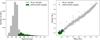 |
Fig. 1. Spectral-type distribution (left) and mass-radius diagram (right) for our 40 pc ML-dwarfs catalogue. In gray: Gaia-2MASS 40 pc sample for late-type stars. In green: SPECULOOS targets (see Sect. 3). |
Our final goal was to build the target list of SPECULOOS using a consistent target selection method, rather to present a complete sample of late-type stars. Therefore, we did not try to recover stars earlier than M6 that were absent from our catalogue because they do not have a Gaia DR2 parallax. Extrapolating our results for ultracool dwarfs to earlier M-dwarfs, we estimate that there must be, at most, a few hundreds of them. To estimate the number of stars that were still missed by our selection process, we derived the number density of stars per cubic parsec. For the early M-dwarf sample (M0 to M5), we derived a distance independent number density of (46.6 ± 0.8) × 10−3 pc−3.
Figure 2 shows the number density for the late M-dwarfs and BDs of our 40 pc sample. We see a lower density for targets closer than 15 pc. This is mainly due to a few nearby stars that are not covered by the Bardalez Gagliuffi et al. (2019) survey and have missing parallaxes in Gaia DR2. For M6 to M7 stars, we derive a distant independent number density between 10 and 40 pc of (3.4 ± 0.2) × 10−3 pc−3. Assuming a homogeneous distribution, we conclude that this sample, as well as our early M-dwarf sample are distance limited with no or negligible brightness selection. For late UCDs with spectral types M8 to L2, we see a drop for targets between 30 and 40 pc, which can be explained by a selection effect that leads to a lack of stars in the order of 102, mostly due to their faintness or crowding in the galactic plane. Finally, for BDs with spectral types later than L2, we see a steep drop with distance. The number density of BDs in our sample decreases by 50% between 10 and 15 pc. This lack of BDs is expected due to the intrinsic faintness of those objects and the limiting magnitude of Gaia (Reylé 2018; Smart et al. 2019).
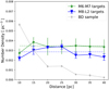 |
Fig. 2. Number densities per distance for different spectral types. Green asterisks: M6 and M7 sub-types; blue triangles: M8 to L2 sub-types; and gray points BDs with types later than L2. The horizontal lines mark the average densities. |
Within 25 pc, we find 214 targets with a photometric spectral type between M6.5 to L0, corresponding to a mean number density of (3.2 ± 0.3) × 10−3 pc−3. This value is about 25% lower than the raw volume-corrected value derived by Bardalez Gagliuffi et al. (2019) ((4.1 ± 0.3) × 10−3 pc−3). This absolute difference can be explained by our selection method, which excludes (i) most close binaries and (ii) blended stars.
3. Observing programmes
As described in Sect. 1, the core science cases of the SPECULOOS survey can be broken down into two major components: (1) a search for transiting, rocky planets that are well-suited for atmospheric characterisation with future facilities, and (2) a statistical census of temperate planets around UCDs. To optimise these goals, we divided the survey into three non-overlapping programmes.
Anticipating the launch of JWST3, we focus in our first programme on a census of targets for which the atmospheric properties of an ‘Earth-like’ planet could be studied in some detail by an ambitious JWST transit spectroscopy observation (Gillon et al. 2020). To qualify as ‘Earth-like’, we denote a planet with the same mass, same size, same atmospheric composition, and same irradiation from the host star as the Earth. Our second programme focuses on a census of temperate rocky planets in the overlapping region between SPECULOOS and TESS in the M5-M6 spectral range. As temperate, we denote a planet that receives four times the irradiation the Earth receives from the Sun, similarly to TRAPPIST-1b. This irradiation is as a boundary, with equilibrium temperatures low enough to allow habitable regions on such tidally locked planets Menou (2013). In this spectral type range, TESS has a declining sensitivity to Earth-sized planets due to a lack of photons, while the SPECULOOS detection efficiency is decreased by the larger periods of temperate planets (relative to later M-dwarfs) that extends the telescope time required per target. A synergetic approach combining the long and continuous observations of TESS and the higher photometric precision of SPECULOOS could thus make detections easier, which would otherwise be difficult to achieve individually. Our third programme focuses on a statistical search for transiting exoplanets within all remaining targets. The criteria to select the targets of the three programmes from our 40 pc list are presented in the following subsections.
3.1. Programme 1: ‘Earth-like’ planets for JWST
To set up the target list of our first programme, we computed the typical S/N achievable in transit transmission spectroscopy by a 200 h observation with JWST/NIRSPEC for all 14 168 objects within our 40 pc sample. Our aim here is to efficiently probe the atmospheric properties of an ‘Earth-like’ planet. For the typical amplitude of the transmission signals, we used the following equation (Winn 2010):
 (4)
(4)
where H is the atmospheric scale height. To derive H, we assume an ‘Earth-like’ planet with the same atmospheric composition as the Earth, an isothermal atmosphere with a mean molecular mass of 29 amu, and a temperature equal to the equilibrium temperature of the planet (with an Bond albedo of 0.3 and irradiation of 1 S⊕). Here, δ is the transit depth and R⊕ is the Earth’s radius. We assumed a value of 5 for NH, which is the number of scale heights corresponding to a strong molecular transition. For the assumed planets, the orbital distance corresponding to an ‘Earth-like’ irradiation was computed based on the stellar luminosity, the corresponding orbital period was computed using Kepler’s third law combined with the stellar mass estimate, and the duration of a central transit was computed using Eq. (15) from Winn (2010). Then, we computed the JWST/NIRSPEC (Prism mode) noise at 2.2 μm for a spectral bin of 100 nm and for an exposure sequence with the same duration as the transit using the online tool PandExo (Batalha et al. 2017). We assumed a red noise over a transit timescale of 30 ppm that we added quadratically to the white noise estimate of PandExo. We computed the number of transits observed within the 200 h JWST programme, assuming for each transit observation, a duration equal to the transit duration plus 2.5 h (for pointing, acquisition, plus out-of-transit observation). The noise per transit was then divided by the square root of the number of observed transits. To the result, we quadratically added an absolute floor noise of 10 ppm. In the end, we obtained, for each target, a transmission S/N by dividing the transmission amplitude by the global noise. Figure 3 (left) shows the resulting SpT−S/N distribution. In this figure, we draw a line at S/N = 4, assuming this value to be an absolute minimum for deriving meaningful constraints on the atmospheric composition of our assumed ‘Earth-like’ planets. TRAPPIST-1 is shown as a magenta star symbol in the figure. For the majority of the targets in the whole 40 pc sample, the achievable S/N is ∼1.
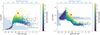 |
Fig. 3. SPECULOOS programme selection: Left: estimated S/N in transmission spectroscopy with JWST/NIRSPEC (assuming an ‘Earth-like’ planet, 200 h of JWST/NIRSPEC time, and a spectral sampling of 100 nm) as a function of spectral type for the 14 164 M- and L-dwarfs within 40 pc. TRAPPIST-1 is shown as a magenta star. Red dashed line: S/N = 4, used to select Programme 1 targets. Colour coding: estimated S/N for detecting a single transit of an Earth-sized planet with one telescope of the SPECULOOS network, with yellow points representing a S/N ≥ 15. Light-blue histogram: distribution of all objects and their corresponding S/N. Right: estimated S/N for TESS to detect an Earth-sized planet with an irradiation four times larger than Earth. Colour coding: estimated S/N for detecting the transit of an Earth-sized planet with the SPECULOOS network, with yellow points representing a S/N ≥ 15. Red dashed line: S/N = 5, used to select Programme 2 targets. Light-blue histogram: distribution of all objects and their corresponding S/N. |
We find that 366 objects – including TRAPPIST-1 – have a S/N ≥ 4, and only 44 of them have a S/N larger than TRAPPIST-1. These 366 objects constitute the target list of SPECULOOS Programme 1. Of the 366, 92 have a spectral type earlier than M6 (and none of them is earlier than M4). We choose to also include these earlier targets in our target list even if they are not bona fide UCDs.
3.2. Programme 2: Temperate, rocky planets from TESS
We set up the targets for our second programme by identifying the synergetic region between SPECULOOS and TESS within our 40 pc sample. For this, we derived first the detection threshold for a temperate, Earth-sized planet for both surveys. For these purposes, we assumed a planet still to be temperate when it receives four times the irradiation the Earth receives from the Sun.
First, we estimated the photometric precision that should be achieved by TESS within 30 min for each object. For this, we adopted the moving 10th percentile of the TESS rms in one hour, as function of the T magnitude, published in Fig. 6 of the TESS Data Release Notes NASA/TM-2018-0000004, assuming the T magnitude to be similar to the Ic magnitude, derived earlier. This rms was multiplied by the square root of two to get the rms in 30 min. Then, we assumed for each target an Earth-sized planet on a close-in orbit (receiving an irradiation of four times that of Earth) and computed the detection S/N expected from two 27 d observations with TESS. For the noise of the TESS observations, we took into account the mean number of observed transits during the observation, their depths, durations (assuming a central transit), as well as our estimate for the TESS photometric precision for the star. Furthermore, we assumed a floor noise of 50 ppm per transit, and no noise for the phase-folded photometry. If the computed S/N was ≥5, a detection within the reach of TESS was inferred.
We applied the same procedure for SPECULOOS. First, we used the SPECULOOS Exposure Time Calculator to compute the typical photometric precision for each target that should be achieved by a SPECULOOS 1 m-telescope in the I + z filter (Delrez et al. 2018b) as a function of the apparent J-band magnitude and the spectral type of the target. A detailed discussion on the typical noise achieved for SPECULOOS targets with our 1 m telescopes is given in Murray et al. (2020). To simulate this typical noise by using the SPECULOOS Exposure Time Calculator, we assumed a 100 h-long photometric monitoring and an average floor noise of 500 ppm per transit. Here too, a detection was deemed possible when the computed S/N was ≥5.
Figure 3 (right) shows a summary of our results. For our 40 pc sample, the detection S/N with TESS for temperate, rocky planets increases for earlier M-dwarfs due to its excellent time coverage and the decreasing orbital periods for temperate planets with increasing spectral type. Nevertheless, it greatly decreases at spectral type ∼M5 due to the faintness of the objects, which is in line with Sullivan et al. (2015). The colour coding shows the S/N achieved by SPECULOOS for the same temperate planets. The S/N starts to increase at spectral type ∼M5 towards later spectral types due to its shorter monitoring strategy (for most earlier-type objects, only one transit can be observed in 100 h), but its smaller photon noise compared to TESS.
In this context, for the second programme (hereafter, Programme 2), we selected stars with photometric spectral types M5 and later, for which Earth-sized planets with an irradiation that is four times that of Earth can be detected by TESS with a S/N ≥ 5. These criteria are met for some targets previously selected in our Programme 1. Thus we apply those criteria to select stars from our 40 pc sample that are not in Programme 1.
The target list of Programme 2 ultimately contains 171 objects that have spectral types mainly between M5V and M6.5V. For these targets, we aim to identify low-significance (5 to 8 sigma) transit signals of Earth-sized planets in TESS photometry first, which are then observed with SPECULOOS to confirm or discard their planetary nature (see details in Sect. 5.2).
3.3. Programme 3: The SPECULOOS statistical survey
The third programme (hereafter, Programme 3) is the SPECULOOS statistical survey. It focuses on all objects from our target list not covered by the two first programmes, including all UCDs (later than M6) from our 40 pc sample. Given the uncertainty of our classification, we selected all objects with photometric classifications of M6 and later to ensure the inclusion of all UCDs. This programme contains 1121 targets.
4. Catalogue characterisation and new targets
The full SPECULOOS input catalogue is composed of all targets from three programmes described above. To characterise the sample, we cross-matched our catalogue with known objects in the literature. As there is no complete database for all UCDs available so far, we carried out our cross-check with multiple catalogues and databases. The most comprehensive database so far is SIMBAD (Wenger et al. 2000). It lists spectroscopic classifications for 44% of our targets. Further catalogues, which we used for the cross-check were: DwarfAchives.org5, the compilation by J. Gagné6, the list published by Kiman et al. (2019) and compiled from the BOSS ultracool dwarf survey, the compilation from Bardalez Gagliuffi et al. (2019), as well as the compilations from Smart et al. (2019), Reylé (2018), and Scholz (2020) based on Gaia DR2. When spectral types from optical and infrared spectra were given, we adopted the spectral type derived from the optical spectrum first and only adopted the infrared spectral type if no optical spectrum was obtained. When a spectral type or catalogue entry was derived from photometry only, we denoted this entry as a photometric spectral type. When the origin of a spectral classification cannot be verified (for example, when a reference is missing in SIMBAD), we denoted this entry as a photometric spectral type as well.
We rejected the object 2MASS J10280776−6327128 from our catalogue, as it is a known white dwarf (Kirkpatrick et al. 2016). Another three targets were rejected because they are classified as subdwarfs, namely, 2MASS J02302486+1648262 (Cruz & Reid 2002), 2MASS J14390030+1839385 (Gizis 1997), and 2MASS J17125121−0507249 (Aganze et al. 2016). Finally, we ended up with a catalogue of 1657 SPECULOOS targets.
Table 1 shows the list descriptions for the online table. It contains all SPECULOOS targets, their derived parameters as described in Sect. 2, as well as the spectral types available in literature. We find that 50% have spectral types in literature, 28.1% have photometric spectral types only, and 21.9% (363 targets) have been classified in this work for the first time (shown in Table 3). The majority of them (260 targets) are classified as M6 and later. Taking into consideration the uncertainties from our photometric classification, we refer to those targets as potential ‘new’ UCDs.
Column description of the SPECULOOS target list.
Newly classified low-mass stars and brown dwarfs from the SPECULOOS input catalogue.
The spectral type distribution of the SPECULOOS catalogue peaks at M6V with about 400 targets and decreases with later spectral types. As shown in Fig. 1, the catalogue is incomplete for targets earlier than M6V because of the varying spectral type cut of the different programmes. Nevertheless, no cuts were introduced for later-type stars. In Fig. 4, we show the distribution of UCDs within catalogue (photometric spectral type M6V or later) and the corresponding coverage with literature spectral types. We note an apparent lack of spectral classifications for earlier-type objects, while the sample is almost complete for BDs. This bias is in line with the findings from Reylé (2018). It mostly originates from intensive spectral typing of the BD sample in the past decade.
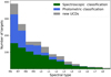 |
Fig. 4. Distribution of photometric spectral types for UCDs within 40 pc from the SPECULOOS input catalogue. Colour coding: targets with spectroscopic classification (green), with photometric classification (blue); and newly identified UCDs without spectral type in the literature (gray). |
We compared our photometric spectral types (derived as described in Sect. 2) to spectroscopic measurements for the 829targets for which we found a spectroscopic classification in the literature. We found that the photometric classification agrees best for the M-dwarf stars in our sample with an average difference below one sub-class. For later objects and brown dwarfs, we found that the photometric classification is on average one sub-class earlier than the spectroscopic classifications. The results of the comparison are shown in Table 2.
Comparison between photometric and spectroscopic classifications.
5. Observing strategy
5.1. SPECULOOS monitoring strategy
The basic observational strategy of SPECULOOS is to observe each target continuously with one telescope for a duration that is long enough to capture the observation of at least one transit of a temperate planet. Therefore, we observed one or two targets per night with each telescope. Other surveys have proceeded differently (Nutzman & Charbonneau 2008; Tamburo & Muirhead 2019), but considering our requirement for very-high photometric precision and the expected short transit duration (down to 15 min) for very-short-period (≤1 d) planets orbiting UCDs, we estimate that a continuous observation approach is more appropriate (Delrez et al. 2018a; Gibbs et al. 2020).
Considering that we have divided our target list in three distinct programmes, the SPECULOOS observing strategy is also divided into three. For instance, Programme 1 is aimed at performing a more complete coverage of the habitable zone of its targets than Programmes 2 and 3 and so, its monitoring duration per target has to be more extensive than for the two other programmes.
Up until Nov. 2019, our strategy was the same for all programmes, with a monitoring duration of 100 h for any target no matter which programme it belongs to (that is to say, stars were observed until 100 h of photometric data have been gathered). Furthermore, we used to split the observation for each target into two observation blocks of each 50 h per year. Our intention back then was to survey many targets to detect quickly very-short-period planets, which would enable us to trigger intensive follow-up to detect additional planets (if present) with larger periods in the system. However, we have now settled on a different strategy: a monitoring duration of 200 h in one block for the target of Programme 1 and a duration of 100 h in one block for the targets of Programmes 2 and 3.
To ensure we picked the most appropriate strategy for the three SPECULOOS observation programmes, we used a metric that we call the effective phase coverage. This metric gives an estimation of how the phase of an hypothetical planet would be covered for a range of periods, using existing observations from the SPECULOOS network. More precisely, we computed the percentage of phase covered for each orbital period from P = 0.1 d to P = Pmax and took the effective phase coverage for periods ≤Pmax to be the integral over the period range. Figure 5 shows the phase coverage for each possible orbital period for an arbitrary target observed for 134.3 h by SPECULOOS. The effective phase coverage is depicted by the blue area, for Pmax = 6 d.
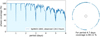 |
Fig. 5. Left: phase coverage as a function of the orbital period of an hypothetical planet around the target pcrSp0643-1843 (chosen arbitrarily), observed for 134.3 h in total by SPECULOOS. Right: graphic visualisation of the coverage of target pcrSp0643-1843 for an orbital period of 4.7 days. Each blue circular arc represents one night of observation; its size is proportional to the number of hours observed each night and the full circle depicts a duration of 4.7 days. |
In the next sections, we detail how this metric drives our programme-specific strategy.
5.1.1. Strategy of Programmes 2 and 3
Programmes 2 and 3 focus on the detection of planets with irradiations similar to TRAPPIST-1b (4 S⊕) and, thus, with short orbital periods. To ensure that we cover all short-period planets, we set Pmax = 6 d and calculated the effective phase coverage for all targets for which observations with the SPECULOOS network have been initiated. Additionally, we performed simulations of SPECULOOS observations, assuming four hours of observations per night per target and losses (bad weather or full moon too close) of 30%.
Figure 6 shows the evolution of the effective coverage as a function of the number of hours surveyed for all periods ≤Pmax = 6 days. We observe that for 50 h of observationsm the expected phase coverage is 60%, whereas for 100 h of observations it increases to 80%. The SPECULOOS data agree well with our simulations and show that for our targets in Programmes 2 and 3, a monitoring duration of 100 h will allow us to detect close-in planets with an effective phase coverage of more than 80%. Figure 6 also shows the number of targets for which observations have started as a function of the coverage. We see that the majority of these targets have been covered at 60−70% for periods going from 0.1 to 6 days. This is explained by the fact that for many targets, we had already gathered more than 50 h during the first year of observations.
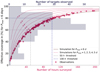 |
Fig. 6. Effective coverage as a function of the number of hours surveyed for all targets observed by the SPECULOOS telescopes so far. Coloured dots shows the coverage calculated from existing observation, for periods going from 0.1 to 6 days. The solid red line is the corresponding simulation. Dashed red lines are simulations for various values of Pmax ranging from one to five days. Gray histogram: number of targets in each slice of coverage. |
To analyse the effect of splitting the 100 h observations into two blocks of 50 h per year, we compared the effective phase coverage for two SPECULOOS targets that have both been monitored with SPECULOOS for 100 h, but with the two different strategies. Figure 7 shows the phase coverage for each possible orbital period for both targets. We also show simulated SPECULOOS observations for comparison.
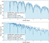 |
Fig. 7. Top: evolution of the phase coverage as a function of the period for one SPECULOOS target (pcrSp0306-2647) observed for 100 h with SSO in two blocks of 50 h several months apart. The solid blue line shows the evolution of the coverage calculated from existing observations whereas the gray line is the result of simulations. Bottom: same for another SPECULOOS target (pcrSp0306-3647) observed 100 h with SSO but on consecutive days. |
In the first scenario, the target was observed for 50 h on consecutive days, and again 50 h one year later (top panel of Fig. 7), whereas in the second scenario, the target was observed day after day until 100 h of observations were reached (bottom panel of Fig. 7). We found that splitting the observations does a better job of shuffling the phases but this also introduces aliases that result in a slightly decreased coverage for orbital periods close to multiples of sidereal days. As a whole, observations and simulations indicate that the effective coverage is with −0.7 ± 1.4% similar for both scenarios.
More generally, in our simulations, we used a period grid of 15 min which resembles the minimum expected transit duration. We find that between 0.1 and 6 days, about 40% of all possible orbital periods gain phase coverage from continuous observations, compared to 20.0% that lose coverage. Despite similar effective phase coverage, for about 20% (30% for planets with 8−12 d period) of all possible orbital periods, we find a better phase coverage for continuous observations with SPECULOOS.
Additionally, given the continuous observation strategy is also more straightforward from the scheduling point of view, we opted to observe each target without additional splitting until its programme-specific monitoring duration is reached. In the same way, we expect a slight increase of effective phase coverage of 1.2 ± 0.7% for observations in the case that we can observe a target all night long. We also find an increased phase coverage for about 7% of all possible orbital periods. Thus, we opted to observe each target for the entire night when possible.
5.1.2. Strategy of Programme 1
The objective of our Programme 1 is to detect possible transiting ‘Earth-like’ planets with irradiations similar to Earth (1 S⊕) and, thus, with orbital periods in or close to the habitable zone (HZ) of their host.
Figure 8 shows the effective coverage of the targets of Programme 1 as already initiated with SPECULOOS as a function of the number of hours surveyed. Here, we use as Pmax the middle of the HZ, which has been calculated for each target following Kopparapu et al. (2013). For most of the observed Programme 1 targets, a hypothetical planet in the HZ would have a period of between eight to ten days and would require ≃200 h of observation to reach a coverage ≥80%. Thus, for our targets in Programme 1, a monitoring duration of 200 h will effectively allow us to detect planets in the habitable zone. In addition, the conclusion given in Sect. 5.1.1 (still true for 200 h) asserts that we decided to monitor each target on consecutive days if possible until the monitoring duration has been reached, without splitting the observations between different years.
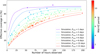 |
Fig. 8. Coverage of the middle of the HZ for the targets of Programme 1 observed so far by the SPECULOOS survey. Solid lines: theoretical simulations, Coloured dots: actual SPECULOOS observations. Colour coding: expected maximum orbital periods associated with the middle of the HZ of each target. |
5.2. SPECULOOS targets observed with TESS
For Programme 2, we selected all objects that would allow for the detection of temperate (namely, with four times the irradiation of the Earth), Earth-sized planets with TESS. This is also the case for many targets in our Programme 1 since, for the earliest-type of them, TESS photometry should be precise enough to enable the detection of short-period planets. For the others, it could at least constrain their photometric variability. Thus, we decided to systematically analyse the TESS photometry in advance (if possible) of our SPECULOOS observations and to ultimately perform a global analysis of the light curves gathered by both surveys so as to maximize the scientific return.
At the time of writing (May 2020), from the targets in our Programmes 1 and 2, there are 231 that have 2 min cadence lightcurves provided by the Science Processing Operations Center (SPOC, Jenkins et al. 2016), whereas 167 have only 30 min cadence lightcurves from full frame images, and 138 are scheduled for observations with TESS. None of the targets observed have been issued an alert from the automatic pipelines of TESS. This hints at a lack of clear transits in the TESS data set.
In order to search for threshold-crossing events that might go unnoticed, we made use of our custom pipeline pcrSHERLOCK7 (Pozuelos et al. 2020; Demory et al. 2020). This pipeline downloads the Pre-search Data Conditioning Simple Aperture (PDC-SAP) flux data from the NASA Mikulski Archive for Space Telescope (MAST) by means of the LIGHTKURVE package (Lightkurve Collaboration 2018). Then, it removes outliers defined as data points > 3σ above the running mean, and removes the stellar variability using WOTAN (Hippke et al. 2019) using two different detrending methods: a bi-weight filter and a Gaussian process with a Matern 3/2-kernel. To optimise the search for transits, the pipeline was run for a number of trials in which the window and kernel sizes are varied for each respective aforementioned method. The transit search is performed by the TRANSIT LEAST SQUARES package (Hippke & Heller 2019), which is optimised for the detection of shallow periodic transits. We set our threshold limits at S/Ns of ≥5 and signal detection efficiencies (SDEs) of ≥5, and followed the in-depth vetting process described by Heller et al. (2019).
For each event that overcomes the vetting process, we performed a ground-based follow-up campaign with our SPECULOOS network to rule out potential sources of false positives and strengthen the evidence of its planetary nature. Given the large pixel size of TESS (21″ pixel−1), the point spread function can be as large as 1′, which increases the probability of contamination due to a nearby eclipsing binary (EB). Indeed, a deep eclipse in a nearby EB may mimic a shallow transit detected for a target star due to dilution. Hence, it is critical to identify potential contamination due to EBs or relatively nearby neighbours up to 2.5 arcmin (e.g. Kostov et al. 2019; Quinn et al. 2019; Günther et al. 2019; Nowak et al. 2020). To schedule photometric time-series follow-up observations, we use the TESS Transit Finder, which is a customized version of the Tapir software package (Jensen 2013), in coordination with the SPECULOOS scheduler described in Sect. 6.
For the analysis of a given candidate that yields negative results, we may wonder if the photometric precision of the TESS lightcurve is high enough to confidently rule out the presence of Earth-sized planets in the habitable zone. To check the detectability of such planets in the TESS data set, we performed an injection-and-recovery test. This consists of injecting synthetic planetary signals into the PDC-SAP flux light curve before the detrending and the transit search stages described above. We explore the Rplanet − Pplanet parameter space in the ranges of 0.7−2.7 R⊕ with steps of 0.05 R⊕, and 1−x d with steps of 0.5 d, where x is the largest period for a planet residing in the habitable zone of the given candidate (Kopparapu et al. 2013). For example, for the TRAPPIST-1 system, x ∼ 15 d, indicating an exploration of periods ranging from 1 to 15 d, which combined with a radius range of (0.7−2.7 R⊕) consists of 1189 different scenarios. A graphical example is shown in Fig. 9 for one of our candidates in Programme 1, which yielded a negative result in the previous search for threshold-crossing events. If, following all these analyses, we cannot firmly rule out the presence of Earth-sized planets orbiting the habitable zone of a given star on our list, we plan to observe it for 100 h with the SPECULOOS network.
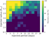 |
Fig. 9. Graphical example of the inject-an-recovery test performed for one of our candidates in Programme 1 (Sp0025+5422). The Rplanet − Pplanet parameter space explored corresponds to a planetary radius range of 0.7−2.7 R⊕ with steps of 0.05 R⊕, and a period range of 1−19 d with steps of 0.5 d. This yields a total of 1517 scenarios. The recovery rate is presented by the colour coding. Planets smaller than 1.4 R⊕ would remain undetected for almost the full set of periods explored. |
6. The SPECULOOS scheduler
In order to handle the three different programmes and optimise the visibility windows of our 1657 targets, we developed a planification tool, named the SPeculoos Observatory sChedule maKer (pcrSPOCK. All SPECULOOS observatories are controlled using the commercial software ACP8, thus, its primary aim is to prepare daily observing scripts (ACP plans) for the SSO, SNO, and SAINT-EX observatories (source code available on Github9).
In order to decide which targets to observe, pcrSPOCK relies on the priority and observability of each target. The priority is essentially defined as the value of the S/N for JWST transmission spectroscopy for an ‘Earth-like’ planet in Programme 1, the TESS detection S/N for a temperate planet in Programme 2 and the SPECULOOS detection S/N for a temperate planet in Programme 3. The observability is computed as the best visibility window of the year for each target. Every time a schedule is made, SPOCK selects new targets that are at their optimum visibility at this time of the year. The selected targets are then ranked and the one with the highest priority is scheduled (providing it respects constraints imposed by the facility such as moon distance and altitude). When observable all night, the target is simply scheduled all night, but if some gaps remain, an additional target is added to complement the schedule and avoid losing observing time. Furthermore, to prevent having overly short observation blocks (1 h or less), the duration of the two targets are set to be comparable. For instance, if one night is 8 h long and target 1 is observable for the first 7 h only, target 2 is not going to be scheduled for the last hour only but rather the night will be split in half such that target 1 and 2 are observed for approximately the same amount of time. We say approximately because we do not exactly split the night in half; instead, we adopt a nightly observing duration adapted to each target’s visibility, which will shift from night to night during the observation period. This situation of observing two targets per night rather than one can happen frequently, as many targets have latitudes that do not allow for all the available night time for the given site to be filled up – even at their peak of visibility. As a whole, we can make the assumption that a night lasts 8 h and we can approximate that the duration of the observation for each target is 4 h, which justifies our use of observation blocks of 4 h in the simulations detailed in Sect. 5.1.
To implement those constraints, pcrSPOCK makes use of the pcrASTROPLAN package (Morris et al. 2018), which is a flexible Python toolbox for astronomical observation planning and scheduling. pcrSPOCK also optimises the choice of the period of the year for which the target is the most visible at a relatively low airmass, based on the completion ratio of the target and the optimisation of available observatories. The completion ratio is defined as  , which embodies the fraction of hours of observation completed versus the number of hours required for each target. We note that the value of hoursthreshold depends on the programme the target belongs to, namely, 200 h for Programme 1 and 100 h for Programmes 2 and 3. Using this completion ratio to rank targets is useful for favouring the quick completion of ongoing targets, as opposed to starting new ones continually. As SPECULOOS is an all-sky survey, one of the main roles of pcrSPOCK is to handle the coordination of multi-site observations. For instance, between two targets with similar priorities but one observable only from one site and the other from several sites, pcrSPOCK will choose the target that yields the most coverage. In addition, when possible, a one-hour overlap between observations from two different sites is scheduled to aid in the recombination of the light curves.
Figure 10 shows the targets scheduled so far by pcrSPOCK. As explained in Sect. 5, the former strategy of dividing the observations in blocks of 50 h was prevalent until recently (Nov. 2019). Therefore, many targets are currently in the ‘ongoing observation’ phase. We note that observations have started for more than half of Programme 1 targets (S/NJWST ≥ 4).
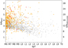 |
Fig. 10. Estimated S/N as a function of spectral type. Gray dots represents all targets in the SPECULOOS target list, orange dots stand for targets for which observations have been initiated but not completed, and red dots stand for completed targets (i.e. observed for 200 h if the target is in Programme 1 and for 100 h if the target is in Programme 2 or 3). |
7. Updated planet yield for SPECULOOS
In Delrez et al. (2018a; hereafter, D18), we simulated the planet yield expected from the SPECULOOS survey, assuming a total observation of 100 h per target. We updated this simulation in order to include the SPECULOOS target list presented in this paper. Also, we accounted for the physical parameters that were derived for each target.
To estimate the planet detection yield, we used a Monte Carlo simulation that looped 1000 times over the target sample. First, we assumed that every target has at least one planet and used the mass, radius, and effective temperature as starting points to simulate a planetary system. To account for the errors in stellar parameters, in each loop, we drew the simulated mass, radius, and effective temperature from a normal distribution with μ = parameter and σ = error of parameter.
Secondly, for each target, we drew a planetary system following Miguel et al. (2020), using their distribution of expected number of planets. We accounted for the period distribution by using two period samples, one between 0.5 and 23 days and a second between 23 and 1800 days. The drawn planets are uniformly distributed with a probability of p = 0.5 to be in one of both samples. The planet masses and densities are drawn from a normal distribution based on the TRAPPIST-1 system with:
-
Planetary mass (M⊕) N(0.81, 0.342).
-
Planetary density (ρ⊕) N(0.79, 0.122).
We derived the planet parameters and inclinations based on the stellar parameters using the same methods as described in D18. Simulated planets are counted as ‘discovered’ if the following criteria are met: (1) a transit has been observed during a simulated SPECULOOS observation run. This assumes a visibility of 4 h per night, a total loss of about 30% due to weather or technical downtime, and a monitoring campaign that is completed after the programme-specific number of observing hours has been reached; (2) the S/N of the transit is larger than 5, assuming a floor noise during the transit of 500 ppm.
From this simulation, we derived: (i) the number of planets detected during the SPECULOOS observation windows; (ii) how many of them are, in fact, transiting systems (having more than one transiting planet); and (iii) how many of them are in the habitable zone. We denote a simulated planet as being in the habitable zone if the received incident flux meets the criterion: 0.2 < S⊕ < 0.8, which resembles the conservative limits derived by Kopparapu et al. (2013).
Table 4 summarises the results for the three SPECULOOS sub-programmes, as well as the results from D18 for comparison. For the complete SPECULOOS programme, with all observing programmes completed, we expect 29 ± 4 planets, with 8 ± 2 of them being in the habitable zone of their host star. The changes to our expectation from D18 are mainly due to the different simulated system architectures. In D18, we assumed about the same number of planets, but distributed within a period range extending only to 23 d. Planets with large periods are less likely to be transiting. For the D18 expectation, about 1.8% of all planets were transiting, while we now find a fraction of 0.9% of transiting planets. Furthermore, SPECULOOS is by design less sensitive to planets with long periods. We find that 6.5% of all targets with at least one transiting planet host seven or more planets (0.5% for Kmag < 10.5). Given the expected number of detections, we conclude that the detection by SPECULOOS of a ‘better’ system than TRAPPIST-1 (in terms of atmospheric follow-up potential) is very unlikely.
Expected planet yield from the SPECULOOS survey.
At the time of writing (May, 2020), we monitored about 10% of all SPECULOOS targets for more than 50 h. Applying our simulation to this sub-sample, we would expect about 2 ± 2 planets to be discovered in the survey by now, which is consistent with TRAPPIST-1 standing as the only such detection thus far.
8. Summary and conclusions
In this work, we present the SPECULOOS target list containing 1657 very-low-mass dwarfs within 40 pc. We derived photometric classifications and stellar properties for each target.
Our target selection procedure is based on a cross-match between Gaia DR2 and 2MASS catalogues, not only in terms of astrometric position but also in terms of inferred spectral type. We show that our sample is indeed volume limited for UCDs with spectral type earlier than M8, which includes the brightest UCDs and thus the most promising targets to search for terrestrial planets, suitable for atmospheric characterisation. The rationale of our target selection is to minimize the false positive rate, which is important, as about 50% of our targets lack a spectroscopic classification and only a few of the spectroscopically classified targets have been identified as false positives like white dwarfs or subdwarfs. The SPECULOOS target list includes targets with photometric spectral types from M4 to L9. 363 targets have not been classified in the literature so far, with 260 of them having photometric spectral types of M6V and later. Including the uncertainties of our classification, we denote those targets as potential ‘new’ UCDs.
The main goals of the SPECULOOS project are (1) to detect ‘Earth-like’ planets that are perfectly suited for atmospheric characterisation with JWST and (2) to draw constraints to the structure of planetary systems of UCDs by surveying our volume-limited sample of UCDs for exoplanet transits.
To optimise the scientific return of the project, we divided it into three, non-overlapping observation programmes: Programme 1, which includes all targets that allow transit transmission spectroscopy with JWST for ‘Earth-like’ (irradiation of 1 S⊕) planets (365 targets); Programme 2, which includes all targets that allow a detection of Earth-sized temperate (irradiation of 4 S⊕) planets – like TRAPPIST-1b – with TESS (171 targets); and Programme 3, which includes all other SPECULOOS targets with spectral type M6 and later and aims to explore the planet occurrence rate for ultracool dwarfs within our 40 pc sample (1121 targets). From all targets in Programme 1, we expect only 44 of them to have a higher S/N than for the TRAPPIST-1 planets. This underlines the unique nature of this system and its importance for atmospheric characterisation of ‘Earth-like’ planets.
Our strategy is to observe all targets, reaching an effective phase coverage of up to 80% for temperate planets in Programmes 2 and 3 and for planets in the habitable zone in Programme 1, resulting in monitoring durations with our SPECULOOS telescope network of 100 to 200 h, respectively. To optimise the survey, we leverage on the synergy with TESS by analysing TESS data for all targets in our Programmes 1 and 2 that also: (1) have been observed by the TESS mission; and (2) are bright enough that we can discover temperate Earth-sized planets in TESS.
Furthermore, we derived the expected planet yield from the SPECULOOS survey, using a Monte Carlo simulation based on our target list and observation programs. Given our observational strategy, we expect SPECULOOS to detect a few dozen planets, including up to a dozen potentially habitable ones. We also find that with SPECULOOS, we should have already found 2 ± 2 planets, among our targets. Within the errors, this is consistent with our current lack of detections, apart from TRAPPIST-1. Given its focus on Earth-sized planets in a volume limited all-sky sample of UCDs, the detection rate inferred from the SPECULOOS survey will allow us to draw robust constraints to the structure of planet systems of UCDs.
As 50% of our targets had not yet been spectroscopically classified in literature at the time of this study, a large-scale spectroscopic follow-up program will be necessary in order to: (1) improve our photometric spectral classification and (2) exclude potential false classifications. The upcoming Gaia DR3 release will largely improve the parallaxes and colours for the 40 pc sample, thus encompassing more targets that were excluded in this paper. We plan to use our target selection algorithm to further identify nearby targets once the next release becomes available.
We used the BCJ(SpT) relationship of F2015 (assumed internal error = 0.163), and for stars earlier than SpT M6.64 (selected so to ensure the continuity of the two laws), we used the BCJ(Teff) relationship of PM2013 assuming an internal error of 0.2.
SHERLOCK (Searching for Hints of Exoplanets fRom Lightcurves Of spaCe-based seeKers) code is available upon request.
Acknowledgments
The research leading to these results has received funding from the European Research Council (ERC) under the European Union’s Seventh Framework Programme (FP/2007–2013) ERC Grant Agreement n° 336480, from the ARC grant for Concerted Research Actions financed by the Wallonia-Brussels Federation, from the Balzan Prize Foundation, and from F.R.S.-FNRS (Research Project ID T010920F). MG is F.R.S.-FNRS Senior Research Associate. This research is also supported work funded from the European Research Council (ERC) the European Union’s Horizon 2020 research and innovation programme (grant agreement n° 803193/BEBOP), from the MERAC foundation, and through STFC grants n° ST/S00193X/1 and ST/S00305/1. B.V.R. thanks the Heising-Simons Foundation for Support. This work has made use of data from the European Space Agency (ESA) mission Gaia (https://www.cosmos.esa.int/gaia), processed by the Gaia Data Processing and Analysis Consortium (DPAC, https://www.cosmos.esa.int/web/gaia/dpac/consortium). Funding for the DPAC has been provided by national institutions, in particular the institutions participating in the Gaia Multilateral Agreement. This publication makes use of data products from the Two Micron All Sky Survey, which is a joint project of the University of Massachusetts and the Infrared Processing and Analysis Center/California Institute of Technology, funded by the National Aeronautics and Space Administration and the National Science Foundation. This research has made use of the SIMBAD database, operated at CDS, Strasbourg, France, This research has made use of the VizieR catalogue access tool, CDS, Strasbourg, France. This research made use of Astropy (http://www.astropy.org), a community-developed core Python package for Astronomy (Astropy Collaboration 2013, 2018).
References
- Aganze, C., Burgasser, A. J., Faherty, J. K., et al. 2016, AJ, 151, 46 [NASA ADS] [CrossRef] [Google Scholar]
- Alibert, Y., & Benz, W. 2017, A&A, 598, L5 [NASA ADS] [CrossRef] [EDP Sciences] [Google Scholar]
- Astropy Collaboration (Robitaille, T. P., et al.) 2013, A&A, 558, A33 [NASA ADS] [CrossRef] [EDP Sciences] [Google Scholar]
- Astropy Collaboration (Price-Whelan, A. M., et al.) 2018, AJ, 156, 123 [Google Scholar]
- Barclay, T., Pepper, J., & Quintana, E. V. 2018, ApJS, 239, 2 [NASA ADS] [CrossRef] [Google Scholar]
- Bardalez Gagliuffi, D. C., Burgasser, A. J., Schmidt, S. J., et al. 2019, ApJ, 883, 205 [NASA ADS] [CrossRef] [Google Scholar]
- Batalha, N. E., Mandell, A., Pontoppidan, K., et al. 2017, PASP, 129, 064501 [NASA ADS] [CrossRef] [Google Scholar]
- Benneke, B., Wong, I., Piaulet, C., et al. 2019, ApJ, 887, L14 [NASA ADS] [CrossRef] [Google Scholar]
- Berta-Thompson, Z. K., Irwin, J., Charbonneau, D., et al. 2015, Nature, 527, 204 [NASA ADS] [CrossRef] [PubMed] [Google Scholar]
- Burdanov, A., Delrez, L., Gillon, M., & Jehin, E. 2018, SPECULOOS Exoplanet Search and its Prototype on TRAPPIST, 130 [Google Scholar]
- Burgasser, A. J., Gillon, M., Melis, C., et al. 2015, AJ, 149, 104 [NASA ADS] [CrossRef] [Google Scholar]
- Charbonneau, D., Berta, Z. K., Irwin, J., et al. 2009, Nature, 462, 891 [NASA ADS] [CrossRef] [PubMed] [Google Scholar]
- Coleman, G. A. L., Leleu, A., Alibert, Y., & Benz, W. 2019, A&A, 631, A7 [NASA ADS] [CrossRef] [EDP Sciences] [Google Scholar]
- Crossfield, I. J. M., Waalkes, W., Newton, E. R., et al. 2019, ApJ, 883, L16 [CrossRef] [Google Scholar]
- Cruz, K. L., & Reid, I. N. 2002, AJ, 123, 2828 [NASA ADS] [CrossRef] [Google Scholar]
- Cruz, K. L., Reid, I. N., Liebert, J., Kirkpatrick, J. D., & Lowrance, P. J. 2003, AJ, 126, 2421 [NASA ADS] [CrossRef] [Google Scholar]
- de Wit, J., & Seager, S. 2013, Science, 342, 1473 [NASA ADS] [CrossRef] [Google Scholar]
- Delrez, L., Gillon, M., Queloz, D., et al. 2018a, in SPIE Conf. Ser., Proc. SPIE, 10700, 107001I [Google Scholar]
- Delrez, L., Gillon, M., Triaud, A. H. M. J., et al. 2018b, MNRAS, 475, 3577 [NASA ADS] [CrossRef] [Google Scholar]
- Demory, B.-O., Gillon, M., Madhusudhan, N., & Queloz, D. 2016, MNRAS, 455, 2018 [NASA ADS] [CrossRef] [Google Scholar]
- Demory, B.-O., Pozuelos, F. J., Gómez Maqueo Chew, Y., et al. 2020, A&A, 642, A49 [CrossRef] [EDP Sciences] [Google Scholar]
- Dieterich, S. B., Henry, T. J., Jao, W.-C., et al. 2014, AJ, 147, 94 [NASA ADS] [CrossRef] [Google Scholar]
- Dittmann, J. A., Irwin, J. M., Charbonneau, D., et al. 2017, Nature, 544, 333 [NASA ADS] [CrossRef] [Google Scholar]
- Filippazzo, J. C., Rice, E. L., Faherty, J., et al. 2015, ApJ, 810, 158 [Google Scholar]
- Gaia Collaboration (Prusti, T., et al.) 2016, A&A, 595, A1 [NASA ADS] [CrossRef] [EDP Sciences] [Google Scholar]
- Gaia Collaboration (Brown, A. G. A., et al.) 2018, A&A, 616, A1 [NASA ADS] [CrossRef] [EDP Sciences] [Google Scholar]
- Gibbs, A., Bixel, A., Rackham, B. V., et al. 2020, AJ, 159, 169 [CrossRef] [Google Scholar]
- Gillon, M. 2018, Nat. Astron., 2, 344 [NASA ADS] [CrossRef] [Google Scholar]
- Gillon, M., Jehin, E., Magain, P., et al. 2011, Eur. Phys. J. Web Conf., 11, 06002 [Google Scholar]
- Gillon, M., Jehin, E., Fumel, A., Magain, P., & Queloz, D. 2013, Eur. Phys. J. Web Conf., 47, 03001 [CrossRef] [Google Scholar]
- Gillon, M., Jehin, E., Lederer, S. M., et al. 2016, Nature, 533, 221 [NASA ADS] [CrossRef] [PubMed] [Google Scholar]
- Gillon, M., Triaud, A. H. M. J., Demory, B.-O., et al. 2017, Nature, 542, 456 [NASA ADS] [CrossRef] [PubMed] [Google Scholar]
- Gillon, M., Meadows, V., Agol, E., et al. 2020, ArXiv e-prints [arXiv:2002.04798] [Google Scholar]
- Gizis, J. E. 1997, AJ, 113, 806 [NASA ADS] [CrossRef] [Google Scholar]
- Günther, M. N., Pozuelos, F. J., Dittmann, J. A., et al. 2019, Nat. Astron., 3, 1099 [Google Scholar]
- Hardegree-Ullman, K. K., Cushing, M. C., Muirhead, P. S., & Christiansen, J. L. 2019, AJ, 158, 75 [NASA ADS] [CrossRef] [Google Scholar]
- Hawley, S. L., Covey, K. R., Knapp, G. R., et al. 2002, AJ, 123, 3409 [NASA ADS] [CrossRef] [Google Scholar]
- He, M. Y., Triaud, A. H. M. J., & Gillon, M. 2017, MNRAS, 464, 2687 [NASA ADS] [CrossRef] [Google Scholar]
- Heller, R., Hippke, M., & Rodenbeck, K. 2019, A&A, 627, A66 [NASA ADS] [CrossRef] [EDP Sciences] [Google Scholar]
- Henry, T. J., Subasavage, J. P., Brown, M. A., et al. 2004, AJ, 128, 2460 [NASA ADS] [CrossRef] [Google Scholar]
- Henry, T. J., Jao, W.-C., Winters, J. G., et al. 2018, AJ, 155, 265 [NASA ADS] [CrossRef] [Google Scholar]
- Hippke, M., & Heller, R. 2019, A&A, 623, A39 [NASA ADS] [CrossRef] [EDP Sciences] [Google Scholar]
- Hippke, M., David, T. J., Mulders, G. D., & Heller, R. 2019, AJ, 158, 143 [NASA ADS] [CrossRef] [Google Scholar]
- Howard, A. W., Marcy, G. W., Bryson, S. T., et al. 2012, ApJS, 201, 15 [NASA ADS] [CrossRef] [Google Scholar]
- Jehin, E., Gillon, M., Queloz, D., et al. 2011, The Messenger, 145, 2 [NASA ADS] [Google Scholar]
- Jehin, E., Gillon, M., Queloz, D., et al. 2018, The Messenger, 174, 2 [NASA ADS] [Google Scholar]
- Jenkins, J. M., Twicken, J. D., McCauliff, S., et al. 2016, in SPIE Conf. Ser., Proc. SPIE, 9913, 99133E [Google Scholar]
- Jensen, E. 2013, Astrophys. Source Code Libr. [record ascl:1306.007] [Google Scholar]
- Kaltenegger, L., & Traub, W. A. 2009, ApJ, 698, 519 [Google Scholar]
- Kiman, R., Schmidt, S. J., Angus, R., et al. 2019, AJ, 157, 231 [CrossRef] [Google Scholar]
- Kirkpatrick, J. D. 2005, ARA&A, 43, 195 [NASA ADS] [CrossRef] [Google Scholar]
- Kirkpatrick, J. D., Henry, T. J., & Irwin, M. J. 1997, AJ, 113, 1421 [NASA ADS] [CrossRef] [Google Scholar]
- Kirkpatrick, J. D., Cushing, M. C., Gelino, C. R., et al. 2011, ApJS, 197, 19 [NASA ADS] [CrossRef] [Google Scholar]
- Kirkpatrick, J. D., Kellogg, K., Schneider, A. C., et al. 2016, ApJS, 224, 36 [Google Scholar]
- Kopparapu, R. K., Ramirez, R., Kasting, J. F., et al. 2013, ApJ, 765, 131 [NASA ADS] [CrossRef] [Google Scholar]
- Kostov, V. B., Schlieder, J. E., Barclay, T., et al. 2019, AJ, 158, 32 [NASA ADS] [CrossRef] [Google Scholar]
- Lienhard, F., Queloz, D., Gillon, M., et al. 2020, MNRAS, 497, 3790 [CrossRef] [Google Scholar]
- Lightkurve Collaboration (Cardoso, J. V. d. M., et al.) 2018, Astrophys. Source Code Libr. [record ascl:1812.013] [Google Scholar]
- Lissauer, J. J. 2007, ApJ, 660, L149 [NASA ADS] [CrossRef] [Google Scholar]
- Luger, R., Sestovic, M., Kruse, E., et al. 2017, Nat. Astron., 1, A0129 [NASA ADS] [CrossRef] [Google Scholar]
- Luhman, K. L. 2013, ApJ, 767, L1 [NASA ADS] [CrossRef] [Google Scholar]
- Lustig-Yaeger, J., Meadows, V. S., & Lincowski, A. P. 2019, AJ, 158, 27 [NASA ADS] [CrossRef] [Google Scholar]
- Macdonald, E. J. R., & Cowan, N. B. 2019, MNRAS, 489, 196 [CrossRef] [Google Scholar]
- Madhusudhan, N. 2019, ARA&A, 57, 617 [NASA ADS] [CrossRef] [Google Scholar]
- Mann, A. W., Dupuy, T., Kraus, A. L., et al. 2019, ApJ, 871, 63 [NASA ADS] [CrossRef] [Google Scholar]
- Menou, K. 2013, ApJ, 774, 51 [NASA ADS] [CrossRef] [Google Scholar]
- Ment, K., Dittmann, J. A., Astudillo-Defru, N., et al. 2019, AJ, 157, 32 [NASA ADS] [CrossRef] [Google Scholar]
- Miguel, Y., Cridland, A., Ormel, C. W., Fortney, J. J., & Ida, S. 2020, MNRAS, 491, 1998 [NASA ADS] [Google Scholar]
- Montgomery, R., & Laughlin, G. 2009, Icarus, 202, 1 [Google Scholar]
- Morley, C. V., Kreidberg, L., Rustamkulov, Z., Robinson, T., & Fortney, J. J. 2017, ApJ, 850, 121 [Google Scholar]
- Morris, B. M., Tollerud, E., Sipőcz, B., et al. 2018, AJ, 155, 128 [NASA ADS] [CrossRef] [Google Scholar]
- Muirhead, P. S., Johnson, J. A., Apps, K., et al. 2012, ApJ, 747, 144 [NASA ADS] [CrossRef] [Google Scholar]
- Murray, C. A., Delrez, L., Pedersen, P. P., et al. 2020, MNRAS, 495, 2446 [CrossRef] [Google Scholar]
- Nowak, G., Luque, R., Parviainen, H., et al. 2020, A&A, 642, A173 [NASA ADS] [CrossRef] [EDP Sciences] [Google Scholar]
- Nutzman, P., & Charbonneau, D. 2008, PASP, 120, 317 [NASA ADS] [CrossRef] [Google Scholar]
- Payne, M. J., & Lodato, G. 2007, MNRAS, 381, 1597 [NASA ADS] [CrossRef] [Google Scholar]
- Pecaut, M. J., & Mamajek, E. E. 2013, ApJS, 208, 9 [Google Scholar]
- Pozuelos, F. J., Suárez, J. C., de Elía, G. C., et al. 2020, A&A, 641, A23 [CrossRef] [EDP Sciences] [Google Scholar]
- Quinn, S. N., Becker, J. C., Rodriguez, J. E., et al. 2019, AJ, 158, 177 [CrossRef] [Google Scholar]
- Raymond, S. 2007, Am. Astron. Soc. Meet. Abstr., 210, 110.03 [Google Scholar]
- Reylé, C. 2018, A&A, 619, L8 [NASA ADS] [CrossRef] [EDP Sciences] [Google Scholar]
- Ricker, G. R., Winn, J. N., Vanderspek, R., et al. 2015, J. Astron. Telesc. Instrum. Syst., 1, 014003 [Google Scholar]
- Sagear, S. A., Skinner, J. N., & Muirhead, P. S. 2020, AJ, 160, 19 [CrossRef] [Google Scholar]
- Scholz, R. D. 2014, A&A, 561, A113 [NASA ADS] [CrossRef] [EDP Sciences] [Google Scholar]
- Scholz, R.-D. 2020, A&A, 637, A45 [Google Scholar]
- Schoonenberg, D., Liu, B., Ormel, C. W., & Dorn, C. 2019, A&A, 627, A149 [NASA ADS] [CrossRef] [EDP Sciences] [Google Scholar]
- Skrutskie, M. F., Cutri, R. M., Stiening, R., et al. 2006, AJ, 131, 1163 [NASA ADS] [CrossRef] [Google Scholar]
- Smart, R. L., Marocco, F., Sarro, L. M., et al. 2019, MNRAS, 485, 4423 [NASA ADS] [CrossRef] [Google Scholar]
- Stassun, K. G., & Torres, G. 2018, ApJ, 862, 61 [Google Scholar]
- Sullivan, P. W., Winn, J. N., Berta-Thompson, Z. K., et al. 2015, ApJ, 809, 77 [NASA ADS] [CrossRef] [Google Scholar]
- Tamburo, P., & Muirhead, P. S. 2019, PASP, 131, 114401 [CrossRef] [Google Scholar]
- Triaud, A. H. M. J., Burgasser, A. J., Burdanov, A., et al. 2020, Nat. Astron., 4, 650 [Google Scholar]
- Tsiaras, A., Waldmann, I. P., Tinetti, G., Tennyson, J., & Yurchenko, S. N. 2019, Nat. Astron., 3, 1156 [CrossRef] [Google Scholar]
- Vanderspek, R., Huang, C. X., Vanderburg, A., et al. 2019, ApJ, 871, L24 [NASA ADS] [CrossRef] [Google Scholar]
- Wenger, M., Ochsenbein, F., Egret, D., et al. 2000, A&AS, 143, 9 [NASA ADS] [CrossRef] [EDP Sciences] [Google Scholar]
- Winn, J. N. 2010, in Exoplanet Transits and Occultations, ed. S. Seager, 55 [Google Scholar]
All Tables
Newly classified low-mass stars and brown dwarfs from the SPECULOOS input catalogue.
All Figures
|
Fig. 1. Spectral-type distribution (left) and mass-radius diagram (right) for our 40 pc ML-dwarfs catalogue. In gray: Gaia-2MASS 40 pc sample for late-type stars. In green: SPECULOOS targets (see Sect. 3). |
| In the text | |
|
Fig. 2. Number densities per distance for different spectral types. Green asterisks: M6 and M7 sub-types; blue triangles: M8 to L2 sub-types; and gray points BDs with types later than L2. The horizontal lines mark the average densities. |
| In the text | |
|
Fig. 3. SPECULOOS programme selection: Left: estimated S/N in transmission spectroscopy with JWST/NIRSPEC (assuming an ‘Earth-like’ planet, 200 h of JWST/NIRSPEC time, and a spectral sampling of 100 nm) as a function of spectral type for the 14 164 M- and L-dwarfs within 40 pc. TRAPPIST-1 is shown as a magenta star. Red dashed line: S/N = 4, used to select Programme 1 targets. Colour coding: estimated S/N for detecting a single transit of an Earth-sized planet with one telescope of the SPECULOOS network, with yellow points representing a S/N ≥ 15. Light-blue histogram: distribution of all objects and their corresponding S/N. Right: estimated S/N for TESS to detect an Earth-sized planet with an irradiation four times larger than Earth. Colour coding: estimated S/N for detecting the transit of an Earth-sized planet with the SPECULOOS network, with yellow points representing a S/N ≥ 15. Red dashed line: S/N = 5, used to select Programme 2 targets. Light-blue histogram: distribution of all objects and their corresponding S/N. |
| In the text | |
|
Fig. 4. Distribution of photometric spectral types for UCDs within 40 pc from the SPECULOOS input catalogue. Colour coding: targets with spectroscopic classification (green), with photometric classification (blue); and newly identified UCDs without spectral type in the literature (gray). |
| In the text | |
|
Fig. 5. Left: phase coverage as a function of the orbital period of an hypothetical planet around the target pcrSp0643-1843 (chosen arbitrarily), observed for 134.3 h in total by SPECULOOS. Right: graphic visualisation of the coverage of target pcrSp0643-1843 for an orbital period of 4.7 days. Each blue circular arc represents one night of observation; its size is proportional to the number of hours observed each night and the full circle depicts a duration of 4.7 days. |
| In the text | |
|
Fig. 6. Effective coverage as a function of the number of hours surveyed for all targets observed by the SPECULOOS telescopes so far. Coloured dots shows the coverage calculated from existing observation, for periods going from 0.1 to 6 days. The solid red line is the corresponding simulation. Dashed red lines are simulations for various values of Pmax ranging from one to five days. Gray histogram: number of targets in each slice of coverage. |
| In the text | |
|
Fig. 7. Top: evolution of the phase coverage as a function of the period for one SPECULOOS target (pcrSp0306-2647) observed for 100 h with SSO in two blocks of 50 h several months apart. The solid blue line shows the evolution of the coverage calculated from existing observations whereas the gray line is the result of simulations. Bottom: same for another SPECULOOS target (pcrSp0306-3647) observed 100 h with SSO but on consecutive days. |
| In the text | |
|
Fig. 8. Coverage of the middle of the HZ for the targets of Programme 1 observed so far by the SPECULOOS survey. Solid lines: theoretical simulations, Coloured dots: actual SPECULOOS observations. Colour coding: expected maximum orbital periods associated with the middle of the HZ of each target. |
| In the text | |
|
Fig. 9. Graphical example of the inject-an-recovery test performed for one of our candidates in Programme 1 (Sp0025+5422). The Rplanet − Pplanet parameter space explored corresponds to a planetary radius range of 0.7−2.7 R⊕ with steps of 0.05 R⊕, and a period range of 1−19 d with steps of 0.5 d. This yields a total of 1517 scenarios. The recovery rate is presented by the colour coding. Planets smaller than 1.4 R⊕ would remain undetected for almost the full set of periods explored. |
| In the text | |
|
Fig. 10. Estimated S/N as a function of spectral type. Gray dots represents all targets in the SPECULOOS target list, orange dots stand for targets for which observations have been initiated but not completed, and red dots stand for completed targets (i.e. observed for 200 h if the target is in Programme 1 and for 100 h if the target is in Programme 2 or 3). |
| In the text | |
Current usage metrics show cumulative count of Article Views (full-text article views including HTML views, PDF and ePub downloads, according to the available data) and Abstracts Views on Vision4Press platform.
Data correspond to usage on the plateform after 2015. The current usage metrics is available 48-96 hours after online publication and is updated daily on week days.
Initial download of the metrics may take a while.