| Issue |
A&A
Volume 648, April 2021
The LOFAR Two Meter Sky Survey
|
|
|---|---|---|
| Article Number | A10 | |
| Number of page(s) | 7 | |
| Section | Extragalactic astronomy | |
| DOI | https://doi.org/10.1051/0004-6361/202038814 | |
| Published online | 07 April 2021 | |
The contribution of discrete sources to the sky temperature at 144 MHz
1
Centre for Astrophysics Research, University of Hertfordshire,
College Lane,
Hatfield
AL10 9AB, UK
e-mail: m.j.hardcastle@herts.ac.uk
2
ASTRON, Netherlands Institute for Radio Astronomy,
Oude Hoogeveensedijk 4,
Dwingeloo,
7991 PD, The Netherlands
3
GEPI, Observatoire de Paris, CNRS, Université Paris Diderot,
5 place Jules Janssen,
92190
Meudon, France
4
Department of Physics & Electronics, Rhodes University,
PO Box 94,
Grahamstown
6140, South Africa
5
SUPA, Institute for Astronomy, Royal Observatory, Blackford Hill,
Edinburgh,
EH9 3HJ, UK
6
Thüringer Landessternwarte,
Sternwarte 5,
07778
Tautenburg, Germany
7
Astrophysics, Department of Physics,
Keble Road,
Oxford,
OX1 3RH, UK
8
Department of Physics & Astronomy, University of the Western Cape,
Private Bag X17,
Bellville,
Cape Town
7535, South Africa
9
INAF – Istituto di Radioastronomia,
Via P. Gobetti 101,
40129
Bologna, Italy
10
Leiden Observatory, Leiden University,
PO Box 9513,
2300 RA
Leiden, The Netherlands
11
Fakultät für Physik, Universität Bielefeld,
Postfach 100131,
33501
Bielefeld, Germany
Received:
1
July
2020
Accepted:
20
September
2020
In recent years, the level of the extragalactic radio background has become a point of considerable interest, with some lines of argument pointing to an entirely new cosmological synchrotron background. The contribution of the known discrete source population to the sky temperature is key to this discussion. Because of the steep spectral index of the excess over the cosmic microwave background, it is best studied at low frequencies where the signal is strongest. The Low-Frequency Array (LOFAR) wide and deep sky surveys give us the best constraints yet on the contribution of discrete extragalactic sources at 144 MHz, and in particular allow us to include contributions from diffuse, low-surface-brightness emission that could not be fully accounted for in previous work. We show that, even with these new data, known sources can still only account for around a quarter of the estimated extragalactic sky temperature at LOFAR frequencies.
Key words: cosmic background radiation / radio continuum: general
© ESO 2021
1 Introduction
There is a good deal of interest in the level and origin of the extragalactic radio background, primarily as a result of high-frequency work using the ARCADE-21 bolometer (Fixsen et al. 2011). This work detected an excess over the cosmic microwave background radiation (CMB) at high radio frequencies after subtraction of a model of Milky Way emission, which was shown to connect well with previously reported estimates of the extragalactic sky temperature at gigahertz frequencies and below. Although an extragalactic background is expected from summing the effects of the many discrete extragalactic radio sources that are known to be present more or less isotropically across the sky (Bridle 1967), the level of the ARCADE-2 background was much higher than could easily be explained by such an analysis (Vernstrom et al. 2011; Condon et al. 2012). An overview of the state of the subject is given by Singal et al. (2018); as they point out, if the background seen by ARCADE-2 and numerous low-frequency experiments is genuinely extragalactic in origin, its nature is one of the most interesting unsolved problems in astrophysics, since the sources responsible for the background would have to be very faint, non-thermal (given the spectral index of the background), and much more numerous than known galaxies. The existence of this background has motivated more exotic physical and astrophysical explanations, such as a role for radio-loud primordial black holes (e.g. Ewall-Wice et al. 2020).
It is challenging to make direct measurements of the (presumably isotropic) extragalactic background emission at low frequencies because of the strong effects of synchrotron emission from the Milky Way. Particularly interesting is the frequency range around 150 MHz, which is well studied both because of its traditional use in early radio astronomy and because radio detections of the epoch of reionisation (EoR) are expected in this frequency range. Experiments searching for the signature of Cosmic Dawn, such as EDGES2 (Bowman et al. 2018a), also need to take account of the low-frequency extragalactic discrete background.
Early work in mapping the low-frequency sky temperature by Turtle & Baldwin (1962) gave a minimum sky temperature at 178 MHz of 80 K, which sets an upper limit on the isotropic component, modulo large uncertainties. Bridle (1967) argued that the temperature of the extragalactic isotropic component does not exceed 30 ± 7 K at 178 MHz, based on a combination of several low-frequency surveys. However, the ARCADE-2 result, which at its low-frequency end is based on fits to data at 22, 45, 408, and 1400 MHz and does not use the early low-frequency surveys, predicts a much higher background of 110 K at 178 MHz. Further subsequent low-frequency work seems to confirm the original ARCADE-2 result (Dowell & Taylor 2018), but again at frequencies of 40–80 MHz. No direct measurement of this background at 100–200 MHz has been published in recent years. As Singal et al. (2018) point out, a wide-area survey with good zero level calibration in this frequency range would potentially confirm or rule out the current inferred background levels and, in that context, it is interesting to ask what constraints we have on the known extragalactic contributions at those frequencies.
In this paper we use the wide and deep Low-Frequency Array (LOFAR) surveys currently being carried out at frequencies between 120and 168 MHz to revisit the question of what fraction of the radio background can be produced by known, catalogued discrete sources. We describe the LOFAR data in Sect. 2 and our analysis of them in Sect. 3. Our discussion and conclusions are in Sect. 4.
2 Data
To assess the contribution of LOFAR sources to the extragalactic background we use both wide and deep-field data from the LOFAR northern-sky survey LoTSS3 (Shimwell et al. 2017). LoTSS images using the Dutch baselines have relatively high resolution (6 arcsec) at low frequency (central frequency of 144 MHz, typically with 48 MHz of bandwidth) but crucially, unlike comparable Very Large Array (VLA) surveys, are also sensitive to extended emission on a wide range of scales, which may make a significant contributionto the background levels (Vernstrom et al. 2015). Because of the low selection frequency, the LOFAR source population is completely dominated by non-thermal emitters, with a typical spectral index expected to be comparable to that estimated for the ARCADE-2 excess (Mauch et al. 2013; Hardcastle et al. 2016; Sabater et al. 2021).
The wide-area data are images and radio source catalogues from the planned second data release of LoTSS (DR2), which will cover 5700 degrees of the Northern sky. The DR2 data were processed with version 2.2 of the standard Surveys Key Science Project pipeline4, as describedby Shimwell et al. (2019) and Tasse et al. (2021). This pipeline carries out direction-dependent calibration using KILLMS (Tasse 2014; Smirnov & Tasse 2015) and imaging is done using DDFACET (Tasse et al. 2018). DR2 uses a new self-calibration and imaging strategy which improves the sensitivity to extended emission relative to the first data release, DR1; the new strategy was described briefly by Shimwell et al. (2019) and is discussed in more detail by Tasse et al. (2021). The individual pointings are on an overlapping tiling of the sky and so we combine the observations of each pointing with those of its immediate neighbours with appropriate weighting in the image plane, again as described by Shimwell et al. (2019), to make a set of “mosaics”. Source catalogues are then extracted for each mosaic and a non-redundant catalogue is generated by choosing the catalogue entry derived from the mosaic with the best central astrometry (as estimated during the pipeline processing) in each region of overlapping sky area.
We cropped the version 1.00 DR2 catalogue released to the LoTSS collaboration in March 2020 to make a catalogue of 1 913 117 sources covering 1970 square degrees in the area 130° < α < 250°, 40° < δ < 65°. This region is centred on the HETDEX field5 that was the target of DR1, but covers nearly 5 times the sky area and of course is more sensitive and better calibrated than the publicly available DR1 data. The observations of the individual pointings that make up this region (hereafter the “DR2 13-h field” to distinguish it from the much larger area to be covered by DR2 itself) were reduced to obtain roughly uniform sensitivity over 316 mosaics. All the sky area used here is at relatively high Galactic latitude, 35° < ℓ < 75°, but in any case the shortest baseline cut of 100 m imposed in imaging means that we are insensitive to Galactic diffuse emission (or any emission on angular scales ≳1°: we return to this point below). The typical rms noise across the whole field is ~ 70 μJy beam−1 at 6-arcsec resolution.
LOFAR absolute flux calibration is well known to be problematic. In DR1 correction of the initial flux calibration was done as part of the pipeline using a “bootstrap” process described by Hardcastle et al. (2016). For DR2 we investigated the quality of this bootstrap process by crossmatching bright (> 200 mJy) compact sources with the 6C catalogue (Hales et al. 1988, 1990), which covers all of the area of our 13-h field. 6C by design is on the flux scale of Roger et al. (1973), since it includes scans over the primary reference source Cygnus A (hence Scaife & Heald 2012 adopt 6C flux densities without correction). We found that the uncorrected DR2 absolute flux scale is very consistent with the flux scale of 6C, when the slightly different observing frequencies are taken into account; however, there was significant residual scatter which could be improved by scaling the images for each individual pointing using the ratio of LoTSS to NRAO VLA Sky Survey (NVSS) flux densities. This scaling was applied to the images used to make our mosaics and we confirm that the overall flux scale of the 13-h field is consistent with that of the 6C catalogue to within 2%, with a per field standard deviation around 8%. Given that the quoted 6C flux scale uncertainties are around 5 per cent this suggests a similar uncertainty on the DR2 flux scale. We adopt 5% as the fundamental limiting flux scale uncertainty for the wide-area data in what follows.
In addition to the wide-area data, we used the much smaller LoTSS Deep Field data release 1 observations of the Boötes, ELAIS-N16 and Lockman Hole areas. These are single LOFAR pointings reduced in essentially the same manner (see Tasse et al. 2021 for the process used for Boötes and Lockman Hole and Sabater et al. 2021 for ELAIS-N1) but with much longer integration times, leading to nominal central rms noise levels of 30, 23 and 20 μJy beam−1 respectively.All of these fields are also at high Galactic latitude (ELAIS-N1 and Lockman are within the 13-h field, Boötes is just to the south of it) and so are very comparable to the DR2 data except in depth. We cropped the three deep-field images at a primary beam sensitivity factor of 0.87, giving a sky area of roughly 3 deg2 for each field; by giving roughly uniform sensitivity across the field this simplifies completeness analysis (see below) and a larger area is not necessary as we have the 13-h field to draw on. These three fields have had flux scale corrections applied using detailed comparison with other radio observations, but are all broadly consistent with the scale in the DR2 catalogue, which had previously been corrected to the Roger et al. (1973) flux scale as described above, with maximum deviation from the DR2 scale of order 10%. For simplicity we adopt the flux scales used in each catalogue, but given the uncertainties associated with calibrating a small field we apply a flux scale uncertainty of 10% to these fields. We note (see Kondapally et al. 2021) that the optical identification fraction of the sources in these fields with galaxies or quasars is nearly 100% – thus we can be certain that they represent a predominantly extragalactic population.
Details of the four fields used and their properties are given in Table 1.
For both the DR2 13-h field and the three cropped deep fields that we use our main input datasets are radio sky catalogues derived using the Python Blob Detector and Source Finder (PYBDSF) software (Mohan & Rafferty 2015). For the DR2 data these were simply the DR2 v1.0 internal release catalogue with RA and Dec limits applied as described above, while we extracted our own catalogues from the cropped deep fields images using the same PYBDSF settings as used for the wide-field mosaics. In particular, PYBDSF’s wavelet mode was used to allow the cataloguing of faint, low-surface-brightness emission. Throughout the paper we refer to distinct objects classified by PYBDSF as “sources”. We do not make use of any associations between distinct PYBDSF sources, although these are available for the deep fields (see Kondapally et al. 2021)since they have not yet been produced for DR2. We do not expect this to have any effect on our analysis.
Fields used in the analysis.
3 Analysis
In this section we compute the contribution of discrete sources seen by LOFAR (spanning the range of source flux densities seen in the wide and deep surveys, and so including sources with flux densities between 100 Jy and 100 μJy) to the total sky temperature at 144 MHz. We begin by constructing the 144-MHz source counts; we then discuss the origin of incompleteness in the uncorrected source counts and derive a method for correcting for it, and finally estimate the total contributionof corrected and uncorrected counts to the sky temperature.
3.1 Uncorrected source counts
Figure 1 shows the source counts at 144 MHz for DR2 and the three deep fields. We see that there is good agreement at the bright end with the shape and normalisation of the 6C counts of Hales et al. (1988), and reasonable agreement with the fitted functional form of Intema et al. (2017) using counts from the TIFR GMRT Sky Survey Alternative Data Release (TGSS), which, however, seems systematically low by around 20% with respect to both LoTSS and 6C at flux densities around 1 Jy, and of course deviates from observations below the flux density limit of 5 mJy used by Intema et al. (2017) A crossmatch between TGSS and 6C suggests a flux scale offset of around 6% for bright sources (in the sense that TGSS fluxes are systematically higher than 6C) which may account for some of the discrepancy.The source counts we present here are generally consistent with both bright-end and faint-end source counts from LOFAR already presented in the literature or shortly to be published (Williams et al. 2016; Hardcastle et al. 2016; Retana-Montenegro et al. 2018; Hale et al. 2019; Siewert et al. 2020) and, as the source counts are not the main topic of thispaper, we do not discuss them in more detail here: the reader is referred to the paper by Mandal et al. (2021), who make use of the full area of the deep fields, for discussion of the implications of the deep-field counts.
At flux densities below a few mJy the LOFAR counts start to be affected by incompleteness, and, as expected, this effect is more significant for the 13-h field than the three deep fields. From the point at which the wide-area source counts start to fall below those for the deep fields we can conservatively estimate that the 13-h field is affected by incompleteness to some level below about 4 mJy. The three deep fields, which give much better sampling of the sub-mJy population, then exhibit cutoffs that are qualitatively consistent with their different depths. It is noteworthy that the normalisations of the three deep-field curves differ by a few per cent in the flux density range 0.5–1.0 mJy. This could be due to either cosmic variance or residual flux scale uncertainties or a combination of the two. For the small areas of the deep fields that we use here, with radius ~ 1°, cosmic variance can be significant (Siewert et al. 2020), in which case the Poisson errors plotted on the data points underestimate their true uncertainty. The modelling of Heywood et al. (2013) suggests that we would expect cosmic variance on its own to give a few per cent uncertainty on the number counts at these flux density levels in 3 deg2 areas, so it is plausible that the differences seen here are dominated by cosmic variance. If so, the flux scale uncertainty of 10% that we assign to these fields may be unnecessarily conservative, but we retain it in what follows.
In the right-hand panel of Fig. 1 we can see that the sub-mJy source population reaches levels on an S2 n(S) plot comparable to the dominant ~1 Jy population, and will thus make a non-negligible contribution to the total integrated flux density. The power-law source-counts function for these objects, n ∝ S−γ, has an index γ ≈ 2.5. This emphasises the importance of constraints on the faint-source population, expected to be dominated by star-forming galaxies, to the overall sky temperature. To understand how large an effect these sources have we need to consider the completeness of the surveys.
3.2 Completeness
A given source will be catalogued by PYBDSF if its peak flux density exceeds a certain limiting level relative to the local rms. This means that LOFAR surveys are not just flux-density limited (with a flux density limit that depends on position on the sky in various ways) but also surface-brightness limited in a non-trivial way (as discussed in the context of DR1 by Hardcastle et al. 2019). This is illustrated in Fig. 2, which shows total flux density against a proxy of surface brightness (total flux density divided by the product of major and minor axes) for the 1.9 million DR2 sources and for the 36 601 sources in the three deep fields. A survey with a given depth has a minimum flux density, corresponding to a horizontal line on this plot, but also a complex series of limits in surface brightness as a result of the multi-scale wavelet strategy used by PYBDSF. Sources to the left of the locus of points shown on this plot are not detectable to the survey. The deeper fields shown in Fig. 2 clearly have both a lower flux density limit and a lower surface brightness limit, as expected, but these just essentially translate the DR2 limits down and to the left without otherwise modifying them.
The effect of this so-called resolution bias (e.g. Prandoni et al. 2001; Williams et al. 2016) is that we need to consider both a source’s total flux density and its angular size in estimating the completeness of a particular observation; however, some approximation is needed to the true intrinsic size distribution of sources in order to do this. For the purposes of this paper, we are particularly concerned with the possibility that faint diffuse flux may be missed by the source extraction process, so we require a completeness correction process that is as sensitive as possible to extended emission and that estimates the effect on the total sky brightness of such incompleteness. These requirements argue against the use of an assumed angular size distribution derived from high-frequency data without the short baselines available to LOFAR. In Fig. 2 we see that DR2 sources with flux densities greater than a few tens of mJy are unaffected by surface brightness limits (that is, they essentially all lie well to the right of the series of surface brightness limits in Fig. 2). This population is, of course, expected to be dominated by AGN (or components of AGN) and so may not be – indeed, probably is not – representative of the population as a whole, but it gives us a completeness estimate which is directly generated from data comparable to those being considered. AGN components just at the surface brightness threshold for the survey are a commonplace sight in the DR2 images and so it is not unrealistic to imagine that they may have fainter, undetected counterparts. We emphasise that if, as seems likely, the majority of faint sources are in fact unresolved star-forming galaxies, this correction will tend to overestimate the true source counts by a small factor, but we shall see in later sections that in fact the magnitude of the correction is not so large as to make a significant difference to the sky temperature measurement.
Our approach to estimating completeness corrections for the three deep fields is therefore as follows:
- 1.
We start from the existing cropped images and PYBDSF catalogue for each deep field.
- 2.
For a given total flux density, we insert into the original deep-field image Gaussian simulated sources with that total flux density but major and minor axes drawn at random from those of the 13-h DR2 population with total flux density > 100 mJy. Since our aim is to assess the effect of additional sources on the total recovered flux density, these simulated sources are placed in the image completely at random with no restrictions; that is, there is no attempt to avoid placing a simulated source on top of an existing bright source.
- 3.
We then re-extract a catalogue from the modified image. In general we expect this catalogue to have a higher total flux density and a larger number of sources than the original catalogue, since it retains all the original sources.
- 4.
Steps 2 and 3 are repeated many times for each input flux density.
- 5.
For each input source flux density, the mean ratio, over all injected sources and all iterations, of the recovered excess flux density to the true input excess flux density gives us the “flux density completeness” correction – the fraction of flux density from sources of that flux density that we would expect to be able to recover for that field. This, rather than the fraction of sources recovered with a given flux density, is the quantity we require for estimating corrections to the total integrated flux density from all sources.
- 6.
Steps 2–5 are repeated for a sequence of input flux densities in the range 100 μJy–5 mJy to derive a table of per-field, per-flux completeness corrections.
Figure 3 shows the resulting completeness corrections, while Fig. 4 shows the source counts for the three deep fields with these corrections applied – to do this we simply linearly interpolate the completeness curves of Fig. 3 and apply their reciprocal to the number count contributed by each source to the binned source counts. Unsurprisingly, the corrections make a non-negligible difference at the low flux-density end, implying a power law in numbers that may be slightly steeper than the Euclidean index of 2.5. The three deep fields show slightly different corrected curves: the most reliable, being the deepest, is presumably the ELAIS-N1 result, and there are large uncertainties on the completeness corrections for the other two fields below 200 μJy. If taken at face value, the ELAIS-N1 curve implies a genuine turn down in the number counts of sources below 200 μJy at 144 MHz. The other two deep fields do not constrain this because their completeness corrections are not reliable below this flux density level. We note that the implied downturn at the lowest flux densities is already in tension with some of the models proposed by Ewall-Wice et al. (2020), which would imply flat or rising S2 n below 1 mJy whenwe combine their sources with the star-forming galaxy population. However, we are at the limits of what can be done with the small numbers of sources in our EN1 sample and deeper LOFAR observations are needed to constrain the population at the lowest flux densities. Mandal et al. (2021) will discuss the faint end of the source counts in the deep fields.
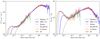 |
Fig. 1 Uncorrected source counts for the DR2 13-h field and the three LoTSS deep fields. Poissonian error bars are plotted. Left panel: conventional Euclidean scaling of the differential source counts, S5∕2 ; right panel: scaling by S2 which emphasises the contribution made by each bin to the integrated total flux density per unit area. Overplotted are the 6C source counts of Hales et al. (1988) and the functional form fitted by Intema et al. (2017) to the combined TGSS and literature source counts. |
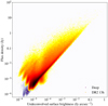 |
Fig. 2 Total flux density against a proxy of mean surface brightness for the wide and deep fields. Red/yellow colours show a density plot for the 13-h field; purples, below, show the same plot for the combination of the three deep fields described in the text. The boundary at the lower right-hand edge corresponds to unresolved sources, and at the left-hand edge to the surface brightness limit. |
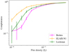 |
Fig. 3 “Flux density completeness” corrections for the three deep fields. |
3.3 Totalsky temperature
In principle the sky temperature contribution from a complete sample is easy to calculate. The spectral radiance Iν is given by
 (1)
(1)
where Si are the flux densities of individual sources in W Hz−1 m−2 and Ω is the total solid angle covered by the survey in sr. The sky brightness temperature is then given by
 (2)
(2)
Alternatively, we can integrate over the binned number counts to obtain
 (3)
(3)
where n is the differential number count, and then convert the spectral radiance to temperature in the same way.
We are in a position to make the calculation in both ways, since we can either numerically integrate the binned source counts of Fig. 4 or add up individual source flux densities applying the completeness correction to the summed fluxes. In both cases we switch between the use of the wide-field and deep-field data at a flux-density value of 4 mJy, conservatively chosen as the point where the source counts for the wide and deep surveys diverge; the actual choice of this threshold between 1 and 4 mJy makes very little difference to the results. We verify that the two possible approaches give the same answer, as expected. For all deep three fields – with the DR2 13h data supplying the bright end of the source counts – we obtain a total spectral radiance (sky surface brightness) of approximately 28 kJy sr−1 at 144 MHz. Using integration of the source counts down to the lowest levels for which we have reliable completeness corrections, we then obtain sky temperature values of 44.5 ± 3.0 K for Boötes, 43.3 ± 2.8 K for ELAIS-N1 and 45.4 ± 3.3 K for Lockman, where the error estimates take account of the flux scale uncertainties that we have assigned to the wide and deep fields (the dominant contribution) but also the statistical uncertainties on the completeness correction factor. Taking the mean of the three fields, our best estimate for the total contribution to the sky temperature of discrete sources above 100 μJy is 44.4 ± 1.7 K. We note that the effect of the flux density completeness correction is generally a boost to sky brightness or temperature by between 10 and 20%, but only of order 10% for our most reliable field, ELAIS-N1. Thus, even if our completeness corrections are over-generous as discussed above, a conservative lower limit on the contribution of discrete sources to the sky temperature would be ~ 40 K.
3.4 Consistency check using images
For the DR2 data we carried out a further consistency check to establish whether significant extended flux density was missed by the PyBDSF decomposition itself. To do this we took the mosaic images covered by our catalogue, both at high (6 arcsec) and low (20 arcsec) resolution, calculated the number of non-blank pixels and the sum of the flux density over those pixels, and so calculated a spectral radiance for each field. The mean of these values is then the mean sky brightness contributed by sources above the noise level in the wide-field data. (Because the mosaics overlap, each sky pixel is not uniformly weighted in this sum, but no bias shoud be introduced by this process.) We emphasise that it is not safe to sum over the maps alone to obtain the sky temperature, because any undeconvolved emission present will not be accounted for correctly, but the sums can be used to check whether PyBDSF is missing flux. Summing over 2.1 × 1011 pixels in the full-resolution mosaics, we obtain a mean of 21.8 ± 0.2 kJy sr−1 (statistical uncertainties only), which is in excellent agreement with the value obtained by integration of the source counts for these fields (21.8 kJy sr−1) or by direct summation of the source fluxes (21.7 kJy sr−1). Interestingly, the sum over the low-resolution mosaics is slightly higher at 22.5 ± 0.2 kJy sr−1, which could reflect either a tendency for diffuse structure to be missed in the maps and catalogues at 6 arcsec resolution or some differential calibration uncertainty between long and short baselines. The difference is only a few per cent and thus does not have a significant effect on our conclusions.
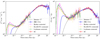 |
Fig. 4 Source counts for the deep fields with the “flux-density completeness” correction described in the text applied to the data. Lines, symbols and other source count plots as in Fig. 1. Error bars for the deep fields include the statistical uncertainties on completeness correction factors. |
4 Discussion and conclusions
We have estimated the total contribution of discrete sources between 100 μJy and 100 Jy to the sky temperatureat 144 MHz to be 44 ± 2 K. We derived this from a combination of three deep surveys, extending down to an rms noise level of 20 μJy per beam, after applying completeness corrections and deriving the bright end of the source counts from a shallower but much larger survey conducted with the same instrument and analysed using comparable techniques. Our estimate should thus include contributions from discrete sources with 144-MHz flux densities from 100 μJy to ~ 100 Jy.
Our estimate of the sky temperature from discrete sources is substantially higher than the best existing discrete source-count based estimate at these frequencies given by Vernstrom et al. (2011), who used only the 6C counts to obtain T = 18 K at 150 MHz (20 K at 144MHz)7. Our value exceeds even their highest extrapolation down to low flux densities, presumably because of the non-negligible contributionfrom both faint and diffuse sources that were not present in their extrapolation.
Our result is in remarkable agreement with the estimate of Bridle (1967) of a sky temperature for the isotropic component of 30 ± 7 K at 178 MHz (53 ± 12 K at 144 MHz) and of course is consistent with the rough upper limit on temperature from the northern-sky survey of Turtle & Baldwin (1962) (80 K at 178 MHz or 140 K at 144 MHz).
However, it is clear that the LOFAR-detected source population cannot explain the entirety of the background reported by Fixsen et al. (2011), which would correspond to 190 K at 144 MHz (we use the best-fitting power-law model from their work) and which is supported by more recent independent observations such as those of Dowell & Taylor (2018). Even with LOFAR’s sensitivity to both faint and extended sources, we are reproducing only a quarter of the ARCADE-2 background level. If the downturn in the corrected source counts below 200 μJy is to be believed (and it seems qualitatively consistent with what is expected from source count models and P(D) analysis at higher frequencies: Condon et al. 2012; Mauch et al. 2020) then no extrapolation of the currently detectable source population will make up this discrepancy; once the number counts fall below n ∝ S−2 they rapidly cease to make a significant contribution to the sky temperature. If we ignore any evidence for a downturn, then power-law extrapolation, n ∝ S−5∕2, of the observed number counts from their observed peak level at around 200 μJy down to levels of a few μJy would explain all of the ARCADE-2 background, but this is very definitely not what is expected from source models, and Condon et al. (2012) argue that such a numerous bright source population is ruled out by P(D) analysis; in any case the long baselines of LOFAR would be needed to avoid the confusion limit in studying such a source population down to the lowest flux levels.
The use of LOFAR, with its excellent sensitivity to extended emission, also rules out the possibility that a significant fraction of the excess can be due to diffuse radio emission, as discussed by, for example, Vernstrom et al. (2015), unless it is well below the sensitivity limits of even the deep surveys. The fact that we can directly account for a higher fraction of the ARCADE-2 background than has hitherto been possible may be a result of LOFAR’s excellent sensitivity to resolved sources, but if our surface brightness completeness analysis is valid then we have taken this as far as it can go. Only if a population of faint sources existed whose sizes were much larger than can be extrapolated from the > 100 mJy population (i.e., probably many arcmin in size) would we be significantly in error. Such sources would likely be modelled out in our calibration and imaging process and a dedicated low-resolution calibration and imaging of the LOFAR data might be necessary to search for them. The conclusions of Sect. 3.4 suggest that the resolution would need to be of the order of arcminutes to have any chance of revealing flux missed by the current analysis, but LOFAR surveys data tapered to arcmin resolution have significantly reduced sensitivity and so cannot be used to investigate this further.
The level of the ARCADE-2 excess is very sensitive to a model of the Galactic foreground emission; the analysis of Fixsen et al. (2011) and in particular the Galactic modelling of Kogut et al. (2011) were carried out before the most recent Planck results were available, which show a strong contribution from anomalous microwave emission (AME) in the ARCADE-2 band (Planck Collaboration XXV 2016); in addition, there is some evidence from more recent work, for example with C-BASS8 (Dickinson et al. 2019) that the spectral index of Galactic emission is steeper than the modelling of Kogut et al. (2011) would allow for. These factors might make the remaining extragalactic excess – which must exist in the data – more compatible with the levels found here and elsewhere from discrete sources.
A remaining possibility is that the ARCADE-2 excess is the result of a previously unaccounted for synchrotron background that has most of its power on such large angular scales (~ 1 degree) such that it is largely undetectable by the LOFAR observations we have used. It is hard to see how such a background could be related to a known extragalactic source population. Krause & Hardcastle (2021) will discuss a possible model in terms of emission from sources very local to the solar system (the Local Bubble).
Our findings are also relevant to the search for signals from cosmic dawn, in particular to the modelling of the foreground contributions to the sky-averaged spectrum. EDGES (Bowman et al. 2018a) reported a deficit in the extragalactic brightness temperaturedue to HI absorption of about 0.5 K at a frequency around 78 MHz. In their analysis they model ionospheric and galactic foregrounds (see also the discussion by Hills et al. 2018 and Bowman et al. 2018b), but do not address diffuse extragalactic foreground components explicitly. However, their five-parameter foreground model accounts implicitly (at least partially) for extragalactic synchrotron foregrounds as well. The steepest foreground component in their model goes as Tν ∝ν−2.5, whereas, as noted above, we would expect the extragalactic background to have a steeper spectrum. Extrapolation of our measurement at 144 MHz by means of a power-law spectrum to the frequencies probed by EDGES would imply an extragalactic brightness temperature at 78 MHz of T ≈ 235 ± 18 K, allowing for a spectral index uncertainty of ±0.1. In contrast to the Galactic and ionospheric foregrounds, the extragalactic component should be stationary and isotropic, modulated by a cosmic dipole; its magnitude would also be comparable to the claimed absorption signal. Deep fields observed with the LOFAR LBA will allow us in the future to directly probe the relevant frequency window.
Although the LOFAR deep fields used in this work represent the deepest images ever made at 100–200 MHz frequencies, it is possible to go still deeper – additional data on these fields and on others (for example, the North Celestial Pole field) exist and, on a timescale of a few years, it will be possible to improve our estimates of the contribution to the sky temperature of the < 100 μJy population.
Acknowledgments
M.J.H. would like to acknowledge conversations with Tessa Vernstrom which inspired him to make use of LOFAR data to address this science question. We are grateful to Gülay Gürkan and Alexandar Shulevksi for comments on the first draft of the paper. M.J.H. acknowledges support from the UK Science and Technology Facilities Council (ST/R000905/1). P.N.B. and J.S. are grateful for support from the UK STFC via grant ST/R000972/1. A.D. acknowledges support by the BMBF Verbundforschung under the grant 05A17STA. M.J.J. acknowledges support from the UK Science and Technology Facilities Council [ST/N000919/1] and the Oxford Hintze Centre for Astrophysical Surveys which is funded through generous support from the Hintze Family Charitable Foundation. I.P. acknowledges support from INAF under the SKA/CTA PRIN “FORECaST” and the PRIN MAIN STREAM “SAuROS” projects. LOFAR, the Low Frequency Array designed and constructed by ASTRON, has facilities in several countries, which are owned by various parties (each with their own funding sources), and are collectively operated by the International LOFAR Telescope (ILT) foundation under a joint scientific policy. The ILT resources have benefited from the following recent major funding sources: CNRS-INSU, Observatoire de Paris and Université d’Orléans, France; BMBF, MIWF-NRW, MPG, Germany; Science Foundation Ireland (SFI), Department of Business, Enterprise and Innovation (DBEI), Ireland; NWO, The Netherlands; the Science and Technology Facilities Council, UK; Ministry of Science and Higher Education, Poland. Part of this work was carried out on the Dutch national e-infrastructure with the support of the SURF Cooperative through grant e-infra 160022 & 160152. The LOFAR software and dedicated reduction packages on https:// github.com/apmechev/GRID_LRT were deployed on the e-infrastructure by the LOFAR e-infragroup, consisting of J. B. R. Oonk (ASTRON & Leiden Observatory), A. P. Mechev (Leiden Observatory) and T. Shimwell (ASTRON) with support from N. Danezi (SURFsara) and C. Schrijvers (SURFsara). This research has made use of the University of Hertfordshire high-performance computing facility (https://uhhpc.herts.ac.uk/) and the LOFAR-UK compute facility, located at the University of Hertfordshire and supported by STFC [ST/P000096/1]. The Jülich LOFAR Long Term Archive and the German LOFAR network are both coordinated and operated by the Jülich Supercomputing Centre (JSC), and computing resources on the supercomputer JUWELS at JSC were provided by the Gauss Centre for supercomputing e.V. (grant CHTB00) through the John von Neumann Institute for Computing (NIC). This research made use of ASTROPY, a community-developed core Python package for astronomy (Astropy Collaboration 2013) hosted at http://www.astropy.org/, of MATPLOTLIB (Hunter 2007), and of TOPCAT (Taylor 2005).
References
- Astropy Collaboration (Robitaille, T. P., et al.) 2013, A&A, 558, A33 [NASA ADS] [CrossRef] [EDP Sciences] [Google Scholar]
- Bowman, J. D., Rogers, A. E. E., Monsalve, R. A., Mozdzen, T. J., & Mahesh, N. 2018a, Nature, 555, 67 [NASA ADS] [CrossRef] [Google Scholar]
- Bowman, J. D., Rogers, A. E. E., Monsalve, R. A., Mozdzen, T. J., & Mahesh, N. 2018b, Nature, 564, 35 [Google Scholar]
- Bridle, A. H. 1967, MNRAS, 136, 219 [NASA ADS] [Google Scholar]
- Condon, J. J., Cotton, W. D., Fomalont, E. B., et al. 2012, ApJ, 758, 23 [NASA ADS] [CrossRef] [Google Scholar]
- Dickinson, C., Barr, A., Chiang, H. C., et al. 2019, MNRAS, 485, 2844 [Google Scholar]
- Dowell, J., & Taylor, G. B. 2018, ApJ, 858, L9 [NASA ADS] [CrossRef] [Google Scholar]
- Ewall-Wice, A., Chang, T.-C., & Lazio, T. J. W. 2020, MNRAS, 492, 6086 [Google Scholar]
- Fixsen, D. J., Kogut, A., Levin, S., et al. 2011, ApJ, 734, 5 [NASA ADS] [CrossRef] [Google Scholar]
- Hale, C. L., Williams, W., Jarvis, M. J., et al. 2019, A&A, 622, A4 [NASA ADS] [CrossRef] [EDP Sciences] [Google Scholar]
- Hales, S. E. G., Baldwin, J. E., & Warner, P. J. 1988, MNRAS, 234, 919 [Google Scholar]
- Hales, S. E. G., Masson, C. R., Warner, P. J., & Baldwin, J. E. 1990, MNRAS, 246, 256 [NASA ADS] [Google Scholar]
- Hardcastle, M. J., Gürkan, G., van Weeren, R. J., et al. 2016, MNRAS, 462, 1910 [NASA ADS] [CrossRef] [Google Scholar]
- Hardcastle, M. J., Williams, W. L., Best, P. N., et al. 2019, A&A, 622, A12 [NASA ADS] [CrossRef] [EDP Sciences] [Google Scholar]
- Heywood, I., Jarvis, M. J., & Condon, J. J. 2013, MNRAS, 432, 2625 [NASA ADS] [CrossRef] [Google Scholar]
- Hills, R., Kulkarni, G., Meerburg, P. D., & Puchwein, E. 2018, Nature, 564, E32 [CrossRef] [Google Scholar]
- Hunter, J. D. 2007, Comput. Sci. Eng., 9, 90 [NASA ADS] [CrossRef] [Google Scholar]
- Intema, H. T., Jagannathan, P., Mooley, K. P., & Frail, D. A. 2017, A&A, 598, A78 [NASA ADS] [CrossRef] [EDP Sciences] [Google Scholar]
- Kogut, A., Fixsen, D. J., Levin, S. M., et al. 2011, ApJ, 734, 4 [NASA ADS] [CrossRef] [Google Scholar]
- Kondapally, R., Best, P. N., Hardcastle, M. J., et al. 2021, A&A, 648, A3 (LoTSS SI) [EDP Sciences] [Google Scholar]
- Krause, M. G. H., & Hardcastle, M. J. 2021, MNRAS, 502, 2807 [Google Scholar]
- Mandal, S., Prandoni, I., Hardcastle, M. J., et al. 2021, A&A, 648, A5 (LoTSS SI) [EDP Sciences] [Google Scholar]
- Mauch, T., Klöckner, H.-R., Rawlings, S., et al. 2013, MNRAS, 435, 650 [NASA ADS] [CrossRef] [Google Scholar]
- Mauch, T., Cotton, W. D., Condon, J. J., et al. 2020, ApJ, 888, 61 [NASA ADS] [CrossRef] [Google Scholar]
- Mohan, N., & Rafferty, D. 2015, Astrophysics Source Code Library [record ascl:1502.007] [Google Scholar]
- Planck Collaboration XXV. 2016, A&A, 594, A25 [NASA ADS] [CrossRef] [EDP Sciences] [Google Scholar]
- Prandoni, I., Gregorini, L., Parma, P., et al. 2001, A&A, 365, 392 [NASA ADS] [CrossRef] [EDP Sciences] [Google Scholar]
- Retana-Montenegro, E., Röttgering, H. J. A., Shimwell, T. W., et al. 2018, A&A, 620, A74 [NASA ADS] [CrossRef] [EDP Sciences] [Google Scholar]
- Roger, R. S., Costain, C. H., & Bridle, A. H. 1973, AJ, 78, 1030 [NASA ADS] [CrossRef] [Google Scholar]
- Sabater, J., Best, P. N., Tasse, C., et al. 2021, A&A, 648, A2 (LoTSS SI) [EDP Sciences] [Google Scholar]
- Scaife, A. M. M., & Heald, G. H. 2012, MNRAS, 423, L30 [NASA ADS] [CrossRef] [Google Scholar]
- Shimwell, T. W., Röttgering, H. J. A., Best, P. N., et al. 2017, A&A, 598, A104 [NASA ADS] [CrossRef] [EDP Sciences] [Google Scholar]
- Shimwell, T. W., Tasse, C., Hardcastle, M. J., et al. 2019, A&A, 622, A1 [NASA ADS] [CrossRef] [EDP Sciences] [Google Scholar]
- Siewert, T. M., Hale, C., Bhardwaj, N., et al. 2020, A&A, 643, A100 [EDP Sciences] [Google Scholar]
- Singal, J., Haider, J., Ajello, M., et al. 2018, PASP, 130, 036001 [Google Scholar]
- Smirnov, O. M., & Tasse, C. 2015, MNRAS, 449, 2668 [NASA ADS] [CrossRef] [Google Scholar]
- Tasse, C. 2014, A&A, 566, A127 [NASA ADS] [CrossRef] [EDP Sciences] [Google Scholar]
- Tasse, C., Hugo, B., Mirmont, M., et al. 2018, A&A, 611, A87 [NASA ADS] [CrossRef] [EDP Sciences] [Google Scholar]
- Tasse, C., Shimwell, T., Hardcastle, M. J., et al. 2021, A&A, 648, A1 (LoTSS SI) [EDP Sciences] [Google Scholar]
- Taylor, M. B. 2005, ASP Conf. Ser., 347, 29 [Google Scholar]
- Turtle, A. J., & Baldwin, J. E. 1962, MNRAS, 124, 459 [NASA ADS] [CrossRef] [Google Scholar]
- Vernstrom, T., Scott, D., & Wall, J. V. 2011, MNRAS, 415, 3641 [NASA ADS] [CrossRef] [Google Scholar]
- Vernstrom, T., Norris, R. P., Scott, D., & Wall, J. V. 2015, MNRAS, 447, 2243 [NASA ADS] [CrossRef] [Google Scholar]
- Williams, W. L., van Weeren, R. J., Röttgering, H. J. A., et al. 2016, MNRAS, 460, 2385 [NASA ADS] [CrossRef] [Google Scholar]
ARCADE stands for “Absolute Radiometer for Cosmology, Astrophysics, and Diffuse Emission”. Although the evidence for the background discussed in this section pre-dates the ARCADE-2 result, it was the ARCADE-2 results that gave it its current prominence and so we refer to it as the ARCADE-2 background throughout the paper.
LoTSS is the LOFAR Two-Metre Sky Survey: see https://lofar-surveys.org/
Here and throughout where a temperature index is not known we convert quoted literature temperatures to 144 MHz on the assumption of a temperature index β = 2.7, T ∝ ν−β, since the spectral index of the extragalactic population is known to be α ≈ 0.7, S ∝ ν−α: see, for example, Hardcastle et al. (2016).
All Tables
All Figures
|
Fig. 1 Uncorrected source counts for the DR2 13-h field and the three LoTSS deep fields. Poissonian error bars are plotted. Left panel: conventional Euclidean scaling of the differential source counts, S5∕2 ; right panel: scaling by S2 which emphasises the contribution made by each bin to the integrated total flux density per unit area. Overplotted are the 6C source counts of Hales et al. (1988) and the functional form fitted by Intema et al. (2017) to the combined TGSS and literature source counts. |
| In the text | |
|
Fig. 2 Total flux density against a proxy of mean surface brightness for the wide and deep fields. Red/yellow colours show a density plot for the 13-h field; purples, below, show the same plot for the combination of the three deep fields described in the text. The boundary at the lower right-hand edge corresponds to unresolved sources, and at the left-hand edge to the surface brightness limit. |
| In the text | |
|
Fig. 3 “Flux density completeness” corrections for the three deep fields. |
| In the text | |
|
Fig. 4 Source counts for the deep fields with the “flux-density completeness” correction described in the text applied to the data. Lines, symbols and other source count plots as in Fig. 1. Error bars for the deep fields include the statistical uncertainties on completeness correction factors. |
| In the text | |
Current usage metrics show cumulative count of Article Views (full-text article views including HTML views, PDF and ePub downloads, according to the available data) and Abstracts Views on Vision4Press platform.
Data correspond to usage on the plateform after 2015. The current usage metrics is available 48-96 hours after online publication and is updated daily on week days.
Initial download of the metrics may take a while.