| Issue |
A&A
Volume 647, March 2021
|
|
|---|---|---|
| Article Number | A17 | |
| Number of page(s) | 14 | |
| Section | Cosmology (including clusters of galaxies) | |
| DOI | https://doi.org/10.1051/0004-6361/202038358 | |
| Published online | 01 March 2021 | |
Evolution of superclusters and supercluster cocoons in various cosmologies
1
Tartu Observatory, University of Tartu, 61602 Tõravere, Estonia
e-mail: This email address is being protected from spambots. You need JavaScript enabled to view it.
2
ICRANet, Piazza della Repubblica 10, 65122 Pescara, Italy
3
Estonian Academy of Sciences, 10130 Tallinn, Estonia
4
National Institute of Chemical Physics and Biophysics, Tallinn 10143, Estonia
Received:
6
May
2020
Accepted:
5
January
2021
Abstract
Aims. We investigate the evolution of superclusters and supercluster cocoons (basins of attraction), and the effect of cosmological parameters on the evolution.
Methods. We performed numerical simulations of the evolution of the cosmic web for different cosmological models: the Λ cold dark matter (LCDM) model with a conventional value of the dark energy (DE) density, the open model OCDM with no DE, the standard SCDM model with no DE, and the hyper-DE HCDM model with an enhanced DE density value. We find ensembles of superclusters of these models for five evolutionary stages, corresponding to the present epoch z = 0, and to redshifts z = 1, 3, 10, and 30. We used the diameters of the largest superclusters and the number of superclusters as percolation functions to describe the properties of the ensemble of superclusters in the cosmic web. We analysed the size and mass distribution of superclusters in models and in real samples based on the Sloan Digital Sky Survey.
Results. In all models, the numbers and volumes of supercluster cocoons are independent of the cosmological epochs. The supercluster masses increase with time and the geometrical sizes in comoving coordinates decrease with time for all models. The LCDM, OCDM, and HCDM models have almost similar percolation parameters. This suggests that the essential parameter, which defines the evolution of superclusters, is the matter density. The DE density affects the growth of the amplitude of density perturbations and the growth of masses of superclusters, but significantly weaker. The HCDM model has the highest speed of the growth of the density fluctuation amplitude and the largest growth of supercluster masses during the evolution. The geometrical diameters and the numbers of HCDM superclusters at high threshold densities are larger than for the LCDM and OCDM superclusters. The SCDM model has about twice as many superclusters as other models, and the SCDM superclusters have smaller diameters and lower masses.
Conclusions. We find that supercluster embryos form at very early cosmological epochs and that the evolution of superclusters occurs mainly inside their cocoons. The evolution of superclusters and their cocoons as derived from density fields agress well with the evolution found from velocity fields.
Key words: large-scale structure of Universe / dark matter / cosmology: theory / methods: numerical
© ESO 2021
1. Introduction
According to the currently accepted cosmological paradigm, the evolution of the structure of the universe started from a tiny perturbation of the primordial medium. The evolution of perturbations is affected by the physical content of the matter-energy medium and by physical processes, from inflation to matter and radiation equilibrium and beyond. The basic constituents of the matter-energy medium are dark matter (DM), dark energy (DE), and baryonic matter. For given initial density perturbations, the evolution depends on the fractional density of DM and DE, which is expressed in units of the total matter-energy density, ΩDM, and ΩΛ.
The structure of the cosmic web depends on initial density fluctuations and on various gravitational and physical processes during the evolution. Differences due to cosmological matter-energy density parameters affect the structure of the cosmic web on various scales and the time evolution of the web. The differences in the structure of the cosmic web between cold dark matter (CDM) and hot dark matter (HDM) models are well known. They affect the structure of the cosmic web on all scales. The differences in the structure of models with variable cosmological parameters in the CDM model were studied by Angulo & White (2010).
The differences in cosmological parameters affect the structure of superclusters of galaxies, which are the largest structures of the cosmic web. Until recently, superclusters were selected using the matter density field (Einasto et al. 2007; Luparello et al. 2011; Liivamägi et al. 2012). Tully et al. (2014) suggested defining superclusters on the basis of their dynamical effect on the cosmic environment, basins of attraction (BoA), as the volumes containing all points whose velocity flow lines converge on a given attractor. By this definition, BoAs mean both superclusters and their surrounding low-density regions. To keep the traditional definition of superclusters as connected high-density regions of the cosmic web, Einasto et al. (2019) proposed to call the basins of attraction “cocoons”. Superclusters are high-density regions of their cocoons.
The goal of the present paper is twofold: to investigate the evolution of superclusters and their cocoons, and to study the effect of cosmological parameters on the properties and the evolution of superclusters and their cocoons. We accept the CDM paradigm and study deviations from the standard CDM picture that are due to variations of the DM and DE content. In this approach we ignore deviations from the concordance ΛCDM model (Bahcall et al. 1999). These deviations are well known, see for example Frieman et al. (2008) and Di Valentino et al. (2020a,b, 2021). We assume that these deviations are smaller than the deviations that are due to variations in DM and DE content, and that they can be ignored in the present study. We perform numerical simulations of the evolution of the cosmic web in a box of size 1024 h−1 Mpc, using four different sets of cosmological density parameters. In three sets we use a constant DM content and vary the DE content from zero (the open OCDM model), the conventional ΛCDM model, and a model with enhanced DE content HCDM (not to be confused with hot-cold DM models, also denoted HCDM). The first of these models has an open cosmology, the second a flat cosmology, and the third a closed cosmology. The fourth model is the classical standard CDM (SCDM) model of critical density with no DE; it also has a flat cosmology. All models have identical initial phases. This facilitates determining differences between models.
We use the extended percolation analysis by Einasto et al. (2018) to describe the large-scale geometry of the cosmic web. In this method, superclusters are searched using density fields that are smoothed with an 8 h−1 Mpc kernel. We find superclusters of these models for five epochs, corresponding to the present epoch z = 0, and to redshifts z = 1, 3, 10, and 30, and compare the properties of the model superclusters with the properties of observed superclusters. We also derive the size and mass distributions of superclusters. The model size and mass distributions are compared with the size and luminosity distributions of the observed superclusters in the main galaxy survey of the Sloan Digital Sky Survey (SDSS). In calculating the density field, we used all DM particles of the simulations. The present study is a follow-up of the study by Einasto et al. (2018, 2019) of the evolution of ΛCDM superclusters, using a broader set of cosmological parameters. The evolution of supercluster BoAs was investigated by Dupuy et al. (2020) using velocity fields. This allows us to compare the evolution of superclusters and their BoAs in more detail.
The paper is organised as follows. In the next section we describe the calculation of the density fields of the simulated and observed samples and the methods we used to find superclusters and their parameters. In Sect. 3 we analyse the evolution of superclusters as described by percolation functions. In Sect. 4 we discuss the evolution of superclusters in various cosmological models and compare our results, based on the analysis of density fields, with the study of the supercluster evolution using velocity fields. The last section summarises and concludes the paper.
2. Data
To find superclusters, we determined the supercluster definition method and the basic parameters of the method. We used the density field method. We defined superclusters as the largest non-percolating high-density regions of the cosmic web, which host galaxies and clusters of galaxies, connected by filaments. Based on our experience, we used for the supercluster search the matter density field (the luminosity density field for the SDSS sample), calculated with the B3 spline with a kernel size of 8 h−1 Mpc. The determination of the second parameter of the supercluster search, the threshold density, is discussed below.
2.1. Simulation of the cosmic web
To determine the effect of cosmological parameters on the formation of superclusters, we performed four simulations with different values of the density parameters. In the concordance ΛCDM model (Bahcall et al. 1999), we accepted parameters Ωm = 0.286, ΩΛ = 0.714. In the classical standard SCDM model, we used parameters (Davis et al. 1985) Ωm = 1.000 and ΩΛ = 0. In the open OCDM model, we used Ωm = 0.286, ΩΛ = 0. In the fourth hyper-DE model HCDM, we assumed parameters Ωm = 0.286, and a higher DE density, ΩΛ = 0.914. This model is not to be confused with the hot-cold DM model, which is often denoted HCDM, but is not used in this paper. In all models we accepted the dimensionless Hubble constant h = 0.6932, and the amplitude of the linear power spectrum on the scale 8 h−1 Mpc, σ8 = 0.825. The model parameters are given in Table 1. The linear power spectra of the density perturbation at the present epoch are shown in Fig. 1.
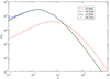 |
Fig. 1. Linear power spectra of LCDM, HCDM, OCDM, and SCDM models at the present epoch. |
Model parameters.
All models have the same realisation, so that the role of different values of the cosmological parameters can be easily compared. The initial density fluctuation spectra were generated using the COSMICS code by Bertschinger (1995). To generate the initial data, we used the baryonic matter density Ωb = 0.044 (Tegmark et al. 2004). Calculations were performed with the GADGET-2 code by Springel (2005). Particle positions and density fields were extracted for seven epochs between redshifts z = 30, …0. We selected large-scale over-density regions at five cosmological epochs, corresponding to redshifts z = 0, z = 1, z = 3, z = 10, and z = 30. The resolution of all simulations was Npart = Ncells = 5123, the size of the simulation boxes was L0 = 1024 h−1 Mpc, the volume of the simulation box was V0 = 10243 (h−1 Mpc)3, and the size of the simulation cell was 2 h−1 Mpc. This box size is sufficient to see the role of large-scale density perturbations in the evolution of the cosmic web. Using conventional terminology, we call relatively isolated high-density regions of the cosmic web clusters (Stauffer 1979). These clusters are candidates in the search for superclusters of galaxies. Superclusters have characteristic lengths of up to ≈100 h−1 Mpc (Liivamägi et al. 2012). As shown by Klypin & Prada (2019), larger simulation boxes are not needed to understand the main properties of the cosmic web. We designate the simulation with the conventional cosmological parameters LCDM.z, the standard model with high matter content SCDM.z, the model with enhanced DE content HCDM.z, and the open model as OCDM.z, where the index z shows the redshift.
2.2. SDSS data
The density field method allows us to use flux-limited galaxy samples, and to take galaxies statistically into account that are too faint to be included in the flux-limited samples, as applied for example by Einasto et al. (2003, 2007) and Liivamägi et al. (2012) to select galaxy superclusters. We used the SDSS Data Release 8 (DR8) (Aihara et al. 2011) and the galaxy group catalogue by Tempel et al. (2012) to calculate the luminosity density field. In calculating the luminosity density field, we took the selection effects in flux-limited samples into account (Tempel et al. 2009; Tago et al. 2010). In calculating the luminosity density field, we selected galaxies within the apparent r magnitude interval 12.5 ≤ mr ≤ 17.77 (Liivamägi et al. 2012). In the nearby region, relatively faint galaxies were included in the sample, but in more distant regions, only the brightest galaxies are seen. To take this into account, we calculated a distance-dependent weight factor, WL(d), following Einasto et al. (2018). The weight factor WL(d) increases to ≈8 at the far end of the sample; for a more detailed description of the calculation of the luminosity density field and the corrections we used, see Liivamägi et al. (2012). The algorithm we used to find superclusters is described below. The volume of the SDSS main galaxy sample is 5093 (h−1 Mpc)3 (Liivamägi et al. 2012).
2.3. Calculation of the density field
We calculated the smoothed density field using a B3 spline (see Martínez & Saar 2002). The B3 spline function is very similar to a Gaussian kernel, but has no extended wings. It is different from zero only in the interval x ∈ [ − 2, 2]. The B3 kernel of radius RB = 1 h−1 Mpc corresponds to a Gaussian kernel with dispersion RG = 0.6 h−1 Mpc (Tempel et al. 2014). To calculate the high-resolution density field, we used a kernel of a scale equal to the cell size of the simulation, L0/Ngrid, where L0 is the size of the simulation box, and Ngrid is the number of grid elements in one coordinate. The smoothing with index i has a smoothing radius ri = L0/Ngrid × 2i. The effective scale of the smoothing is equal to 2 × ri. The non-smoothed density field of our models with cell size 2 h−1 Mpc corresponds to a kernel RB = 2 h−1 Mpc. We applied a smoothing with a kernel of radius 8 h−1 Mpc, which corresponds to the index 2, and a Gaussian kernel RG = 4.8 h−1 Mpc.
As shown by Einasto et al. (2020a), smoothing with a B3 kernel yields density fields that are partly distorted by the insufficient resolution of our models for low-density regions and in high-density tails of the density field. This limits the application of the B3 spline methods in high- and low-density regions, but does not affect the main results of the analysis. In previous studies of superclusters, various methods were used to determine a smoothed density field: Einasto et al. (2007) and Luparello et al. (2011) used an Epanechnikov kernel to calculate density fields, and Liivamägi et al. (2012) and Einasto et al. (2019) applied B3 kernel. These studies showed that the basic properties of superclusters are almost independent of the density-smoothing method.
We calculated for each model the variance of the density contrast,
 (1)
(1)
where D(x) is the density in mean density units at location x, and summing was performed over all cells of the density field. The density field was calculated and its percolation functions were determined using the density D as argument. In the presentation of the results we apply percolation functions using as arguments the density threshold, reduced to the unit value of the standard deviation of the density contrast:
 (2)
(2)
2.4. Finding superclusters
The compilation of the supercluster catalogue consisted of several steps: calculating the density field, finding over-density regions as potential superclusters in the density field, calculating the parameters of potential superclusters, and finding the supercluster with the largest volume for a given density threshold. In this way, we chose the proper threshold density to compile the actual supercluster catalogue.
We scanned the density field in the range of threshold densities from Dt = 0.1 to Dt = 10 in mean density units. We used a linear step of densities, ΔDt = 0.1, to find over-density regions. This range covers all densities of practical interest because in low-density regions the minimum density is ≈0.1, and the density threshold to find conventional superclusters is Dt ≈ 5 (Liivamägi et al. 2012). We marked all cells with density values equal to or higher than the threshold Dt as filled regions and all cells below this threshold as empty regions.
Inside the first loop, we made another loop over all filled cells to find neighbours among filled cells. Two cells of the same type were considered as neighbours (friends) and members of the cluster when they have a common sidewall. As is traditional in the percolation analysis, over-density regions are called clusters (Stauffer 1979). Every cell can have six cells at most as neighbours. Members of clusters are selected using a friends-of-friends (FoF) algorithm: the friend of my friend is my friend. To exclude very small systems, only systems with fitness diameters of at least 20 h−1 Mpc were added to the list of over-density regions. These are clusters.
The next step was calculating the cluster parameters. We calculated the following parameters: centre coordinates xc, yc, and zc; cluster diameters (lengths) along the coordinate axes Δx, Δy, and Δz; geometrical diameters (lengths)  ; the fitness diameters (lengths) Lf discussed in the next subsection; the geometrical volumes Vg, which are defined as the volume in space where the density is equal to or greater than the threshold density Dt; and the total masses ℒ, which are the mass (luminosity) inside the density contour Dt of the cluster in units of the mean density of the sample. We also calculated the total volume of over-density regions, equal to the sum of volumes of all clusters, VC = ∑Vg, and the respective total filling factor, Ff = Nf/Ncells = VC/V0.
During the cluster search we find the cluster with the largest volume for the given threshold density. We stored in a separate file for each threshold density the number of clusters found, N, and the main data on the largest cluster: the geometrical diameter Lg, the fitness diameter Lf, the volume Vg, and the total mass (luminosity for SDSS samples) of the largest cluster. Diameters are found in h−1 Mpc, volumes in cubic h−1 Mpc, and the total masses and luminosities in units of the average cell mass and luminosity of the sample. These parameters as functions of the density threshold Dt are called percolation functions. They are needed to select the proper threshold density to compile the actual supercluster catalogue and to characterise general geometrical properties of superclusters in the cosmic web; for details of the percolation method, see Einasto et al. (2018). In total we have for every model and evolutionary stage 100 cluster catalogues (over-density regions) as potential supercluster catalogues. Each catalogue contains up to 14 thousand clusters with all cluster parameters mentioned above, depending on the model. These catalogues were used to find distributions of diameters and cluster masses.
2.5. Supercluster fitness diameters
Following Einasto et al. (2019), we defined the fitness volume of the supercluster, Vf, to be proportional to its geometrical volume, Vg, and divided by the total filling factor:
 (3)
(3)
Using the definition of the total filling factor of all over-density regions at this threshold density, Ff = VC/V0, we obtain
 (4)
(4)
The fitness volume measures the ratio of the supercluster volume to the summed volume of all superclusters (all filled over-density regions) at the particular threshold density, multiplied by the whole volume of the sample. Fitness diameters (lengths) of superclusters are calculated from their fitness volumes,
 (5)
(5)
We used the fitness diameters of the largest superclusters, Lf(Dt), as a percolation function in addition to other percolation functions such as geometrical diameters, Lg(Dt), total filling factors, Ff(Dt), and numbers of clusters, N(Dt). The fitness diameters of the largest superclusters are functions of the threshold density Dt and have a minimum at a medium threshold density. This minimum shows that the largest supercluster has the smallest volume fraction, Vg/VC. The minimum was used to find the threshold density for the supercluster selection. We considered the fitness volume of a supercluster as the volume of its basin of dynamical attraction or cocoon (Einasto et al. 2019). The sum of the fitness volumes of the supercluster cocoons is equal to the volume of the sample: ∑Vf = ∑Vg/VC × V0 = V0.
3. Evolution of superclusters as described by percolation functions
We discuss is this section the evolution of superclusters as described by percolation functions. Next we analyse the evolution of distributions of the supercluster diameters and luminosities, and the errors of the percolation parameters.
3.1. Evolution of the percolation functions of the model samples
We used the percolation functions to characterise the geometrical properties of the cosmic web and to select superclusters. Figure 2 shows geometrical length functions, Lg, the fitness diameter functions, Lf, and the numbers of clusters, N. The upper panels show these functions for the LCDM model and in the following panels for the HCDM, OCDM and SCDM models for redshifts z = 0, 1, 3, 10, and 30. An important parameter is the standard deviation (rms variance) of the density contrast, σ, which was calculated using Eq. (1) for all our models. The results are given in Table 2. In Fig. 2 we use the reduced threshold density x = (Dt − 1)/σ as the argument of the percolation functions.
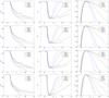 |
Fig. 2. Percolation functions of models. Left panels: geometrical length function, central panels: fitness length function, and right panels: number function. We used the reduced threshold density x = (Dt − 1)/σ as arguments of percolation functions. Diameters are given in h−1 Mpc. The panels from top to bottom show the LCDM, HCDM, OCDM, and SCDM models. |
Model parameters and SDSS superclusters.
An essential indicator of the cluster evolution is their number. Figure 2 shows the number of clusters as a function of the threshold density. At very low threshold densities, the whole over-density region contains one percolating cluster because the density field peaks are connected by filaments to a connected region. For this reason, one percolating cluster exists at a low threshold density, x ≤ 1.5 that extends over the whole volume of the computational box. The percolation threshold density, P = Dt, is defined as follows: for Dt ≤ P, one and only one percolating cluster exists, and for Dt > P, no percolating clusters exist (Stauffer 1979). We denote the percolation threshold in reduced threshold density units as xP. At these low threshold densities, the geometrical diameter of the cluster is equal to the diameter of the box,  , and its fitness diameter is equal to the side length of the box, Lf = L0.
With increasing threshold density, some filaments became fainter than the threshold density, and the connected region split into smaller units, supercluster candidates and their complexes. This led to a rapid increase in the number of clusters with increasing threshold density at x > −0.5. At x ≈ 2.6 (for the LCDM.0 model), the number of clusters reached a maximum, Nmax ≈ 8300. The threshold density at the maximum number of clusters, Dmax and xmax, the respective numbers of clusters, Nmax, and the geometrical and fitness diameters, Lg and Lf, are given in Table 2. At this threshold density, most clusters are still complexes of large over-density regions, connected by filaments to form systems with diameters of Lg ≈ 300 h−1 Mpc and Lf ≈ 200 h−1 Mpc.
When we increase x more, the number of clusters starts to decrease because the smallest clusters have maximum densities that are lower than the threshold density, and they disappear from the sample. At x ≈ 4, the geometrical and fitness diameters become equal, Lg ≈ Dd ≈ 160 h−1 Mpc. With a further increase of the density threshold geometrical diameters decrease, but the fitness diameters have a minimum and thereafter start to increase. As shown in Fig. 2 and Table 2, the minimum fitness diameters are almost identical (in co-moving coordinates) at all epochs, Lf ≈ 140 h−1 Mpc for the LCDM model. The geometrical diameter at this threshold density is Lg ≈ 115 h−1 Mpc. Both diameters are close to the conventional values of supercluster diameters. We used threshold densities at global minima of the fitness diameter functions to select supercluster ensembles. The parameters of the model supercluster samples at these threshold densities are given in Table 2. They are Dt, xt, Nscl, Lg, and Lf. The table also lists the total filling factor of over-density regions, Ff, at the threshold density Dt. This filling factor was used to find fitness volumes and diameters of superclusters, see Eq. (4). Data are given for all our model samples and evolutionary epochs.
The decrease of the number of clusters with increasing threshold continues until only the central cluster regions have densities that are higher than the threshold density. For the earliest epoch z = 30, the decrease in diameters with increasing threshold density is fastest (the diameters are expressed in co-moving coordinates).
Figure 2 and Table 2 show that the maximum numbers of clusters are very similar at all evolutionary stages of the cosmic web. This similarity, as well as the similarity of the minimum fitness diameters at different epochs, is an important property of the evolution of the cosmic web.
3.2. Diameter and mass distributions
Figure 3 shows the cumulative distributions of the geometrical and fitness diameters and supercluster masses. The data are given for all models and simulation epochs up to z = 10. Figure 3 shows that the geometrical diameters at early epochs are larger than at the present epoch (in co-moving coordinates) by a factor of approximately 2. This effect is seen in the LCDM, OCDM, and HCDM models, but it is almost absent in the SCDM model. This means that superclusters shrink during the evolution in co-moving coordinates. The fitness diameters have a different behaviour: the distribution of the fitness diameters is almost the same in co-moving coordinates at all epochs.
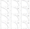 |
Fig. 3. Cumulative distribution of supercluster geometrical diameters, Lg (left panels), fitness diameters, Lf (middle panels), and total masses, ℒ (right panels). The distributions are normalised to the total supercluster numbers. Panels from top to bottom show the LCDM, HCDM, OCDM, and SCDM models. |
The right panels of Fig. 3 show that the supercluster masses increase during the evolution by a factor of approximately 3. This result agrees well with all simulations of the cosmic web growth. The skeleton of the web with supercluster embryos already forms at an early epoch. Superclusters grow by the infall of matter from low-density regions towards early forming knots and filaments, forming early superclusters. The mass growth is largest in the HCDM model.
3.3. Errors on the percolation parameters
As shown by Einasto et al. (2019), percolation parameters depend on the smoothing length that is used to calculate the density field. The changing of the smoothing length of the density field allows us to select systems of galaxies of various character, see below. For this reason, the errors of the percolation parameters characterise the accuracy of parameters in relation to galaxy systems for a given smoothing length. Some percolation functions are very smooth, and the possible parameter error is given by the step size of threshold density, which is ΔDt = 0.1 in the present study in most cases. This determines the parameter accuracy: the percolation threshold density P, the density threshold at maxima of supercluster numbers Dmax, and the density threshold for finding superclusters Dt. For early epochs the density field was scanned with a smaller step, and the possible errors on these parameters are lower. The errors on other parameters depend on the speed of the parameter changes as functions of the density threshold. The possible error range can be estimated from the parameter spread for different models and evolution epochs in Figs. 6 and 7.
4. Discussion
We start with the comparison of model percolation functions with percolation functions of observed SDSS samples. Next we discuss the evolution of the ensemble of superclusters in models with different cosmological parameters. Then we compare the evolution of LCDM and SCDM models, and evolution of LCDM, OCSM, and HCDM models. Thereafter we discuss the influence of smoothing length to properties of selected systems, and the concept of cocoons of the cosmic web. Finally we compare our analysis with results of the study of the velocity field to detect supercluster cocoons.
4.1. Comparison with SDSS samples
In Fig. 4 we compare percolation functions of observed SDSS samples with the percolation functions of the models at the present epoch. We note that there are approximately eight times more model superclusters than SDSS superclusters. This difference is due to the larger size of our model samples, 1024 h−1 Mpc, which is about twice the effective size of the SDSS main galaxy sample, 509 h−1 Mpc. To bring percolation functions of SDSS samples to the same scale as that model functions, the threshold densities of the SDSS samples must be shifted. A similar shift in the density threshold of the SDSS samples was made by Einasto et al. (2019). The densities are expressed in mean density units. In the model samples, the mean density includes DM in low-density regions in addition to the clustered matter with simulated galaxies. Low-density regions include no simulated galaxies, or the galaxies are fainter than the magnitude limit of the observational SDSS survey. For this reason, unclustered and low-density DM is not included in calculations of the mean density of the observed SDSS sample. This means that in the calculation of densities in mean density units, the densities are divided into a smaller number, which increases the density values of the SDSS samples. Einasto et al. (2019) estimated this correction factor by a trial-and-error procedure and calculated corrected threshold densities by dividing the threshold densities of the SDSS samples by the factor b = Dt/(Dt)c. We applied the same factor b = 1.30 and used it to calculate SDSS percolation functions for comparison. The corrected SDSS supercluster diameter, filling factor, and number functions agree well with the LCDM model functions.
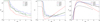 |
Fig. 4. Comparison of the percolation functions of models with SDSS samples. The model functions are plotted with coloured bold lines. The functions for SDSS samples are plotted with dashed black lines for the density correction factor 1.30. Left panel: geometrical length functions, middle panel: fitness length functions, and right panel: number functions. |
Figure 5 shows the cumulative distributions of the diameters and masses of the model samples at the present epoch and the respective distributions for the SDSS samples. To calculate the luminosity distribution of the SDSS superclusters, we divided the supercluster luminosities into the normalising factor b = 1.45, following Einasto et al. (2019). The right panel in Fig. 5 shows that this correction brings the total luminosity distributions of the SDSS and LCDM samples to a very good agreement. The diameter and luminosity distributions are shown in Figs. 3 and 5. The distributions of the different models clearly have an approximately similar character.
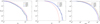 |
Fig. 5. Comparison of the cumulative diameter and mass (luminosities) distribution of models at the present epoch and the SDSS samples. Left panel: cumulative distributions of supercluster geometrical diameters Lg, middle panel: distributions of the fitness diameters Lf, and right panel: total mass (luminosity) distributions ℒ, given in units of the mass (luminosity) of one cell. The SDSS distributions are given for a threshold density Dt = 5.4, and the distribution of SDSS total luminosities is calculated for a correction factor b = 1.45. |
4.2. Evolution of the percolation parameters of supercluster ensembles
We showed in Fig. 2 that the basic characteristics of the evolution of the percolation functions in different cosmologies are rather similar. At the earliest epoch z = 30, the percolation functions, expressed as functions of the reduced threshold densities x, are almost identical for models with different cosmological parameters. The maxima of the number functions and the minima of the fitness length functions are located in all models at the earliest epoch z = 30 at a reduced threshold density xmax = 2.4. At the present epoch z = 0, the maximum shifts to xmax = 2.6 for all models. The shape of the fitness length and the number functions at early epoch is approximately symmetrical around x = xmax when expressed as a function of the reduced threshold density x. It is surprising that in spite of different values of σ at the earliest epoch z = 30, the percolation functions of all models at early epoch are so similar. At later epochs, this symmetry of the percolation functions is better preserved in the LCDM, HCDM, and OCDM models. The evolution of the SCDM model is different: at later epochs, the percolation functions of the SCDM model are shifted far more strongly to higher threshold densities than in other models, see Figs. 4 and 5.
Now we discuss the evolution of the percolation parameters of the ensemble of superclusters in more detail. In Fig. 6 we show the change in three percolation parameters of supercluster ensembles with cosmic epoch z: the filling factor Ff, the minimal fitness lengths Lf, and the maximum number of superclusters Nmax. The left panel of Fig. 6 shows the change in the filling factor Ff of the models during the evolution. This filling factor was used to calculate the fitness volumes of superclusters Vf using Eq. (3). At the earliest epoch z = 30, the filling factor of the superclusters in all models was Ff ≈ 0.02. During the evolution, the filling factor decreased in the LCDM, HCDM, and OCDM models to Ff ≈ 0.007, but it remained almost the same Ff ≈ 0.02 for the SCDM model.
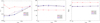 |
Fig. 6. Evolution of percolation parameters of supercluster ensembles. Left panel: change in filling factor Ff in the models with cosmic epoch z. Middle panel: evolution of the minimum fitness lengths with epoch Lf(z). Right panel: evolution of the maximum numbers of clusters with epoch N(z). |
In the middle and right panels of Fig. 6 we show the minimum fitness diameters and maximum numbers of superclusters as functions of the cosmic epoch. The LCDM, HCDM, and OCDM models have almost identical evolutions of the sizes and supercluster numbers. The maximum length of the fitness diameter of the SCDM model is about 100 h−1 Mpc, which is a factor of about 1.5 times smaller than in other models, Lf ≈ 140 h−1 Mpc. The maximum number of SCDM superclusters is almost twice as high as the number in other models. The difference of the SCDM model from other models in the maximum number of superclusters and in the minimum fitness length of SCDM superclusters is an essential finding of the present paper. We conclude that the structure of the ensemble of SCDM superclusters differs considerably from the structure of the ensemble of superclusters in other models.
Figure 7 shows the evolution of three parameters of the ensembles of models: the reduced percolation threshold xP, the reduced density threshold at the maxima of the numbers of superclusters xmax, and the reduced density threshold for finding superclusters xt. The reduced percolation lengths of the LCDM models of different box sizes and smoothing scales have mean values xP = 1.5 ± 0.1 for all simulation epochs (Einasto et al. 2019). Our study shows that models with different cosmology also have a reduced percolation length xP ≈ 1.5 for the LCDM, HCDM, and OCDM models for all cosmic epochs, which confirms early results by Colombi et al. (2000). The SCDM model has the value xP = 1.5 only for the earliest epoch z = 30. At later epochs, the reduced percolation threshold is lower, see the left panel of Fig. 7.
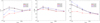 |
Fig. 7. Evolution of reduced percolation parameters of supercluster ensembles. Left panel: evolution of the reduced percolation threshold with cosmic epoch. Middle panel: change in evolution of the reduced density threshold at the maxima of the numbers of superclusters. Right panel: evolution of the reduced density threshold for finding superclusters. |
The reduced density threshold at the maxima of the number of superclusters is xmax = 2.4 for all models at the earliest epoch z = 30. During the evolution, the reduced density threshold at the maxima of the number of superclusters increases to xmax = 2.6 for all models. The reduced threshold density at the minimum of the fitness length (optimal to select superclusters) is at the earliest epoch xt = 2.6 for all models. It increases to a value xt = 5.0 for the LCDM and OCDM models, and to xt = 5.7 for the HCDM model, but it remains almost the same, xt = 3.2, for the SCDM model.
Einasto et al. (2019) investigated the evolution of the standard deviation in ΛCDM (LCDM) models of various box lengths and different smoothing scales. The authors showed that the shape of the relation between the density contrast σ and redshift 1 + z is approximately linear when expressed in log-log format. The slope of the relation is the same for the LCDM models of different box lengths and smoothing scales, and the amplitude depends on the smoothing scale. In the present paper we used identical box sizes and smoothing scales, but varied the cosmological model parameters. The variance of the standard deviation σ as a function of the cosmic epoch z is shown in the left panel of Fig. 8. The relation between σ and 1 + z is almost linear when expressed in log-log format, which agrees well with linear perturbation theory; see the right panel of Fig. 8. The HCDM model has a more rapid increase of the standard deviation σ with time (decreasing z), and the OCDM model has the slowest increase of the standard deviation with time.
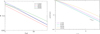 |
Fig. 8. Evolution of the standard deviation (dispersion) of density fluctuations. Left panel: change in dispersion of the density fluctuations σ with cosmic epoch z for our models. Right panel: evolution of the dispersion of the density fluctuations σ with cosmic epoch z according to the linear evolution model, normalised to the present epoch. |
4.3. Comparison of the evolution of the LCDM and SCDM models
Our analysis has shown that the properties of the SCDM model deviate strongly from the properties of other models. The main reason for this difference lies in the power spectrum of the SCDM model: it has much more power on small scales and less power on large scales. The evolution of the ensemble of superclusters in our SCDM and LCDM models can be followed in Fig. 9. The upper and middle panels of this figure show cross sections of the density fields of the LCDM model and the lower panels show the SCDM model. The panels from left to right correspond to density fields at epochs z = 30, 10, 3, and 0, calculated with co-moving smoothing kernel with a radius 8 h−1 Mpc. The models were calculated with identical phases of the initial density fluctuations. For this reason, the small-scale features of the density fields of the different models are rather similar. However, large-scale features on supercluster scales are different. In the SCDM model structures are smaller in size. To see better details we plot in Fig. 9 only central 341 × 341 h−1 Mpc sections of density fields.
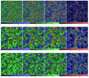 |
Fig. 9. Evolution of the density fields of LCDM and SCDM models. Upper panels: density fields of the LCDM model found with a smoothing kernel of radius 2 h−1 Mpc. Middle and lower panels: density fields of the LCDM and SCDM models found with a smoothing kernel with a radius 8 h−1 Mpc. The panels from left to right correspond to epochs z = 30, 10, 3, and 0. Cross sections are shown in a 2 h−1 Mpc thick layer of size 341 × 341 h−1 Mpc. Densities are expressed on a linear scale. Colour scales from left to right in the upper panel are 0.8−1.2, 0.6−1.45, 0.3−2, and 0.1−5.0, and in the middle and lower panels, they are 0.9−1.1, 0.8−1.25, 0.4−1.65, and 0.2−3.0. |
The left panels of Fig. 9 show the density fields of the models for a very early epoch, corresponding to redshift z = 30. The comparison of the panels of both models at identical epochs suggests that the principal large-scale structural elements of the cosmic web were present at all epochs considered here. There are differences on small scales, but the main large-scale elements of the web are seen at similar locations at all epochs. The basic visible changes are the increase in density contrast: the density distributions at epochs z = 30, z = 10, and z = 3 are very similar, only the amplitude of density perturbations has increased. In this redshift range the evolution is mainly linear, only the density contrast has increased. In later epochs the non-linear evolution is dominant, as seen by comparison of fields at z = 3 and z = 0. In the SCDM model the superclusters are smaller and their spatial density is higher than in the LCDM model.
4.4. Comparison of the evolution of the LCDM, OCDM, and HCDM models
The differences in the evolution of the cosmic web are related to the differences in their initial power spectra. Figure 1 shows that the spectra of the LCDM, OCDM, and HCDM models are identical on medium and small scales. On the largest scales the open OCDM model has a larger power than the conventional LCDM model and the hyper-DE HCDM model has a lower power. Because differences in power spectra are very small, we expect to observe also small differences in the geometrical properties of the cosmic web, as represented in these models. The DE contribution to the matter and energy density in early epochs was very small, which may explain the low sensitivity of the cosmic web properties to the DE density. The HCDM model has the highest speed of the growth of the amplitude of density fluctuations, σ, which may explains the largest growth of the supercluster masses during the evolution, as shown in Fig. 3. For the same reason, the geometrical diameters and numbers of HCDM superclusters at high threshold densities are larger than for the LCDM and OCDM superclusters.
4.5. Superclusters as great attractors in the cosmic web
All massive bodies are gravitational attractors. Galaxy-type and larger attractors are of interest in cosmology. It is well known that smoothing affects the character of the high-density regions that are found. Smoothing with a kernel of length 1 h−1 Mpc highlights ordinary galaxies together with their satellite systems, similar to our Galaxy and M 31. These attractors can be called small in the cosmological context. Within their spheres of dynamical influence, galaxy-type attractors are surrounded by dwarf satellites and intergalactic matter inside their DM halos. The central galaxies of these systems grow by infall of gas and merging of dwarf galaxies; for a detailed overview, see Wechsler & Tinker (2018). Einasto et al. (1974a) called these systems hypergalaxies. The authors suggested that hypergalaxies are primary sites of galaxy formation, and that galaxies do not form in isolation because dwarf galaxies primarily exist as satellites of brighter (central) galaxies. The radius of satellite systems and of the DM halo that surrounds the system, that is, hypergalaxies, is about 1 h−1 Mpc. For early evidence, see Einasto et al. (1974b,c).
Smoothing with a kernel of length 4 h−1 Mpc finds high-density regions of the cosmic web that have an intermediate character between clusters and traditional superclusters, such as central regions of superclusters (Einasto et al. 2012, 2020b). As shown by Einasto et al. (2019), smoothing with a 4 h−1 Mpc kernel finds four times more isolated high-density systems than smoothing with an 8 h−1 Mpc length using the same LCDM model. When a larger smoothing length of 16 h−1 Mpc is used for this model, four times fewer supercluster-type systems are found, and superclusters are larger than superclusters found with the 8 h−1 Mpc kernel.
Long experience in the study of superclusters on the basis of density fields has shown that the optimal smoothing length for finding superclusters is 8 h−1 Mpc; see Einasto et al. (2007), Luparello et al. (2011), and Liivamägi et al. (2012). Superclusters are great attractors. Supercluster centres lie at the centres of deep potential wells. They collect material from a much larger region than clusters. The slope of the potential field determines the speed of particles at a given location. Thus superclusters at different levels of the potential field have different strength as attractors.
4.6. Comparison with superclusters found from velocity data
The property of superclusters to act as great attractors was the basis of the suggestion of Tully et al. (2014), Pomarède et al. (2015), and Graziani et al. (2019) that superclusters should be defined on the basis of their dynamical effect on the cosmic environment, the so-called basins of attraction (BoA). To keep the term “superclusters” in its conventional meaning, Einasto et al. (2019) suggested to use the term “cocoons” for Tully’s BoAs. Neighbouring cocoons have common sidewalls. Einasto et al. (2019) suggested that a good measure for estimating the size of cocoons is the fitness diameter, which remains almost constant during the cosmic evolution in co-moving coordinates. According to the definition of the cocoon sizes through the fitness diameter, cocoons fill the whole volume of the observable universe, see Eq. (4).
Dupuy et al. (2019) applied constrained simulations in a ΛCDM model of length 500 h−1 Mpc, based on data from Cosmicflows-2 (Tully et al. 2013) and Cosmicflows-3 (Tully et al. 2016), and identified several BoAs. The BoA diameters calculated from volumes D = V1/3 are 79, 89, and 100 h−1 Mpc for the Laniakeia, Perseus-Pisces, and Coma supercluster BoAs, respectively. According to our analysis, the SDSS sample has 844 superclusters. The fitness diameter of the largest SDSS supercluster cocoon is 132 h−1 Mpc, the median fitness diameter of the cocoons is 41 h−1 Mpc, and the fitness diameters of 10% of largest cocoons are larger than or equal to 84 h−1 Mpc. The methods for defining the sizes of BoAs and our cocoons are different (velocity and density fields, respectively), but the numerical results for the sizes are similar.
Dupuy et al. (2020) used the SmallMultiDark simulations by Klypin et al. (2016) to segment the universe into dynamically coherent basins applying various smoothing lengths to velocity data. This simulation was performed in a box of size 400 h−1 Mpc, using 38403 particles. The density and velocity fields were calculated in a 2563 grid. The evolution of basins was followed in redshift intervals from z = 2.89 to z = 0. To test the effect of smoothing, the final velocity field was Gaussian smoothed with dispersions rs = 1.5 to 15 h−1 Mpc. Basins were searched for using three parameters: the smoothing length, the maximum streamlines length, and the integration step along streamlines. At optimal search parameters, the number of basins converged to 647 for a smoothing scale 1.5 h−1 Mpc, to about 250 basins for a smoothing scale 3 h−1 Mpc, and to only a few for smoothing scale 15 h−1 Mpc. Taking the size of the simulation box into account, these numbers agree fairly well with the number of SDSS superclusters and with the respective number in our present LCDM model. As in our LCDM model, the number of the Dupuy et al. (2020) basins decreases slightly with cosmic epoch from about 760 at z = 2.89 to 647 at z = 0. The mass distribution of the basins is almost independent of the redshifts, see Figs. 9 and 10 of Dupuy et al. (2020).
It is interesting to compare the evolution of supercluster cocoons and superclusters. We show in Fig. 10 the distribution of supercluster masses in our LCDM model at various epochs. The left panel of Fig. 10 shows the distribution of supercluster masses, and the right panel shows the cumulative distribution of supercluster masses, normalised to the total number of superclusters. For comparison we also show the cumulative distribution of supercluster masses for an LCDM model of size L0 = 512 h−1 Mpc by Einasto et al. (2019). The comparison of the evolution of superclusters and cocoons shows that the number of superclusters as well cocoons remains almost constant during the evolution. The differences in the evolution are more interesting, however. The cocoon masses remain constant during the evolution (Dupuy et al. 2020), whereas the supercluster masses increase during the evolution by a factor of about 3, see the right panel of Fig. 10.
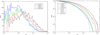 |
Fig. 10. Evolution of supercluster masses of LCDM models. Left: distribution of supercluster masses of the LCDM model at various epochs. Right: cumulative distributions of supercluster masses of the LCDM models. For comparison we show the cumulative supercluster mass distribution for a ΛCDM model with side length L0 = 512 h−1 Mpc. Masses are given in solar units. |
The second important difference is in masses themselves. Figure 10 shows that the most massive LCDM superclusters have masses M ≈ 1016 M⊙ at the present epoch. Figure 9 of Dupuy et al. (2020) shows that most massive supercluster basins (cocoons) have masses M ≈ 2 × 10¹⁷ M⊙ at all epochs. This difference is expected. The supercluster volumes at the early epoch are about 50 times smaller than the supercluster cocoon volumes; at the present epoch, this difference has increased to about 140 times, see Eq. (4), Table 2, and Fig. 8. The difference of masses of superclusters and cocoons at the present epoch is only a factor of about 20. This means that cocoon regions outside superclusters have much lower densities than inside superclusters. Because the cocoon masses remain constant during the evolution, the growth of supercluster masses can be explained by the infall of surrounding matter inside cocoons to superclusters. To illustrate the growth of superclusters, we show in the upper and middle panels of Fig. 9 the LCDM model density fields at redshifts z = 30, 10, 3, and 0 at two smoothing scales, 2 h−1 Mpc and 8 h−1 Mpc. The supercluster contraction can be followed in the upper panels, most strongly at redshift z < 1. See also Fig. 10 for the increase in supercluster masses at z < 1. The exchange of matter between cocoons is minimum because the velocity flow within the cocoons is directed inwards.
Figure 10 shows that the mass distribution of superclusters in models of size 512 and 1024 h−1 Mpc is approximately similar. However, the model of size 1024 h−1 Mpc contains slightly more massive superclusters at all simulation epochs. This small difference can be explained by the larger volume of the 1024 h−1 Mpc model: there are 6044 superclusters in the 1024 h−1 Mpc model versus 995 superclusters in the L512 model.
4.7. Evolution of superclusters and supercluster cocoons
Available data suggest that galaxy and supercluster embryos were created by high peaks in the initial field. The initial velocity field around peaks is almost laminar. The development of the density field in the early phase is well described by the Zeldovich (1970) approximation (ZA) and its extension, the adhesion model by Kofman & Shandarin (1988). As shown by Kofman et al. (1990, 1992), the adhesion approximation yields structures that are very similar to structures calculated with N-body numerical simulations of the cosmic web evolution with the same initial fluctuations. Bernardeau & Kofman (1995) compared the evolution of density fields by ZA with the results obtained by various other approximations, and found that various methods agreed well.
In the modern simulations of the cosmic web evolution we applied here, the early evolution was calculated using ZA. The structure at the first epoch used in our study, corresponding to redshift z = 30, is obtained by ZA. Figure 9 shows that the density distributions at epochs z = 30 and z = 10 are very similar, only the fluctuation amplitude has increased. Large-scale supercluster-type structures are clearly visible at all epochs, and the growth of superclusters inside cocoons is well visible. On supercluster scales the results obtained for different epochs and simulation cube sizes agree very well; see Einasto et al. (2020a).
Pichon et al. (2011) and Dubois et al. (2012, 2014) showed that a significant fraction of the cold gas falls along filaments that are oriented nearly radially to the centres of high-redshift rare massive haloes. This process rapidly increases the mass of the central halo. We may conclude that depending on the height of the initial density peak, galaxy embryos, galaxy clusters, and superclusters were created in this way. However, the further evolution of superclusters differs from the evolution of galaxies and galaxy clusters. Galaxies and ordinary galaxy clusters are local attractors and collect additional matter from their local environment. Supercluster are global attractors and collect matter from a much larger environment.
The density field method applied in this paper allows us to select superclusters of the cosmic web and to estimate the size of their cocoons. As discussed above, at the early epoch, superclusters are approximately 50 times smaller than their cocoons, and at the present epoch, they are about 140 times smaller. Our density field method allows us to select individual superclusters and to find statistical properties of the ensemble of cocoons. The velocity field method allows us to find individual supercluster cocoons, but not superclusters themselves. Thus these methods are complementary.
The filamentary character of the cosmic web can be described using the skeleton, that is, the 3D analogue of ridges in a mountainous landscape (Pichon et al. 2010). Peaks of the cosmic web are connected by filaments. The number of filaments that connect the clusters with other clusters can be called the connectivity for global connections (including bifurcation points), and multiplicity for local connections (Codis et al. 2018). Kraljic et al. (2020) investigated the connectivity of the SDSS galaxy sample. The authors first determined the skeleton of the SDSS sample, traced by the DisPerSE algorithm by Sousbie (2011). Then they calculated the connectivity of all clusters. They found that the connectivity of the SDSS sample clusters has a peak at 3, and the multiplicity (local connectivity) has a peak at 2. Both parameters depend on the cluster mass. The mean connectivity of massive SDSS clusters is 4, and the multiplicity of most massive clusters is 6.
These results have a simple explanation. Low- and medium-mass clusters lie inside filaments, and thus have the multiplicity 2 (the connection is from both sides of the cluster inside the filament). Clusters move together with filaments in the large potential well of superclusters. The simultaneous movement of clusters with their surrounding filament follows from the simple fact that the filamentary character of the cosmic web is preserved at the present epoch. If clusters had high peculiar velocities with respect to the surrounding filaments, the filamentary character of the web would be destroyed during the evolution. The laminar character of the velocity field is explained by the presence of the DE, as suggested already by Sandage et al. (2010). Very rich clusters are central clusters of superclusters, and they are connected with other structures by many filaments. This has been demonstrated by Tully & Fisher (1978) for the Virgo supercluster, by Jõeveer & Einasto (1977, 1978) and Jõeveer et al. (1978) for the Perseus-Pisces supercluster, and by Einasto et al. (2020b) for the A2142 supercluster. The central clusters of these superclusters lie at minima of potential wells created by respective superclusters. They are fed by filaments from several sides, and are suitable locations for cluster merging, which means that small clusters fall onto the central cluster along filaments surrounding the central cluster. The pattern of the cosmic web suggests that the high connectivity can be used as a signature for the presence of a central cluster of a supercluster.
5. Summary remarks
We calculated the percolation functions of superclusters for four evolutionary epochs of the Universe, corresponding to redshifts z = 30, 10, 3, 1, and z = 0. The analysis was made for four sets of cosmological models: the LCDM model, the classical standard SCDM model, the open OCDM model, and the hyper-DE HCDM model. Ensembles of superclusters were found for these four models for all evolutionary epochs. All models have the same initial phase realisation, so that we can follow the role of different values of cosmological parameters in the evolution of superclusters and their cocoons.
The almost constant number of superclusters and of the (co-moving) volume of cocoons during the evolution means that supercluster embryos were created at a very early evolution epoch, much earlier than epochs tested in this study, z = 30. On the other hand, the differences in numbers and volumes between different cosmological models at all epochs suggest that these differences were also created at an early epoch, most likely after the end of inflation and before matter and radiation equilibrium. The differences between models suggest that the supercluster and supercluster cocoon properties as measured by the percolation method using the density field and by the velocity field as done by Dupuy et al. (2020) can be used to test the basic cosmological model parameters.
We analysed the evolution of superclusters and their cocoons by applying percolation functions of the density field. Dupuy et al. (2020) studied the evolution of supercluster basins of attraction using the velocity field. Both methods yield an approximately equal spatial density of supercluster cocoons with rather similar properties. This similarity suggests that the density as well the velocity fields can be used to detect superclusters and their cocoons and to investigate their properties and evolution. The velocity field is physically more justified when velocity data are available. It can only be used today to study the nearby space of the real universe, however. For more distant regions the density field method is the only option, at least at the moment. The velocity-field-based method allows us to separate individual supercluster cocoons, and the density field method allows us to separate individual superclusters.
A more detailed study of the differences in the evolution of the LCDM, OCDM, and HCDM models is beyond the scope of the present paper. The basic conclusions of our study are listed below.
-
The combined analysis of the density and velocity field evolution shows that superclusters and their cocoons evolve differently.
-
Volumes (in comoving coordinates), masses, and numbers of supercluster cocoons are stable parameters and are almost identical for all evolutionary epochs. This suggests that embryos of supercluster cocoons were created at an early epoch. At epoch z = 30, superclusters have volumes about 50 times lower than their cocoons. At the present epoch, supercluster volumes are about 140 times lower than the volumes of their cocoons. Supercluster masses are about 20 times lower than the cocoon masses. Supercluster masses increase by about a factor of 3 during the evolution, and their volumes (in co-moving coordinates) decrease by about the same factor. Superclusters mainly evolve inside their cocoons.
-
The LCDM, OCDM, and HCDM models have almost similar percolation parameters. This suggests that the essential parameter that defines the supercluster evolution is the matter density. The DE density affects the growth of the density perturbation amplitude and the growth of supercluster masses, albeit significantly weaker. The HCDM model has the highest growth speed of the density fluctuation amplitude and the largest growth of supercluster masses during the evolution. The geometrical diameters and numbers of HCDM superclusters at high threshold densities are larger than for LCDM and OCDM superclusters. The SCDM model has about twice more superclusters than the other models. The SCDM superclusters are smaller, and their mass is lower than in other models.
Acknowledgments
Authors thank the anonymous referee for useful suggestions. This work was supported by institutional research funding IUT40-2 of the Estonian Ministry of Education and Research, by the Estonian Research Council grant PRG803, and by Mobilitas Plus grant MOBTT5. We acknowledge the support by the Centre of Excellence “Dark side of the Universe” (TK133) financed by the European Union through the European Regional Development Fund. We thank the SDSS Team for the publicly available data releases. Funding for the SDSS and SDSS-II has been provided by the Alfred P. Sloan Foundation, the Participating Institutions, the National Science Foundation, the US Department of Energy, the National Aeronautics and Space Administration, the Japanese Monbukagakusho, the Max Planck Society, and the Higher Education Funding Council for England. The SDSS website is http://www.sdss.org/. The SDSS is managed by the Astrophysical Research Consortium for the Participating Institutions. The Participating Institutions are the American Museum of Natural History, Astrophysical Institute Potsdam, University of Basel, University of Cambridge, Case Western Reserve University, University of Chicago, Drexel University, Fermilab, the Institute for Advanced Study, the Japan Participation Group, Johns Hopkins University, the Joint Institute for Nuclear Astrophysics, the Kavli Institute for Particle Astrophysics and Cosmology, the Korean Scientist Group, the Chinese Academy of Sciences (LAMOST), Los Alamos National Laboratory, the Max-Planck-Institute for Astronomy (MPIA), the Max-Planck-Institute for Astrophysics (MPA), New Mexico State University, Ohio State University, University of Pittsburgh, University of Portsmouth, Princeton University, the United States Naval Observatory, and the University of Washington.
References
- Aihara, H., Allende Prieto, C., An, D., et al. 2011, ApJS, 193, 29 [NASA ADS] [CrossRef] [Google Scholar]
- Angulo, R. E., & White, S. D. M. 2010, MNRAS, 405, 143 [NASA ADS] [Google Scholar]
- Bahcall, N. A., Ostriker, J. P., Perlmutter, S., & Steinhardt, P. J. 1999, Science, 284, 1481 [NASA ADS] [CrossRef] [Google Scholar]
- Bernardeau, F., & Kofman, L. 1995, ApJ, 443, 479 [NASA ADS] [CrossRef] [Google Scholar]
- Bertschinger, E. 1995, ArXiv e-prints [arXiv:astro-ph/9506070] [Google Scholar]
- Codis, S., Pogosyan, D., & Pichon, C. 2018, MNRAS, 479, 973 [NASA ADS] [CrossRef] [Google Scholar]
- Colombi, S., Pogosyan, D., & Souradeep, T. 2000, Phys. Rev. Lett., 85, 5515 [NASA ADS] [CrossRef] [Google Scholar]
- Davis, M., Efstathiou, G., Frenk, C. S., & White, S. D. M. 1985, ApJ, 292, 371 [NASA ADS] [CrossRef] [Google Scholar]
- Di Valentino, E., Melchiorri, A., & Silk, J. 2021, ApJ, 908, L9 [CrossRef] [Google Scholar]
- Di Valentino, E., Melchiorri, A., Mena, O., & Vagnozzi, S. 2020a, Phys. Rev. D, 101, 063502 [Google Scholar]
- Di Valentino, E., Melchiorri, A., & Silk, J. 2020b, Nat. Astron., 4, 196 [CrossRef] [Google Scholar]
- Dubois, Y., Pichon, C., Haehnelt, M., et al. 2012, MNRAS, 423, 3616 [NASA ADS] [CrossRef] [Google Scholar]
- Dubois, Y., Pichon, C., Welker, C., et al. 2014, MNRAS, 444, 1453 [NASA ADS] [CrossRef] [Google Scholar]
- Dupuy, A., Courtois, H. M., Dupont, F., et al. 2019, MNRAS, 489, L1 [NASA ADS] [CrossRef] [Google Scholar]
- Dupuy, A., Courtois, H. M., Libeskind, N. I., & Guinet, D. 2020, MNRAS, 493, 3513 [CrossRef] [Google Scholar]
- Einasto, J., Jaaniste, J., Jôeveer, M., et al. 1974a, Tartu Astr. Obs. Teated, 48, 3 [Google Scholar]
- Einasto, J., Kaasik, A., & Saar, E. 1974b, Nature, 250, 309 [NASA ADS] [CrossRef] [Google Scholar]
- Einasto, J., Saar, E., Kaasik, A., & Chernin, A. D. 1974c, Nature, 252, 111 [NASA ADS] [CrossRef] [Google Scholar]
- Einasto, J., Einasto, M., Hütsi, G., et al. 2003, A&A, 410, 425 [NASA ADS] [CrossRef] [EDP Sciences] [Google Scholar]
- Einasto, J., Einasto, M., Tago, E., et al. 2007, A&A, 462, 811 [NASA ADS] [CrossRef] [EDP Sciences] [Google Scholar]
- Einasto, M., Liivamägi, L. J., Tempel, E., et al. 2012, A&A, 542, A36 [NASA ADS] [CrossRef] [EDP Sciences] [Google Scholar]
- Einasto, J., Suhhonenko, I., Liivamägi, L. J., & Einasto, M. 2018, A&A, 616, A141 [NASA ADS] [CrossRef] [EDP Sciences] [Google Scholar]
- Einasto, J., Suhhonenko, I., Liivamägi, L. J., & Einasto, M. 2019, A&A, 623, A97 [NASA ADS] [CrossRef] [EDP Sciences] [Google Scholar]
- Einasto, J., Hütsi, G., Liivamägi, L. J., & Einasto, M. 2020a, A&A, submitted [arXiv:2011.13292] [Google Scholar]
- Einasto, M., Deshev, B., Tenjes, P., et al. 2020b, A&A, 641, A172 [CrossRef] [EDP Sciences] [Google Scholar]
- Frieman, J. A., Turner, M. S., & Huterer, D. 2008, ARA&A, 46, 385 [NASA ADS] [CrossRef] [Google Scholar]
- Graziani, R., Courtois, H. M., Lavaux, G., et al. 2019, MNRAS, 488, 5438 [CrossRef] [Google Scholar]
- Jõeveer, M., & Einasto, J. 1977, Estonian Academy of Sciences Preprint, 3 [Google Scholar]
- Jõeveer, M., & Einasto, J. 1978, in Large Scale Structures in the Universe, eds. M. S. Longair, & J. Einasto, IAU Symp., 79, 241 [Google Scholar]
- Jõeveer, M., Einasto, J., & Tago, E. 1978, MNRAS, 185, 357 [NASA ADS] [CrossRef] [Google Scholar]
- Klypin, A., & Prada, F. 2019, MNRAS, 489, 1684 [CrossRef] [Google Scholar]
- Klypin, A., Yepes, G., Gottlöber, S., Prada, F., & Heß, S. 2016, MNRAS, 457, 4340 [NASA ADS] [CrossRef] [Google Scholar]
- Kofman, L. A., & Shandarin, S. F. 1988, Nature, 334, 129 [NASA ADS] [CrossRef] [Google Scholar]
- Kofman, L., Pogosian, D., & Shandarin, S. 1990, MNRAS, 242, 200 [NASA ADS] [CrossRef] [Google Scholar]
- Kofman, L., Pogosyan, D., Shandarin, S. F., & Melott, A. L. 1992, ApJ, 393, 437 [NASA ADS] [CrossRef] [Google Scholar]
- Kraljic, K., Pichon, C., Codis, S., et al. 2020, MNRAS, 491, 4294 [CrossRef] [Google Scholar]
- Liivamägi, L. J., Tempel, E., & Saar, E. 2012, A&A, 539, A80 [NASA ADS] [CrossRef] [EDP Sciences] [Google Scholar]
- Luparello, H., Lares, M., Lambas, D. G., & Padilla, N. 2011, MNRAS, 415, 964 [NASA ADS] [CrossRef] [Google Scholar]
- Martínez, V. J., & Saar, E. 2002, in Statistics of the Galaxy Distribution, eds. V. J. Martínez, & E. Saar (Chapman and Hall/CRC) [Google Scholar]
- Pichon, C., Gay, C., Pogosyan, D., et al. 2010, in American Institute of Physics Conference Series, eds. J. M. Alimi, & A. Fuözfa, 1241, 1108 [Google Scholar]
- Pichon, C., Pogosyan, D., Kimm, T., et al. 2011, MNRAS, 418, 2493 [NASA ADS] [CrossRef] [Google Scholar]
- Pomarède, D., Tully, R. B., Hoffman, Y., & Courtois, H. M. 2015, ApJ, 812, 17 [NASA ADS] [CrossRef] [Google Scholar]
- Sandage, A., Reindl, B., & Tammann, G. A. 2010, ApJ, 714, 1441 [NASA ADS] [CrossRef] [Google Scholar]
- Sousbie, T. 2011, MNRAS, 414, 350 [NASA ADS] [CrossRef] [Google Scholar]
- Springel, V. 2005, MNRAS, 364, 1105 [Google Scholar]
- Stauffer, D. 1979, Phys. Rep., 54, 1 [NASA ADS] [CrossRef] [Google Scholar]
- Tago, E., Saar, E., Tempel, E., et al. 2010, A&A, 514, A102 [NASA ADS] [CrossRef] [EDP Sciences] [Google Scholar]
- Tegmark, M., Strauss, M. A., Blanton, M. R., et al. 2004, Phys. Rev. D, 69, 103501 [CrossRef] [Google Scholar]
- Tempel, E., Einasto, J., Einasto, M., Saar, E., & Tago, E. 2009, A&A, 495, 37 [NASA ADS] [CrossRef] [EDP Sciences] [Google Scholar]
- Tempel, E., Tago, E., & Liivamägi, L. J. 2012, A&A, 540, A106 [NASA ADS] [CrossRef] [EDP Sciences] [Google Scholar]
- Tempel, E., Tamm, A., Gramann, M., et al. 2014, A&A, 566, A1 [NASA ADS] [CrossRef] [EDP Sciences] [Google Scholar]
- Tully, R. B., & Fisher, J. R. 1978, in Large Scale Structures in the Universe, eds. M. S. Longair, & J. Einasto, IAU Symp., 79, 214 [NASA ADS] [Google Scholar]
- Tully, R. B., Courtois, H. M., Dolphin, A. E., et al. 2013, AJ, 146, 86 [NASA ADS] [CrossRef] [Google Scholar]
- Tully, R. B., Courtois, H., Hoffman, Y., & Pomarède, D. 2014, Nature, 513, 71 [NASA ADS] [CrossRef] [Google Scholar]
- Tully, R. B., Courtois, H. M., & Sorce, J. G. 2016, AJ, 152, 50 [NASA ADS] [CrossRef] [Google Scholar]
- Wechsler, R. H., & Tinker, J. L. 2018, ARA&A, 56, 435 [NASA ADS] [CrossRef] [Google Scholar]
- Zeldovich, Y. B. 1970, A&A, 5, 84 [Google Scholar]
All Tables
All Figures
|
Fig. 1. Linear power spectra of LCDM, HCDM, OCDM, and SCDM models at the present epoch. |
| In the text | |
|
Fig. 2. Percolation functions of models. Left panels: geometrical length function, central panels: fitness length function, and right panels: number function. We used the reduced threshold density x = (Dt − 1)/σ as arguments of percolation functions. Diameters are given in h−1 Mpc. The panels from top to bottom show the LCDM, HCDM, OCDM, and SCDM models. |
| In the text | |
|
Fig. 3. Cumulative distribution of supercluster geometrical diameters, Lg (left panels), fitness diameters, Lf (middle panels), and total masses, ℒ (right panels). The distributions are normalised to the total supercluster numbers. Panels from top to bottom show the LCDM, HCDM, OCDM, and SCDM models. |
| In the text | |
|
Fig. 4. Comparison of the percolation functions of models with SDSS samples. The model functions are plotted with coloured bold lines. The functions for SDSS samples are plotted with dashed black lines for the density correction factor 1.30. Left panel: geometrical length functions, middle panel: fitness length functions, and right panel: number functions. |
| In the text | |
|
Fig. 5. Comparison of the cumulative diameter and mass (luminosities) distribution of models at the present epoch and the SDSS samples. Left panel: cumulative distributions of supercluster geometrical diameters Lg, middle panel: distributions of the fitness diameters Lf, and right panel: total mass (luminosity) distributions ℒ, given in units of the mass (luminosity) of one cell. The SDSS distributions are given for a threshold density Dt = 5.4, and the distribution of SDSS total luminosities is calculated for a correction factor b = 1.45. |
| In the text | |
|
Fig. 6. Evolution of percolation parameters of supercluster ensembles. Left panel: change in filling factor Ff in the models with cosmic epoch z. Middle panel: evolution of the minimum fitness lengths with epoch Lf(z). Right panel: evolution of the maximum numbers of clusters with epoch N(z). |
| In the text | |
|
Fig. 7. Evolution of reduced percolation parameters of supercluster ensembles. Left panel: evolution of the reduced percolation threshold with cosmic epoch. Middle panel: change in evolution of the reduced density threshold at the maxima of the numbers of superclusters. Right panel: evolution of the reduced density threshold for finding superclusters. |
| In the text | |
|
Fig. 8. Evolution of the standard deviation (dispersion) of density fluctuations. Left panel: change in dispersion of the density fluctuations σ with cosmic epoch z for our models. Right panel: evolution of the dispersion of the density fluctuations σ with cosmic epoch z according to the linear evolution model, normalised to the present epoch. |
| In the text | |
|
Fig. 9. Evolution of the density fields of LCDM and SCDM models. Upper panels: density fields of the LCDM model found with a smoothing kernel of radius 2 h−1 Mpc. Middle and lower panels: density fields of the LCDM and SCDM models found with a smoothing kernel with a radius 8 h−1 Mpc. The panels from left to right correspond to epochs z = 30, 10, 3, and 0. Cross sections are shown in a 2 h−1 Mpc thick layer of size 341 × 341 h−1 Mpc. Densities are expressed on a linear scale. Colour scales from left to right in the upper panel are 0.8−1.2, 0.6−1.45, 0.3−2, and 0.1−5.0, and in the middle and lower panels, they are 0.9−1.1, 0.8−1.25, 0.4−1.65, and 0.2−3.0. |
| In the text | |
|
Fig. 10. Evolution of supercluster masses of LCDM models. Left: distribution of supercluster masses of the LCDM model at various epochs. Right: cumulative distributions of supercluster masses of the LCDM models. For comparison we show the cumulative supercluster mass distribution for a ΛCDM model with side length L0 = 512 h−1 Mpc. Masses are given in solar units. |
| In the text | |
Current usage metrics show cumulative count of Article Views (full-text article views including HTML views, PDF and ePub downloads, according to the available data) and Abstracts Views on Vision4Press platform.
Data correspond to usage on the plateform after 2015. The current usage metrics is available 48-96 hours after online publication and is updated daily on week days.
Initial download of the metrics may take a while.