| Issue |
A&A
Volume 642, October 2020
|
|
|---|---|---|
| Article Number | A105 | |
| Number of page(s) | 8 | |
| Section | Planets and planetary systems | |
| DOI | https://doi.org/10.1051/0004-6361/202038121 | |
| Published online | 09 October 2020 | |
The quest for planets around subdwarfs and white dwarfs from Kepler space telescope fields
I. Techniques and tests of the methods
1
Astronomical Observatory, Jagiellonian University,
ul. Orla 171,
30-244
Krakow,
Poland
e-mail: jk@oa.uj.edu.pl
2
Mt. Suhora Observatory, Pedagogical University of Cracow,
ul. Podchora̧żych 2,
30-084
Cracow,
Poland
3
Konkoly Observatory, Research Centre for Astronomy and Earth Sciences,
Konkoly-Thege Miklós ut 15-17,
1121
Budapest, Hungary
Received:
8
April
2020
Accepted:
28
August
2020
Context. In this study, we independently test the presence of an exoplanet around the binary KIC 9472174, which is composed of a red dwarf and a pulsating type B subdwarf. We also present the results of our search for Jupiter-mass objects orbiting near to the eclipsing binary KIC 7975824, which is composed of a white dwarf and type B subdwarf, and the pulsating white dwarf KIC 8626021.
Aims. The goal is to test analytical techniques and prepare the ground for a larger search for possible substellar survivors on tight orbits around post-common envelope binaries and stars at the end of their evolution, that is, extended horizontal branch stars and white dwarfs. We, therefore, mainly focus on substellar bodies orbiting these stars within the range of the host’s former red-giant or asymptotic-giant phase envelopes. Due to the methods we use, the quest is restricted to single-pulsating type B subdwarf and white dwarf stars and short-period eclipsing binaries containing a white dwarf or a subdwarf component.
Methods. Our methods rely on the detection of exoplanetary signals hidden in photometric time series data from the Kepler space telescope, and they are based on natural clocks within the data itself, such as stellar pulsations and eclipse times. The light curves are analyzed using Fourier transforms, time-delays, and eclipse timing variations.
Results. Based on the three objects studied in this paper, we demonstrate that these methods can be used to detect giant exoplanets orbiting around pulsating white dwarf or type B subdwarf stars as well as short-period binary systems, at distances which fall within the range of the former red-giant envelope of a single star or the common envelope of a binary. Using our analysis techniques, we reject the existence of a Jupiter-mass exoplanet around the binary KIC 9472174 at the distance and orbital period previously suggested in the literature. We also found that the eclipse timing variations observed in the binary might depend on the reduction and processing of the Kepler data. The other two objects analyzed in this work do not have Jupiter mass exoplanets orbiting within 0.7–1.4 AU from them, or larger-mass objects on closer orbits (the given mass limits are minimum masses).
Conclusions. Depending on the detection threshold of the time-delay method and the inclination of the exoplanet orbit toward the observer, data from the primary Kepler mission allows for the detection of bodies with a minimum of ~1 Jupiter-mass orbiting these stars at ~1 AU, while data from the K2 mission extends the detection of objects with a minimum mass of ~7 Jupiter-mass on ~0.1 AU orbits. The exoplanet mass and orbital distance limits depend on the length of the available photometric time series.
Key words: asteroseismology / subdwarfs / white dwarfs / binaries: eclipsing / planetary systems
© ESO 2020
1 Introduction
Recent studies suggest that, statistically, most of the stars in our Galaxy are orbited by exoplanets (Cassan et al. 2012). While the vast majority of them have been detected around main sequence stars, the number of detected exoplanets around subdwarfs or white dwarfs (WD) is very low. There have been reports of the discovery of exoplanets around horizontal (Setiawan et al. 2010) and extreme-horizontal branch stars, that is, around helium (sdO) stars (Bear & Soker 2014) and type B subdwarf (sdB) stars (Silvotti et al. 2007, 2014; Geier et al. 2009; Charpinet et al. 2011; see the summary by Heber 2016), but in most cases these planetary candidates were refuted in later papers (Jones & Jenkins 2014; Krzesinski et al. 2020; Krzesinski 2015; Blokesz et al. 2019). What remains are the two announcements by Silvotti et al. (2007) and Geier et al. (2009) which, as of yet, have no counterpart papers disputing the existence of the exoplanets.
In principle, planets orbiting an MS star at distances larger than the radius of the future red giant atmosphere can survive the red giant phase (RG) of their host (Rasio et al. 1996), but closer planets might not. According to the hydrodynamic simulations performed by Staff et al. (2016) for a 3.5 M⊙ zero-age main sequence (ZAMS) host, it takes less than ~3 yr for a 10 MJ planet to spiral down onto the stellar core if the planet is engulfed by the stellar envelope during the RG stage. The time is longer (close to ~100 yr) if this happens during the asymptotic giant branch phase (AGB). The same fate awaits any exoplanets orbiting around close binary stars during their common envelope evolution.
In this regard, the post-main-sequence evolution of the host star can be fatal for planets in the inner regions of the system. In contrast, the orbits of outer planets expand due to stellar mass-loss during the host RG and AGB phases (see e.g., Veras et al. 2016). Therefore, we expect exoplanets at larger distances from the host than the former RG and AGB radii to survive, unless they migrate toward its host star later due to gravitational interactions with other planets in the system.
In fact, observations of disintegrating planetesimals around the white dwarf WD 1145+017 (Vanderburg & Rappaport 2018) suggest that there might be exoplanets in the system that are further away from the white dwarf, which perturb asteroid orbits causing the rocky material to fall onto the host star. However, even though WDs, due to their relatively low masses and small radii, are considered to be the best objects for searches of exoplanets around stars beyond the MS, until recently, no exoplanet has been found close to any WDs. The first indirect evidence for the presence of a planet around this type of star came from Gänsicke et al. (2019). The authors claim that they found a Neptune-mass exoplanet orbiting the white dwarf WD J091405.30+191412.25 at ~15 solar radii. The exoplanet was discovered by the analysis of stellar spectra from the Sloan Digital Sky Survey and follow-up spectroscopic observations. Gänsicke et al. (2019) speculate that the exoplanet likely migrated toward its host star.
These two examples motivated us to investigate other evolved stars, including extreme horizontal branch stars (sdBs), WDs, as well as sdBs and WDs in binary systems. While WDs allow us to track the end-stages of exoplanetary evolution, sdBs provide us with the opportunity to track exoplanetary systems immediately after the host star RG phase. This is because these stars have lost most of the hydrogen from their envelopes before the helium flash and, therefore, they go directly to the WD cooling track after the RG phase, omitting the entire AGB stage (Heber 2016).
We are aware that our search might end up without any planet detections. However, a null result also has implications on the survival rateof planets through the host stars’ late evolutionary stages and is scientifically interesting for our understanding of the long-term stability of planetary systems.
2 Technique of analysis and time series data
In this work we compare three methods which can be used to analyze time series data. These are as follows: the Fourier transform (FT); eclipse timing variation diagrams based on the differences between observed times of minimum light (O) and those calculated from a linear ephemeris (C), referred to here as O−C (see Sterken 2005, and references therein or Conroy et al. 2014 and Bours et al. 2016, for processes which can induce O−C variations); and finally time-delay methods (Shibahashi & Kurtz 2012; Balona 2014; Murphy & Shibahashi 2015, and references therein).
While the first two are well known, the time-delay methods were developed to analyze delays in pulse times caused by the changing distance from the observer of a pulsating star in a binary or multiple system, using photometric data. Here, we use the “binarogram” technique, introduced by Balona (2014). It allows for the efficient detection of the time-delay effect using the pulsation frequencies as a clock. This technique differs from other time-delay methods in that a plot (the binarogram) of the semi-major axis a1 sin (i) of the pulsating star’s orbit around the center of mass (i is the orbit inclination toward the observer) versus the orbital frequency is directly calculated from the stellar pulsations. The peaks (maxima) in the binarogram represent those orbital frequencies for which time-delay variations are present in the data. In other words, the binarogram is a periodogram of the orbital frequencies (Balona 2014).
To calculate a binarogram from time series data of a pulsating star, one needs to do the following: determine the pulsation mode frequencies of the star; calculate the frequency phases within a data-window of a certain size (usually a few days); shift the window by a short stepping time (a couple of days); and recalculate the pulsation frequency phases. Having the phase variations as a function of time allows for the time-delay variation to be determined. The method is very sensitive to variations in the pulsation amplitude and frequency, as well as to the interference of close neighboring pulsation modes which result in artifact orbital frequencies in the final binarogram.
The method was successfully tested on δ Scuti stars, which are about 1.8 times as massive as the Sun (Baglin et al. 1973). The mass limit for an object which could be detected this way can be as low as ~9 MJ with an orbital period of ~800 d (~2 AU from the star). This is, of course, assuming that the observations allow us to achieve the limits of the method, which for long-cadence Kepler data occurs when the time-delay amplitude is about 5 s (or a1 sin(i) ≈ 0.01 AU, Balona 2014). However, only a few of the claimed substellar mass candidates have been based on pulsation timings applied to δ Scuti stars (Hermes 2018).
Since sdBs and WDs are less massive than δ Scuti stars, we should be able to detect exoplanetary objects of similar or lower masses. Assuming we have an exoplanet of mass m2 in orbit around an m1 mass star, we can plot m2 as a function of its orbital frequency and a1 sin(i). In Fig. 1 we present the dependence of the minimum mass of m2 (in Jupiter masses) on the orbital frequency for a1 sin(i) = 0.002, 0.004, 0.01, and 0.02 AU and a 0.5 M⊙ central m1 stellar mass. The values of thesemi-major axis a2 sin(i) of the exoplanet’s orbit around the center of mass, which correspond to the above a1 sin (i) values, are shown in addition to the orbital frequency of the exoplanet. As can be seen, for a typical mass of the sdB star and a 0.001–0.03 c/d frequency range, the time-delay method should allow for the detection of exoplanets of a minimum mass between 1–7 MJ, for a1 sin (i) = 0.02 AU.
Since all three detection methods rely on precise natural clocks, such as stellar pulsations or eclipses, our research was restricted topulsating WDs, pulsating sdB (sdBV) stars, and short-period eclipsing binaries with WD or sdB components. We do not require the binary to have a pulsating star component; however, eclipsing binaries with pulsating components are the most suitable objects for this kind of study because they have two natural clocks, which can both be used to calculate binarograms. One of which is based on the binary orbital frequency and another one is based on the pulsation frequencies.
In this part of our project, we explore photometric data from the primary part of the Kepler telescope mission (Borucki et al. 2010), during which objects from the Kepler Input Catalog (KIC; Brown et al. 2011) were observed forup to four years. As such, their light curves allow for detailed studies of weak signals and longer orbital periods of exoplanets. All light curves were extracted from the short-cadence (SC) and long-cadence (LC) CCD Target Pixel Files, collected from the Barbara A. Mikulski Archive for Space Telescopes (MAST). The Kepler data are divided into 90-day quarters (Q), and we use the same notation as Murphy (2012) (for example “LC Q 3.2” refers to long-cadence, quarter 3, month 2). Light curve extraction was done using the aperture reduction method, including the cotrending basis vectors (CBV) application (see the KEPPRF, KEPCOTREND, and KEPEXTRACT task documentation of the PYKE command-line tools)1. The extraction was performed by changing aperture sizes and CBV vector sets to maximize the light curve FT signal-to-noise ratios (S/Ns) for the highest pulsation or orbital frequency amplitudes. Our approach results in an FT signal-amplitude increase of up to 20% (for some months of the data) compared to the standard Kepler-pipeline light curve FT signal.
Finally, the extracted light curves were detrended for long-term flux variations using a moving average boxwith a width of 4–5 days, depending on the quarter of data. The minimum length of the detrending window comes from our simulations of short-period eclipsing binary light curves and O−C calculations using the methodsdescribed below. These simulations show that, for binary periods shorter than 1 day, a 3 day detrending window has a negligible impact on the O−C diagram. For an additional margin, we adopted 4 days as the minimum length of the detrending box in this work. This report outlines the results of the light curve analysis obtained for three objects listed in Table 1, that is, two eclipsing binaries and one helium white dwarf.
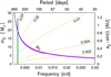 |
Fig. 1 Exoplanet minimum mass m2 as a functionof orbital frequency and different values of a1 sin(i) (labeled in AU, orange lines) orbiting a typical sdB mass ~ 0.5 M⊙. Violet lines represent the values (shown on the right) of the semi-major axes a2 sin (i) of the exoplanetary orbit corresponding to a1 sin(i). The top axis shows the exoplanet orbital period. The green line marks the 0.0024 c/d frequency (referred to later in the text). |
Objects.
3 KIC 9472174: light curves and O−C diagrams
To test and compare the methods, we chose the eclipsing binary KIC 9472174, consisting of a red dwarf and sdBV stars (Table 1; Zola & Baran 2013) as the first target. The star has been intensively investigated by Østensen et al. (2010; radial velocity measurements, modeling, and variability of the sdBV component), Barlow et al. (2012; O−C diagrams, primary and secondary minima timings, and binary orbit eccentricity), Zola & Baran (2013; light curve modeling), and Baran et al. (2015; O−C diagrams from prewhitened SC light curve, Jupiter-mass object detection, and asteroseismology). This mKep = 12.26 mag (Kepler filter magnitude) binary has two natural clocks, in the form of a pulsating sdBV star and mid-eclipse times, and both can be used to track time-delays. The claimed Jupiter-mass circumbinary companion orbiting the star at a distance of 0.92 AU with a period of 416 days (Baran et al. 2015) makes the system even more valuable, since it allows us to test the sensitivity of the O−C and time-delay methods on the same object.
3.1 Eclipse-time variations analysis
For our study, we used the Q 5 – Q 17.2 SC data, which have already been analyzed by Baran et al. (2015), as well as Q 1 – Q 4 LC data omitted in previous analyses. Together, these sets of data are hereafter referred to as SC+LC. In order to cross-check the outcomes, we also took Q 0 – Q 17.2 LC light curves from the Villanova catalog (Kirk et al. 2016, normalized flux2), hereafter LC Vill, and processed it the same way as our SC+LC light curve that was extracted from pixel data (see below).
Because SC and LC Kepler data are built up to produce 58.8 s and 29.4 min integrations from 6.02 s exposures (Gilliland et al. 2010), respectively, the 0.12576-day orbital period (Baran et al. 2015) of the binary is covered by ~190 observing points in SC and ~6 points in LC data. This translates into only ~11–13 point coverage of each of the primary minima in the SC light curve, and practically zero or one point coverage of each of the minima in the LC lightcurve. This makes mid-eclipse time calculations using methods such as Kwee-van Woerden (KW; Kwee & van Woerden 1956) vulnerable to any distortions of the shape of the minima, or even impossible in the case of the LC data.
On the other hand, Baran et al. (2015) show that for SC data, the KW method gives results that are consistent with the other methods they used. However, they obtained a smaller scatter in the O−C diagram when they determined the mid-eclipse times by modeling the light curve rather than minima fitting. In our case, instead of a model light curve, we decided to use the template light curve fitting method to find times of minima (Pribulla et al. 2012). Both methods give a similar accuracy for a single minimum time determination. In this work, the template light curve is generated by phase-folding (over the orbital period) and averaging the phased light curve, using a moving average and a 100-point window. This single-period template is then fitted successively to the data to determine the mid-eclipse times.
It turned out that the number of observations covering a single period of the KIC 9472174 binary in the SC datawas enough to fit a one-period long template to the light curve with an average accuracy of ±4 s. However, due to the poor coverage of the light curve by the observations in the LC data, these required a longer template covering several periods to achieve an adequate fit. After a number of trials, we found that the template generated from the LC data should be composed ofat least seven repeated single-period templates. As such, the formal average fitting accuracy of the LC template was close to 50 s. As aresult, from the template fitting, we obtained 8446 SC and 322 LC, and 1514 LC Vill, eclipse-times and calculated O−C diagrams (Figs. 2a and 3a, respectively). A single-period template fit to the SC light curve gives a similar (±3 s) point scatter in the O−C diagram (Fig. 2a), as is seen in the top panel of Fig. 2 of Barlow et al. (2012) and Fig. 4 of Baran et al. (2015). The scatter in the LC part (Fig. 2a) is almost twice as small as the one observed in the SC part.
Since the KIC 9472174 binary system contains a variable sdB star, the pulsations of the sdBV component could be the main cause of the observed point scatter in the O−C diagram. Toreduce this effect, the pulsations can be removed by “prewhitening” the light curves. To do so, following an initial fitting of the templates, the templates were subtracted from the SC+LC and LC Vill data. The residual light curves, which mosly consist of the sdBV pulsations, were prewhitened by simultaneous fitting (in amplitude, frequency, and phase) and subtraction from the residual light curves of identified pulsation modes. All modes with amplitudes higher than 0.02 ppt in the residual light curve were prewhitened.
In the next step, the difference between the residual (after template subtraction) and prewhitened-residual light curves,which represents the pulsation signal in the original data, was subtracted from the original SC+LC andLC Vill data. In this way, the SC+LC and LC Vill light curves were cleaned of pulsations. The pulsation-free light curves were then again fitted with the templates and the new minima-times, as well as O−Cs, were calculated (Figs. 2b and 3b). The overall SC O−C point scatter in Fig. 2b became 30% smaller than the one in Fig. 4 from Baran et al. (2015).
A further decrease in the point scatter in the SC part of the O−C diagram was achieved from a seven-period template fit to the SC pulsation-free data. The final O−C plot based on seven-period fits to both SC and LC light curves is presented in Fig. 2b. All (Figs. 2 and 3) diagrams were calculated for the BJD = 2 454 953.64324 + Epoch⋅0.125765282 ephemeris.
The bottom diagrams shown in Figs. 2c and 3c present the O−C diagrams from each panel b, detrended of the ~1430 and ~1310 day variations for the SC+LC and LC Vill data, respectively. In Figs. 2c and 3c the 416 day O−C variations given by Baran et al. (2015) in their Fig. 3 O−C are shown; they attributed them to the presence of an exoplanet around KIC 9472174. As we can see, the overall time course of the SC+LC O−C in Fig. 2c mostly follows the black sinusoidal line, while the LC Vill O−C Fig. 3c diagram differs drastically.
To evaluate the differences, we compared FT amplitude spectra calculated for both our own O−C diagram and that from Baran et al. (2015). Since the sampling rate for the SC part of the O−C is equal to the orbital period, the Nyquist frequency is ~4 c/d (half of the orbital frequency 7.9513 c/d). Consequently, the FT amplitude spectra were calculated between 0 – 4 c/d and presented in Fig. 4. The 4σ FT detection thresholds shown in the figure were calculated between 0.2 and 4 c/d. They are nearly the same (~0.1 s) for both our and the Baran et al. (2015) O−C FTs.
The FT calculated for the O−C from Baran et al. (2015) has more high frequency peaks (for example at 0.6, 0.73, 0.75, 2.2, 2.6, and 3.0 c/d), which are reduced in amplitude or not present in our FT. Enlargements of the low (0 – 0.012 c/d) frequency regions from Fig. 4 are shown in Fig. 5. The FTs of the LC Vill (left) and combined SC+LC (right) O–Cs in Fig. 5 are over-plotted on top of the Baran et al. (2015) O−C diagram FTs. The bottom panels of Fig. 5 present the FTs of the O–Cs that were prewhitened for the longest 1310 and 1430 day trends that are visible in the top panels at 0.000764 c/d (LC Vill) and 0.000707 c/d (SC+LC), respectively, as well as the 1114 day trend in (Baran et al. 2015) O−C FT at 0.000898 c/d. The orbital frequency of the putative planetary candidate from Baran et al. (2015) are marked at 0.0024 c/d. The remaining highest-amplitude signals at 0.00256 ± 0.00002 c/d and 0.00238 ± 0.00003 c/d for LC Vill and SC+LC O−Cs (bottom panels of Fig. 5), respectively, are close in frequencies to the 0.00240 ± 0.00001 c/d frequency found by Baran et al. (2015). However, the 0.73 ± 0.04 s amplitude of the LC Vill O−C signal is nearly twice as low as the 1.21 ± 0.02 s amplitude of the signal reported by Baran et al. (2015), while the amplitude of SC+LC O−Cs 0.36 ± 0.03 s is beyond the FT detection threshold.
This indicates a problem with previous interpretations of the signal visible at 0.0024 c/d in the Baran et al. (2015) O−C. Our data analysis shows that the O−C amplitude variations are sensitive to the treatment of the Kepler data before the O−C diagrams are calculated, and it suggests that the signal visible in the Baran et al. (2015) data is a consequence of the data extraction and processing. We notice that the ~416 day periodicities are also observed in the amplitude modulations of the pulsation modes (see Baran et al. 2015, Fig. 2 for the FT amplitude spectra of the KIC 9472174 pulsation modes). For some modes, their amplitude modulation can be extremely high and pulsations in these modes vanish periodically. The amplitude modulation does not, by itself, have a direct impact on the O–C; however, when it occurs, the data reduction process or residual light curve processing may introduce changes to the shape of the light curve and thus affect the resulting measurements of the mid-eclipse times.
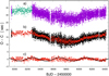 |
Fig. 2 KIC 9472174: O−C diagrams calculated from: (a) SC and LC data (violet and green dots, respectively), and (b) data prewhitened from pulsations (black dots are the O−C from the single-template fit to the SC data; red dots represent the O−C from the seven-period template fit to the SC+LC data). The diagrams were shifted vertically to avoid overlapping. Bottom panel (c): O−C diagram from a seven-period template fit prewhitened for the 1430 day period. The black line shows a 416 day sinusoidal fit to the O−C from Fig. 3 of Baran et al. (2015). |
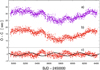 |
Fig. 3 KIC 9472174: O−C diagrams calculated from seven-period template fits to (a): the original LC Vill data, and (b): LC Vill data prewhitened from pulsations. The diagrams were shifted vertically for better visibility. Bottom panel (c): O−C shown at (b) prewhitened for the longest 1310 day period. The black line shows a 416 day sinusoidal fit to the O−C from Fig. 3 of Baran et al. (2015). |
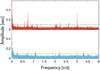 |
Fig. 4 KIC 9472174: O−C FTs for SC Baran et al. (2015) O−C (top) and this work (bottom). Horizontal lines mark 4σ FT detection thresholds. |
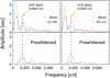 |
Fig. 5 KIC 9472174: enlargement of 0 – 0.012 c/d FT-frequency region from Fig. 2. Red lines: SC Baran et al. (2015) data. Blue lines: this work, LC Villanova data (left panels), and SC+LC data (right panels). Top: O−C FTs before prewhitening. Bottom: after prewhitening the O−Cs for the longest periods. Vertical dashed lines at 0.0024 c/d show the orbital frequency location of the putative exoplanet. |
3.2 Binarograms
KIC 9472174 has two natural clocks which can be used. One is the 7.9513 c/d orbital frequency of the eclipsing binary itself, and the other is in the form of the pulsation modes of the sdBV component, which is determined from the FT amplitude spectrum of the residual light curve described above.
Using the orbital frequency of a binary to determine its time-delay variation is novel, but quite easy to do. We took the pulsation-free binary light curve (see above) and following the recipe given by Balona (2014), using a 4 day window and 2 day stepping time, we calculated the binarogram between 0 – 1 c/d. Initially it had a lot of artifacts, which disappeared after we included the first harmonic (15.9026 c/d) of the orbital frequency in the calculation. The resulting binarogram is featureless; the only signal we found is located below 0.0015 c/d and is due to the variable orbital frequency (Balona 2014, Fig. 8). For better visibility, we show a fraction of the orbital frequency binarogram between 0 – 0.03 c/d in Fig. 6.
The binarogram shows values of a1 sin(i), where a1 is the length of the semi-major axis of the orbit of the binary component of mass m1 around the center of mass of the system and a third body of mass m3 (i is the inclination toward the observer of the third body’s orbit). Given that the orbital frequency of the third body derived from the binarogram is error-less, one solves the nonlinear least-squares problem (Balona 2014, Eqs. (1)–(4)) for a1 sin (i), and all of the uncertainty in the binarogram is attached to a1 sin(i). However, the estimated error for a1 sin(i) from the least-squares solution is the lowest uncertainty by far. The main difficulty with the binarogram arises when the frequency of the clock used to measure the time-delay is unstable, or if there is interference from different pulsation frequencies. Therefore, any noise in the binarogram is mainly due to these two effects. In practice, to find real signals in the binarogram, we use the same technique as for finding signals in the FT of the light curve, that is, by calculating the mean noise (σ) of the binarogram and setting the detection threshold at a certain σ level. Here we set the detection threshold to 4 σ. Since the mean noise in the orbital frequency binarogram is equal to 0.0005 AU (calculated between 0 and 0.03 c/d), the detection threshold is 0.002 AU (Fig. 6, top panel).
Now, if we consider m1 and m3 to be 0.6 M⊙ (Table 1) and ~0.002 M⊙, respectively, and for the semi-major axis of the third body orbit to be a3 ≈ 0.9 AU, the third body orbital frequency to be 0.0024 c/d (Baran et al. 2015), and the orbital inclination of m3 to be the same as the binary orbit of KIC 9472174, that is, i ≈ 69° (Baran et al. 2015), the signal amplitude would be at ~0.0028 AU. Including the binarogram noise of 0.0005 AU (see above), error propagation provides a lower limit of ~0.0023 AU for the signal amplitude. This is still above the 0.002 AU binarogram detection threshold. Consequently, we cannot confirm the existence of an exoplanet on a 416 day orbit (at 0.9 AU distance) around the binary system and with a minimum mass of 0.002 M⊙, as claimed by Baran et al. (2015).
Since the actual a1 sin(i) error in the binarogram cannot be directly calculated, there might be some doubts whether a real exoplanetary signal, if it existed, would be detectable using this method on the data we have. Therefore, we prepared a synthetic light curve with induced time-delays from the putative exoplanet on a 416-day circular orbit around the binary at a distance of 0.9 AU from the star and orbital inclination i = 69° toward the observer. The flux from the binary was simulated by generating a sinusoidal light curve of the same frequency and amplitude as observed in the FT of the real binary light curve (i.e., 7.951319984 c/d and 63 ppt, respectively), and a spacing between synthetic light curve points which exactly mimicked the time distribution of the observed points in the real data for KIC 9472174. We then calculated orbital frequency binarograms as described above for both for the noiseless synthetic light curve Fig. 7 and with the addition of noise at the 3 ppt level (same figure). This is more than the 1 ppt standard deviation of the real data (which contains flux from the pulsating sdBV component) calculated from the ten-point moving average.
As we can see for the noiseless synthetic light curve, the binarogram signal-amplitude a1 sin(i) and orbital frequency are reproduced exactly as introduced to the light curve (see the binarogram maximum at 0.0028 AU and 0.0024 c/d in Fig. 7). Adding noise to the synthetic light curve causes a signal-amplitude decrease from 0.0028 to 0.0027 AU, while the orbital frequency remains the same. The binarogram noise is also reproduced at the ~0.0005 AU level, as it is in the orbital frequency binarogram calculated from the real data (Fig. 6). As a result, the binarogram derived from synthetic data gives a detection threshold at the same level as observed in the real data. We also note that changes in the binary orbital frequency adopted for the binarogram calculations result in an artifact signal below 0.0015 c/d, which is similar to the one observed in Fig. 6. This sets a ~800-day limit on the longest orbital periods, which can be traced using the data we have. Taking the real and simulated data analysis into account, we can state that there is no exoplanet around the binary star KIC 9472174 with the orbital parameters and minimum mass inferred by Baran et al. (2015).
Whether or not we can do the same thing using pulsation modes needs to be determined. As mentioned earlier, the main difficulty in calculating binarograms based on stellar pulsations is the interference between neighboring close pulsation frequencies and pulsation mode amplitude or frequency variations. The interference (or other pulsation mode variations) in frequencies result in binarogram artifacts, which must be distinguished from real signals. To do so, one needs to calculate binarograms for a few different sets of pulsation frequencies or data sets, for example by dividing the light curve into two or more parts and comparing the resulting binarograms with each other. The real signal is present at the same frequency and with a similar amplitude in all of the binarograms. This procedure requires a lot of computation time depending on the data length and the number of frequencies used. In the case of the SC Kepler light curve, ~1.5 million points and ~20–30 pulsation modes, it takes about 24 h to calculate a binarogram within a 1 c/d orbital frequency range.
In the bottom panel of Fig. 6, we present example binarograms calculated for the KIC 9472174 SC data and three frequency sets: one consisting of 14 frequencies; another with the highest 195.7661 c/d amplitude mode; and the last one with the second highest amplitude 40.0265 c/d mode. As we can see, all signals below 0.005 c/d differ in amplitude and frequencies and should be regarded as artifacts. Another signal at ~0.026 c/d has the same frequency for all three binarograms; however, for one set of frequencies, its amplitude is ~40% smaller. This suggests it is also not a real signal. As we mentioned earlier, the main difficulties in the pulsation-frequency binarograms are pulsation frequency variations and frequency interference, which cause an increase in binarogram noise and result in artifact signals. In this case, the detection threshold of the pulsation-frequency binarogram (bottom panel of Fig. 6) is ~0.026 AU. It is an order of magnitude greater than the one calculated for the orbital frequency binarogram, and we cannot reach the detectability required for the reliable detection of the putative exoplanet.
In summary, the example of KIC 9472174 shows that the data treatment can greatly influence the final shape of the O−C diagram and the conclusions drawn. However, the orbital frequency binarogram was sensitive enough to rule out the existence of the planetary companion suggested by Baran et al. (2015). In fact, by using this binarogram, we could have detected a minimum ~1.5 MJ mass object at a distance of 0.9 AU from the binary on a 416-day orbit inclined at i = 69°, if it existed, or an ~2 MJ mass object on orbit inclined at i = 43°.
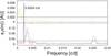 |
Fig. 6 KIC 9472174: binarograms calculated using the orbital frequency of the eclipsing binary (top panel, the vertical black line shows the orbital frequency of the putative exoplanet) and using different pulsation frequency sets of the sdBV component (bottom panel). Red represents the set of 14 frequencies; green is the highest amplitude mode; and violet is the second high amplitude mode. |
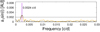 |
Fig. 7 KIC 9472174: orbital frequency binarograms calculated from the synthetic light-cuves for the noiseless data (black line) and forthe data with 3 ppt noise added (orange line). Vertical (violet) and horizontal (black) lines show the orbital frequency of the putative exoplanet and the 0.002 AU detection threshold, respectively. |
4 KIC 7975824: O−C and binarogram
The O−C analysis and binarogram of another eclipsing binary system composed of sdB and WD stars is presented in this section. The orbital period of this star is longer, 0.40375026 d (see Table 1), and the star is fainter (mKep = 14.66 mag) than the previous one. The analysis was performed on joined Q 1, Q 5 – Q12 SC, and Q13 – Q 17.2 LC data (SC+LC). The SC+LC light curves were obtained the same way as described above. The fluxes and FT of the residual SC+LC light curve were calculated from single- and twenty-period template fits to the SC and LC light curves, respectively. The FT does not show any real periodic signals. The only features above the 0.008 ppt FT detection threshold are some remnant signals around the orbital frequency and six known Kepler artifacts at 440.43, 391.49, 342.55, 489.36, 685.11, and 734.04 c/d (in order of decreasing amplitude). Therefore, we can confirm the finding by Bloemen et al. (2011) that neither of the binary components are intrinsically variable down to this detection threshold.
The mid-times of eclipses were calculated from the template fits to the light curve and the resulting O−C diagram is presented in the top panel of Fig. 8. The diagram was calculated for the ephemeris BJD = 2 454 964.52672 + Epoch ⋅ 0.403750221 day, derived from a linear fit to the SC+LC minima times.
It can be seen that the points on the O−C diagram in the top panel of Fig. 8 are scattered by about ± 50 s around zero (standard deviation ±17 s). Open squares at the end of the O−C diagram represent points obtained from a twenty-period template fit to the LC light curve. As far as we can tell, there are no variations in the diagram. In the bottom panel of the figure, we also show the O−C FT, which confirms that the orbital period was stable during the whole time of observation.
In the next step, we calculated the binarogram from the SC+LC light curve (Fig. 9), using the binary orbital frequency as a clock. Since the KIC 797582 system is more massive (1.06 M⊙, Table 1), we expect a lower sensitivity in the binarogram than was the case for the previous star. The binarogram detection threshold visible in Fig. 9 is about 0.048 AU, allowing for the detection of 0.05 M⊙ bodies on a ~1 AU orbit around the system in the best conditions (i ≈ 90°). The low sensitivity is apparently due to the higher mass of the system, the smaller amplitude of the light curve variations, and the larger noise in the data compared to the KIC 9472174 light curve.
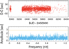 |
Fig. 8 KIC 7975824: O−C diagram (top) and its FT (bottom). The orange line in the bottom panel marks the 4σ FT detection threshold. |
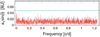 |
Fig. 9 KIC 7975824: orbital frequency binarogram. The horizontal line marks the 4σ FT detection threshold. |
5 KIC 862602: binarogram of a pulsating WD star
KIC 8626021 is a mKep = 18.46 mag pulsating helium atmosphere white dwarf (DBV), showing about 12 pulsation frequencies in its light curve FT (Zong et al. 2016; Giammichele et al. 2018). This time, however, we have a single pulsating star and only the time-delay method can be used to search for substellar bodies orbiting the WD. As the mass of KIC 8626021 is 0.55 M⊙, for a 0.002 M⊙ object orbiting the DBV star at a distance of 1 AU, one can therefore expect the binarogram signal to be ~ 0.0036 AU at best.
For the analysis, Q 10 – Q 17.2 SC data were downloaded from MAST and the SC light curve was extracted as described in Sect. 2. The archive contains Q 7 of LC, but it was not included since the LC data cannot follow the high frequency signals found in pulsating WDs. For the binarogram calculation, the pulsation mode frequencies were taken from Zong et al. (2016), who analyze the pulsation properties of the star in detail. However it turns out that, due to the variation of the amplitudes and phases of the pulsation frequencies and the presence of multiplets, the resulting binarograms are contaminated by a number of artifacts near 0.275, 0.29, 0.55, 0.58, 2.15, and 2.4 c/d (Fig. 10). We note that these binarograms were calculated for a wider orbital frequency range 0–3.5 c/d (Fig. 10, top panel) than for the previous two stars in order to demonstrate the issue, and the main part of our analysis consisted of ruling these artifacts out.
To do so, binarograms were calculated for different sets of frequencies as well as for the two halves of the data. Since a real a1 sin(i) signal should be independent of the subsets of data and frequency used for the calculations, the real signal should appear at the same frequency and amplitude in each binarogram, with an accuracy corresponding to the binarogram resolution and its noise level. In our case, the binarogram noise is at ~0.00125 AU in Fig. 10; therefore, real signal amplitude variations can differ by approximately this amount for different subsets of the data. Different line colors in the figure represent binarograms calculated for different sets of pulsation frequencies. The regions around two pairs of strong signals near 0.4 and 2.25 c/d of the top panel were enlarged in the frequency range and are presented inlower panels of Fig. 10. One can clearly see in the bottom panels that all the visible signal frequencies or amplitudes differ considerably; therefore, all of them can be classified as artifacts. The detection threshold drops down to 0.004 AU for some sets of frequencies and this sets the minimum mass limit for a substellar object, which could be found at a distance of ~1 AU to about 2–3 MJ, assuming i = 90° (see Fig. 1).
In summary, the low detection threshold of the pulsation-based binarogram allows us to search for substellar objects of the lowest (0.002 M⊙) masses at a distance of 1 AU from a WD. The noise level can be surprisingly small, even for pulsation-mode binarograms and faint stars.
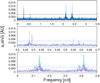 |
Fig. 10 KIC 8626021: binarograms for different pulsation frequency sets (different line colors). Bottom panels: enlargements of two artifact regions around 0.27 c/d and 2.3 c/d from the top panel. We note that the detection threshold changes (horizontal lines near ~0.004 AU) depending on the frequency sets used to calculate the binarograms. |
6 Conclusions
Using time-delay, FT and O−C methods, we analyzed the light curves of two binaries and one pulsating WD. By comparing our O−C diagrams tothose of Baran et al. (2015), we find no evidence for the claimed Jupiter-mass planet at ~0.9 AU from the binary. We found that the ~391 day cycle of variations observed in the LC Vill O−C (Fig. 3c) is in antiphase to the 416 day variations visible in the Baran et al. (2015) O−C diagram, while variations in the SC+LC O−C diagram are below the detection threshold (Fig. 5). The shape of the final O−C depends on the data reduction techniques and light curve processing.
The O−C diagram is not the definitive method of searching for orbiting companions to eclipsing binaries. Our final conclusion was drawn from the KIC 9472174 binarogram (Fig. 6, top panel). This binarogram was based on the orbital frequency of the system and was sensitive enough to rule out the presence of a Jupiter- or higher-mass object on a 0.9 AU and 416-day orbit (i ≈ 69°) around the star, such as is claimed by Baran et al. (2015). The only possibility for our technique missing this planet would be an orbital inclination lower than 43°. Our conclusion supplements the work by Pulley et al. (2018) based on recent observations of seven sdB systems. The authors show that period variations of these stars cannot be explained simply on the basis of third bodies orbiting these systems. Out of seven binaries studied by authors, only three candidates support the circumbinary object hypothesis.
We have also shown that the binarogram detection threshold depends on various factors, that is, light curve noise, an amplitude of light variations, and the stability of pulsation frequencies. However, the final detection threshold is difficult to predict. In the case of the bright eclipsing binary KIC 9472174, the lowest noise level was achieved for the orbital-frequency binarogram; whereas, for the pulsation-mode binarogram, the noise was ten times higher. On the other hand, the noise level of the pulsation-frequency binarogram of the single WD, KIC 8626021, which is a rather faint star, was comparable to that seen in the orbital-frequency binarogram of the binary KIC 9472174. Additional problems are generated by artifacts. In the orbital frequency binarogram, the artifacts can be removed by the inclusion of orbital frequency harmonics (usually the first is enough) into the calculation. However, artifacts in pulsation-mode binarograms can only be distinguished from real signals by comparing many binarograms calculated for different subsets of frequencies or data.
The methods we used are, in some cases, sensitive enough to search for giant planets around WDs, sdBs, and short period eclipsing binaries. While data from the primary part of the Kepler telescope mission allows for these types of searches to be performed for longer ~800-day orbital periods (i.e., larger, up to ~1.4 AU, distances from the stars) and ~1 MJ exoplanets, the K2 SC light curves (~80 day photometric time-series data) restrict the search to short, 10–40 day periods and therefore to 7–20 MJ and higher mass objects.
Acknowledgements
This work was supported by the National Science Centre, Poland. The project registration number is 2017/25/B/ST9/00879. The authors would like to thank Luis Balona from South African Astronomical Observatory, who kindly provided hissoftware.
References
- Baglin, A., Breger, M., Chevalier, C., et al. 1973, A&A, 23, 221 [NASA ADS] [Google Scholar]
- Balona, L. A. 2014, MNRAS, 443, 1946 [NASA ADS] [CrossRef] [Google Scholar]
- Baran, A. S., Zola, S., Blokesz, A., Østensen, R. H., & Silvotti, R. 2015, A&A, 577, A146 [NASA ADS] [CrossRef] [EDP Sciences] [Google Scholar]
- Barlow, B. N., Wade, R. A., & Liss, S. E. 2012, ApJ, 753, 101 [NASA ADS] [CrossRef] [Google Scholar]
- Bear, E., & Soker, N. 2014, MNRAS, 437, 1400 [NASA ADS] [CrossRef] [Google Scholar]
- Bloemen, S., Marsh, T. R., Østensen, R. H., et al. 2011, MNRAS, 410, 1787 [NASA ADS] [Google Scholar]
- Blokesz, A., Krzesinski, J., & Kedziora-Chudczer, L. 2019, A&A, 627, A86 [CrossRef] [EDP Sciences] [Google Scholar]
- Borucki, W. J., Koch, D., Basri, G., et al. 2010, Science, 327, 977 [NASA ADS] [CrossRef] [PubMed] [Google Scholar]
- Bours, M. C. P., Marsh, T. R., Parsons, S. G., et al. 2016, MNRAS, 460, 3873 [NASA ADS] [CrossRef] [Google Scholar]
- Brown, T. M., Latham, D. W., Everett, M. E., & Esquerdo, G. A. 2011, AJ, 142, 112 [NASA ADS] [CrossRef] [Google Scholar]
- Cassan, A., Kubas, D., Beaulieu, J. P., et al. 2012, Nature, 481, 167 [NASA ADS] [CrossRef] [Google Scholar]
- Charpinet, S., Fontaine, G., Brassard, P., et al. 2011, Nature, 480, 496 [NASA ADS] [CrossRef] [PubMed] [Google Scholar]
- Conroy, K. E., Prša, A., Stassun, K. G., et al. 2014, AJ, 147, 45 [NASA ADS] [CrossRef] [Google Scholar]
- Gänsicke, B. T., Schreiber, M. R., Toloza, O., et al. 2019, Nature, 576, 61 [NASA ADS] [CrossRef] [Google Scholar]
- Geier, S., Edelmann, H., Heber, U., & Morales-Rueda, L. 2009, ApJ, 702, L96 [NASA ADS] [CrossRef] [Google Scholar]
- Giammichele, N., Charpinet, S., Fontaine, G., et al. 2018, Nature, 554, 73 [NASA ADS] [CrossRef] [Google Scholar]
- Gilliland, R. L., Jenkins, J. M., Borucki, W. J., et al. 2010, ApJ, 713, L160 [NASA ADS] [CrossRef] [Google Scholar]
- Heber, U. 2016, PASP, 128, 082001 [NASA ADS] [CrossRef] [Google Scholar]
- Hermes, J. J. 2018, Handbook of Exoplanets, eds. H. Deeg, & J. Belmonte (Cham: Springer), 787 [CrossRef] [Google Scholar]
- Jones, M. I., & Jenkins, J. S. 2014, A&A, 562, A129 [NASA ADS] [CrossRef] [EDP Sciences] [Google Scholar]
- Kirk, B., Conroy, K., Prša, A., et al. 2016, AJ, 151, 68 [NASA ADS] [CrossRef] [Google Scholar]
- Krzesinski, J. 2015, A&A, 581, A7 [NASA ADS] [CrossRef] [EDP Sciences] [Google Scholar]
- Krzesinski, J., Blokesz, A., Ogłoza, W., & Dróżdż, M. 2020, IAU Symp., 345, 306 [Google Scholar]
- Kwee, K. K., & van Woerden, H. 1956, Bull. Astron. Inst. Netherlands, 12, 327 [Google Scholar]
- Murphy, S. J. 2012, MNRAS, 422, 665 [NASA ADS] [CrossRef] [Google Scholar]
- Murphy, S. J., & Shibahashi, H. 2015, MNRAS, 450, 4475 [NASA ADS] [CrossRef] [Google Scholar]
- Østensen, R. H., Green, E. M., Bloemen, S., et al. 2010, MNRAS, 408, L51 [NASA ADS] [CrossRef] [Google Scholar]
- Pribulla, T., Vaňko, M., Ammler-von Eiff, M., et al. 2012, Astron. Nachr., 333, 754 [NASA ADS] [CrossRef] [Google Scholar]
- Pulley, D., Faillace, G., Smith, D., Watkins, A., & von Harrach, S. 2018, A&A, 611, A48 [NASA ADS] [CrossRef] [EDP Sciences] [Google Scholar]
- Rasio, F. A., Tout, C. A., Lubow, S. H., & Livio, M. 1996, ApJ, 470, 1187 [NASA ADS] [CrossRef] [Google Scholar]
- Setiawan, J., Klement, R. J., Henning, T., et al. 2010, Science, 330, 1642 [NASA ADS] [CrossRef] [Google Scholar]
- Shibahashi, H., & Kurtz, D. W. 2012, MNRAS, 422, 738 [NASA ADS] [CrossRef] [Google Scholar]
- Silvotti, R., Schuh, S., Janulis, R., et al. 2007, ASP Conf. Ser., 372, 369 [Google Scholar]
- Silvotti, R., Charpinet, S., Green, E., et al. 2014, A&A, 570, A130 [NASA ADS] [CrossRef] [EDP Sciences] [Google Scholar]
- Staff, J., De Marco, O., Wood, P., Galaviz, P., & Passy, J.-C. 2016, MNRAS, 458, 832 [NASA ADS] [CrossRef] [Google Scholar]
- Sterken, C. 2005, ASP Conf. Ser., 335, 3 [Google Scholar]
- Vanderburg, A., & Rappaport, S. A. 2018, Handbook of Exoplanets, eds. H. Deeg, & J. Belmonte (Cham: Springer), 2603 [CrossRef] [Google Scholar]
- Veras, D., Mustill, A. J., Gänsicke, B. T., et al. 2016, MNRAS, 458, 3942 [Google Scholar]
- Zola, S., & Baran, A. 2013, Central Eur. Astrophys. Bull., 37, 227 [Google Scholar]
- Zong, W., Charpinet, S., Vauclair, G., Giammichele, N., & Van Grootel, V. 2016, A&A, 585, A22 [NASA ADS] [CrossRef] [EDP Sciences] [Google Scholar]
All Tables
All Figures
|
Fig. 1 Exoplanet minimum mass m2 as a functionof orbital frequency and different values of a1 sin(i) (labeled in AU, orange lines) orbiting a typical sdB mass ~ 0.5 M⊙. Violet lines represent the values (shown on the right) of the semi-major axes a2 sin (i) of the exoplanetary orbit corresponding to a1 sin(i). The top axis shows the exoplanet orbital period. The green line marks the 0.0024 c/d frequency (referred to later in the text). |
| In the text | |
|
Fig. 2 KIC 9472174: O−C diagrams calculated from: (a) SC and LC data (violet and green dots, respectively), and (b) data prewhitened from pulsations (black dots are the O−C from the single-template fit to the SC data; red dots represent the O−C from the seven-period template fit to the SC+LC data). The diagrams were shifted vertically to avoid overlapping. Bottom panel (c): O−C diagram from a seven-period template fit prewhitened for the 1430 day period. The black line shows a 416 day sinusoidal fit to the O−C from Fig. 3 of Baran et al. (2015). |
| In the text | |
|
Fig. 3 KIC 9472174: O−C diagrams calculated from seven-period template fits to (a): the original LC Vill data, and (b): LC Vill data prewhitened from pulsations. The diagrams were shifted vertically for better visibility. Bottom panel (c): O−C shown at (b) prewhitened for the longest 1310 day period. The black line shows a 416 day sinusoidal fit to the O−C from Fig. 3 of Baran et al. (2015). |
| In the text | |
|
Fig. 4 KIC 9472174: O−C FTs for SC Baran et al. (2015) O−C (top) and this work (bottom). Horizontal lines mark 4σ FT detection thresholds. |
| In the text | |
|
Fig. 5 KIC 9472174: enlargement of 0 – 0.012 c/d FT-frequency region from Fig. 2. Red lines: SC Baran et al. (2015) data. Blue lines: this work, LC Villanova data (left panels), and SC+LC data (right panels). Top: O−C FTs before prewhitening. Bottom: after prewhitening the O−Cs for the longest periods. Vertical dashed lines at 0.0024 c/d show the orbital frequency location of the putative exoplanet. |
| In the text | |
|
Fig. 6 KIC 9472174: binarograms calculated using the orbital frequency of the eclipsing binary (top panel, the vertical black line shows the orbital frequency of the putative exoplanet) and using different pulsation frequency sets of the sdBV component (bottom panel). Red represents the set of 14 frequencies; green is the highest amplitude mode; and violet is the second high amplitude mode. |
| In the text | |
|
Fig. 7 KIC 9472174: orbital frequency binarograms calculated from the synthetic light-cuves for the noiseless data (black line) and forthe data with 3 ppt noise added (orange line). Vertical (violet) and horizontal (black) lines show the orbital frequency of the putative exoplanet and the 0.002 AU detection threshold, respectively. |
| In the text | |
|
Fig. 8 KIC 7975824: O−C diagram (top) and its FT (bottom). The orange line in the bottom panel marks the 4σ FT detection threshold. |
| In the text | |
|
Fig. 9 KIC 7975824: orbital frequency binarogram. The horizontal line marks the 4σ FT detection threshold. |
| In the text | |
|
Fig. 10 KIC 8626021: binarograms for different pulsation frequency sets (different line colors). Bottom panels: enlargements of two artifact regions around 0.27 c/d and 2.3 c/d from the top panel. We note that the detection threshold changes (horizontal lines near ~0.004 AU) depending on the frequency sets used to calculate the binarograms. |
| In the text | |
Current usage metrics show cumulative count of Article Views (full-text article views including HTML views, PDF and ePub downloads, according to the available data) and Abstracts Views on Vision4Press platform.
Data correspond to usage on the plateform after 2015. The current usage metrics is available 48-96 hours after online publication and is updated daily on week days.
Initial download of the metrics may take a while.