| Issue |
A&A
Volume 649, May 2021
|
|
|---|---|---|
| Article Number | A25 | |
| Number of page(s) | 10 | |
| Section | Interstellar and circumstellar matter | |
| DOI | https://doi.org/10.1051/0004-6361/201936787 | |
| Published online | 07 May 2021 | |
Possible single-armed spiral in the protoplanetary disk around HD 34282★,★★
1
Leiden Observatory, Leiden University,
PO Box 9513,
2300
RA Leiden, The Netherlands
2
Sterrenkundig Instituut Anton Pannekoek,
Science Park 904,
1098 XH
Amsterdam, The Netherlands
e-mail: c.ginski@uva.nl
3
Univ. Grenoble Alpes, CNRS, IPAG,
38000
Grenoble, France
4
ASML, De Run 6501,
5504 DR
Veldhoven, The Netherlands
5
Space Telescope Science Institute,
Baltimore,
MD
21218, USA
6
INAF, Osservatorio Astrofisico di Arcetri,
Largo Enrico Fermi 5,
50125
Firenze, Italy
7
LESIA, Observatoire de Paris, Université PSL, CNRS, Sorbonne Université, Univ. Paris Diderot, Sorbonne Paris Cité,
5 place Jules Janssen,
92195
Meudon,
France
8
Institute for Particle Physics and Astrophysics, ETH Zurich,
Wolfgang-Pauli-Strasse 27,
8093
Zurich, Switzerland
9
Lakeside Labs,
Lakeside Park B04b,
9020
Klagenfurt, Austria
10
Aix Marseille Université, CNRS, CNES, LAM,
Marseille, France
11
Max Planck Institute for Astronomy,
Königstuhl 17,
69117
Heidelberg, Germany
12
NOVA Optical Infrared Instrumentation Group,
Oude Hoogeveensedijk 4,
7991 PD
Dwingeloo, The Netherlands
13
DOTA, ONERA, Université Paris Saclay,
91123
Palaiseau,
France
Received:
25
September
2019
Accepted:
22
October
2020
Context. During the evolution of protoplanetary disks into planetary systems we expect to detect signatures that trace mechanisms such as planet–disk interaction. Protoplanetary disks display a large variety of structures in recently published high-spatial resolution images. However, the three-dimensional morphology of these disks is often difficult to infer from the two-dimensional projected images we observe.
Aims. We aim to detect signatures of planet–disk interaction by studying the scattering surface of the protoplanetary disk around HD 34282.
Methods. We spatially resolved the disk using the high-contrast imager VLT/SPHERE in polarimetric imaging mode. We retrieved a profile for the height of the scattering surface to create a height-corrected deprojection, which simulates a face-on orientation.
Results. The detected disk displays a complex scattering surface. An inner clearing or cavity extending up to r < 0.′′28 (88 au) is surrounded by a bright inclined (i = 56°) ring with a position angle of 119°. The center of this ring is offset from the star along the minor axis with 0.′′07, which can be explained with a disk height of 26 au above the midplane. Outside this ring, beyond its southeastern ansa we detect an azimuthal asymmetry or blob at r ~ 0.′′4. At larger separation, we detect an outer disk structure that can be fitted with an ellipse, which is compatible with a circular ring seen at r = 0.′′62 (=190 au) and a height of 77 au. After applying a height-corrected deprojection we see a circular ring centered on the star at 88 au; what had seemed to be a separate blob and outer ring could now both be part of a single-armed spiral.
Conclusions. We present the first scattered-light image of the disk around HD 34282 and resolve a disk with an inner cavity up to r ≈ 90 au and a highly structured scattering surface of an inclined disk at a large height Hscat∕r = 0.′′29 above the midplane at the inner edge of the outer disk. Based on the current data it is not possible to conclude decisively whether Hscat∕r remains constant or whether the surface is flared with at most Hscat ∝ r1.35, although we favor the constant ratio based on our deprojections. The height-corrected deprojection allows for a more detailed interpretation of the observed structures, from which we discern the first detection of a single-armed spiral in a protoplanetary disk.
Key words: protoplanetary disks / planet–disk interactions / planets and satellites: formation / circumstellar matter / stars: pre-main sequence / polarization
The reduced images are also available at the CDS via anonymous ftp to cdsarc.u-strasbg.fr (130.79.128.5) or via http://cdsarc.u-strasbg.fr/viz-bin/cat/J/A+A/649/A25
© ESO 2021
1 Introduction
The study of planet formation in protoplanetary disks has reached a new era with the possibility of imaging these disks at a high angular resolution. The developments at both the optical and submillimeter regime have yielded improvements both in obtainable resolution and in sensitivity. In the visible and near-infrared (NIR), the extreme adaptive optics (AO) high-contrast imagers Gemini Planet Imager (Gemini/GPI; Macintosh et al. 2014) and the Spectro-Polarimetric High-contrast Exoplanet REsearch (VLT/SPHERE; Beuzit et al. 2019) instruments reach close to diffraction limited resolutions of ~ 50 ms (mas). These visible and NIR imagers detect light that is scattered by ~ micron (μm) sized dust grains on the disk surface. Long baseline observations at submillimeter wavelengths with the Atacama Large Millimeter Array (ALMA) trace thermal emission of gas and roughly millimeter-sized dust grains in disks at similar (< 0.1′′) resolutions (ALMA Partnership 2015).
Previous assumptions of smooth continuous disks are challenged by high-resolution images with the detection of spiral arms (Muto et al. 2012; Grady et al. 2013; Benisty et al. 2017), gaps, and rings (Quanz et al. 2013; ALMA Partnership 2015; de Boer et al. 2016). While the presence of planets is often considered to be the cause of such structured disks (Ogilvie & Lubow 2002; Dong et al. 2016; de Juan Ovelar et al. 2013), multiple explanations exist for the different types of structure. Among other explanations, disk gaps and cavities can also be caused by the presence of dead zones (Flock et al. 2015; Pinilla et al. 2016)or photoevaporation (Alexander et al. 2006), while spiral arms can be due to self-gravity in the disk (Lodato & Rice 2004; Dipierro et al. 2015) or due to temperature gradients caused by shadowing (Montesinos et al. 2016).
To date, almost exclusively double- (or multiple-)armed spiral structures have been detected in protoplanetary disks.1 Double-armed spirals typically display very similar contrasts between both arms and the surrounding disks2. Self-gravity and shadowing can readily explain such double-armed spirals. However, spirals induced by a (proto)planet are expected to be either single-armed (outside of the planet location) or double-armed (Zhu et al. 2015; Dong et al. 2015; Miranda & Rafikov 2019). Currently, no protoplanetary disk has been detected with a confirmed single-armed spiral structure. When new pre-main-sequence systems are imaged at high resolution, nearly all of these appear to have distinct particularities. Encountering new disk features allows us to study the various details of the interactions in evolutionary processes, which will ultimately yield a better understanding of the general principles driving disk evolution and the formation of planetary systems.
HD 34282 (alias V1366 Ori) is an interesting candidate to search for structure in the protoplanetary disk surrounding this Herbig Ae star (Merín et al. 2004, Spectral type: A3V,). Merín et al. (2004) determined the stellar age at 6.4 ± 0.5 Myr and mass M⋆ = 1.6 ± 0.3 M⊙, assuming a distance of 348 pc. The second data release (DR2) of Gaia (Gaia Collaboration 2018) constrains the distance to 312 ± 5 pc. Based on Gaia DR2, Vioque et al. (2018) adjusted the stellar age to 6.5
 Myr and M⋆ = 1.45 ± 0.07 M⊙.
The presence of a Keplerian disk surrounding HD 34282 is inferred from its strong IR excess (Sylvester et al. 1996) and double-peaked CO (J = 3–2) emission (Greaves et al. 2000). Piétu et al. (2003) resolved an inclined (i = 56 ± 3°) disk with the IRAM interferometer, and determined a temperature law compatible with a flaring disk heated by the central star. Khalafinejad et al. (2016) used the spectral energy distribution (SED) and marginally resolved Q-band images to create a radiative transfer model of the disk, which predicts a gap of 92 au (at 348 pc, which converts to 82
 au at 112 pc). A 0.24′′ (=75 au) wide cavity is detected in the ALMA band 7 continuum image of van der Plas et al. (2017). In the continuum image with a spatial resolution of 0.1′′ ×0.17′′, the disk is resolved and detected up to 1.15′′ from the star as a ~ 60° inclined ring. Furthermore, the ring contains a “vortex-shaped” asymmetry near the southeastern ansa of the elliptical ring.
Maaskant et al. (2014) list the most famous Herbig Ae/Be stars in order of increasing flux ratio F30 μm∕F13.5 μm, which can be used as a tracer for disk flaring. HD 34282 is placed among the top three most flared disks, below IRS 48 and HD 135344B. Based on the predictions of a large gap and very strong flaring of the disk surface, we expect that HD 34282 harbors an easily detectable disk with clearly resolvable features.
In this study, we used VLT/SPHERE to spatially resolve the scattering surface of the protoplanetary disk of HD 34282. Our SPHERE observations are listed in Sect. 2, followed by a description of the reduction and post-processing of this data in Sect. 3. We present our results and perform a geometrical analysis of the images to reconstruct the disk morphology in Sect. 4. We finish with a brief discussion in Sect. 5 and the conclusions in Sect. 6.
2 Observations
We observed HD 34282 with the VLT/SPHERE InfraRed Dual-beam Imager and Spectrograph (SPHERE/IRDIS; Dohlen et al. 2008)and Integral Field Spectrograph (SPHERE/IFS, Claudi et al. 2008) instruments, using the apodized pupil Lyot coronagraph(ALC_YJH_S; Boccaletti et al. 2008; Martinez et al. 2009) with a diameter of 185 mas and inner working angle of 100 mas (Wilby et al., in prep.).
As part of the guaranteed time observations (GTO) of the disk group within the SPHERE consortium, we observed HD 34282 with IRDIS, using the dual-beam polarimetric imaging mode (IRDIS/DPI; Langlois et al. 2014; de Boer et al. 2020; van Holstein et al. 2020) with a broadband J filter (λ0 = 1.258 μm, Δλ = 197 nm). The IRDIS/DPI observations are recorded on December 19, 2015 with detector integration times (DITs) of 64 s in field-stabilized mode. During the total exposure time of 94 min, we cycled through the four half-wave plate positions (0°, 45°, 22.5°, and 67.5°, to modulatethe linear polarization components) 11 times.
During the GTO of SpHere INfrared survey for Exoplanets (SHINE) on October 25, 2015, we observed HD 34282 in IRDIFS mode: The IFS recorded in Y -J band (λ = 0.96–1.34 μm, with spectral resolution Δλ = 55.1 nm); IRDIS in dual-band imaging mode (DBI; Vigan et al. 2010) with the H2–H3 filter combination (H2: λ0 = 1.5888μm; Δλ = 53.1 nm; H3: λ0 = 1.6671μm; Δλ = 55.6 nm). The SHINE observations with both IRDIS and IFS were recorded in pupil-stabilized mode, using DITs of 64 s for a total exposure time of 68 min, during 54° of field rotation.
3 Data reduction
We reduced the data using the method discussed in detail by de Boer et al. (2016). The linear polarization images are retrieved by computing Stokes vector components Q and U with the double difference method. Next, we determined for each pixel the angle ϕ between the meridian and the line crossing both this pixel and the star center (increasing from north to east). We used the Stokes vector components to determine where the polarization angle at each point in the image is aligned in azimuthal direction with respect to the star center (Qϕ, negative signal represents radial alignment of the polarization direction) and where the polarization angle is aligned ± 45° with respect to the star center (Uϕ) according toSchmid et al. (2006),

In disks seen at near face-on orientation (e.g., TW Hydrae; van Boekel et al. 2017) we can expect the Uϕ signal to be dominated by noise and instrumental or reduction artifacts. However, a study based on radiative transfer modeling by Canovas et al. (2015) showed that due to the breaking of symmetry (of scattering angles) in protoplanetary disks seen at high inclination angles, multiple scattering can cause a true deviation from azimuthal polarization: that is, Uϕ disk signal. Although the inclination of the disk around HD 34282 is known to be high (56–60°), we used the assumption that the disk signal is dominated by single scattering to correct for the reduction artifacts caused by an insufficient instrumental polarization correction. We removed a constant scalar multiplied with the total intensity image from the Q and U images independently, which yielded the lowest absolute signal in the Uϕ image along an annulus centered on the star. In our final images, we corrected for bad pixels by applying a sigma filter. For each pixel in our frame, we measured the standard deviation in a box surrounding (but excluding) this pixel with width of seven pixels. When the central pixel deviates by more than 3σ from the mean of the remaining pixels within the box, it is replaced by this mean value. In accordance with Maire et al. (2016), the resulting Qϕ and Uϕ images are aligned with true north by rotating them by 1.8° in clockwise direction and a pixel scale of 12.26 mas is assumed.
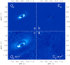 |
Fig. 1 Polarimetric images of HD 34282 by VLT/SPHERE/IRDIS. In all panels, north is up, east is left, and the star center is annotated with a green cross. All images are shown on a linear color map. (a) The Qϕ image showsthe inner cavity, surrounded by the bright inner edge (or wall) of the outer disk as an ellipse with its center slightly offset from the star in the northeastern direction. Faint structures are detected directly outside this inner wall. (b) The Uϕ image shownwith the same intensity range as panel a. (c) To highlight the outer disk structures we scaled the Qϕ image with the disk radius squared, corrected for the inclination (Piétu et al. 2003, 56°). To a first order, this r2 scaling accounts for the decrease in stellar irradiation of the disk. The height of the scattering surface was not taken into account, thus this scaling is only shown for illustrative purpose so as to highlight the fainter structures outside the inner wall. (d) Uϕ with the same r2 scaling and shown for the same intensity range as panel c. |
4 Results and geometrical analysis
We show the final Qϕ and Uϕ images in Figs. 1a, b To highlight the outer disk structures, we multiplied Qϕ and Uϕ in Figs. 1c, d with the square of the separation (r2) to the star, using inclination (i = 56°) and the assumption that the scattering surface has no height above the midplane (thin disk). We realize that the thin-disk assumption is an unlikely simplification. Hence, the inclination corrected r2 scaling is only used for visualization purposes: to simultaneously show the inner and outer disk features. A similar effect of covering a larger dynamical range in an image is reached by showing these features in logarithmic scale, as we do in Fig. 2. The log scale has the benefit that is unbiased by our choice for the inclination and height of the scattering surface, but is unsuitable for a clear display of the Uϕ image (which can have large negative values) and shows the outer regions more diffusely than the r2 -scaled image.
Figure 2 is annotated with the most distinct disk features. At the smallest separations, we detect a clearing in the disk or inner cavity, which is surrounded by a ring feature (R2). Further from the star we detect a second ring-like feature (R1), an arc(A1) below a dark lane in the southwest, an arc (A2) outside the southeastern ansa of R1, a diffuse signal on the opposite side (A3, outside the northwestern ansa of R1), and finally a bright arc or blob (B1) in between the southeastern ansae of R1 and R2.
Previous SED analysis by Maaskant et al. (2014) already shows that the disk is not geometrically thin and most likely flared. Additionally, the disk images of Figs. 1a,c show indications that the thin disk assumption is unlikely to be correct. Therefore, all quantitative analyses below are performed on the non-scaled image (Fig. 1a). The first indication in our data that the thin-disk assumption is incorrect can be derived from the faint arc A1and the dark lane in between A1 and R1, which strongly resemble the backward facing (or bottom) surface and the obscured midplane of an optically thick disk, respectively. The second hint that this disk is thick can be found by comparing the centers of the innermost ring R2 (the inner scattering wall) and the outermost “ring-like” feature R1 to the position of the star (green X in Figs. 1 and 2). The rings are clearly offset toward northeastern direction (along the disk minor axis) with respect to the star center. When we use the assumption that the rings are circular and centered around the star (when observed face-on), Lagage et al. (2006) and de Boer et al. (2016) have shown that for ring R, we can explain the apparent offset uR of that ring detected at an inclination (i) as a projection caused by the ring’s height of the scattering surface Hscat,R above the midplane as follows:
 (3)
(3)
Therefore, we can directly determine Hscat for R1 and R2 by measuring the offsets of the ring features.
We note that the previous interpretation for the ring offsets implies that the southwest is the near (or forward-scattering) side of the disk, which is in agreement with feature A1 being the bottom side of the disk and the dark region between R1 and A1 being the obscured midplane of the disk. All features are brightest roughly along the major axis of the disk. Along this axis, the scattering angle is close to 90°, which is typically where we expect scattering to cause the highest degrees of linear polarization.
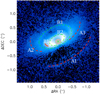 |
Fig. 2 Same image as Fig. 1a, but shown in logarithmic scale and overlaid with arcs and with the most prominent disk features highlighted. Two possible rings (R1 and R2, green dashed ellipses), three arcs (A1, A2 and A3, red dashed arc) and a small arc or blob in between the two rings (B1, red solid arc) are distinguished. While the red arcs only highlight the features mentioned above, the green dashed ellipses show the best fits for R1 and R2 with the fit parameters listed in Table 1. The gray circle at the location of the star shows the size of the coronagraph inner working angle. |
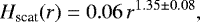
4.1 Ellipse fitting
To measure the offset of the ring-centers with respect to the star, we fit ellipses to R1 and R2 with the method discussed in de Boer et al. (2016). The ellipse-fit parameters are listed in Table 1. We note that the position angle (PA) along which the ellipses are offset with respect to the star (listed as “offset angle”, which increases from north to east) are within 7° from perpendicular to the PA of the ellipses, which is a prerequisite for the offset to be caused by the projection of the inclined circular rings that reside on a plane Hscat above the midplane. The offset of the inner ring R2 shifts its southwestern (near) side within the inner working angle of the coronograph, which makes the detection of signal at this part of the ring tentative. However, all other regions of this ring (e.g., the far side and along the major axis) are well outside this inner working angle. Therefore we confidently detected the inner edge or wall of the outer disk. We find that the inner wall lies at ~88 au, which is in remarkable agreement both with the inner disk radius of 82 au, as predicted byKhalafinejad et al. (2016) based on radiative transfer modeling of marginally resolved Q-band data, and with the inner edge of the submillimeter annulus detected at 75 au with ALMA by van der Plas et al. (2017). To determine the radial profile of the disk height Hscat (only possible to the first order because we consider the profile to be smooth and continuous and ignore the possible presence of gaps in the disk), we extrapolate the height at both rings to all radii by fitting a power law to the two data points as follows:
 (4)
(4)
with Hscat and r in au. This power law falls between the values that were recently determined for two ringed systems: the non-flaring disk (∝ r1) RX J1615.3-3255 (de Boer et al. 2016) and the strongly flaring (∝r1.73) HD 97048 (Ginski et al. 2016), and just above the average value (∝ r1.2) for five disks determined by Avenhaus et al. (2018).
It should be noted that the errors mentioned in Table 1 are merely the random errors for a fitting routine that only accepts an ellipse. However, a closer look at Fig. 2 shows that the outer ring R1 does not trace the fitted ellipse as well as R2. This deviation from a ring structure is best visible when we notice the asymmetry between the two ansae of the ellipse: locally more disk signal comes from regions just inside the green ellipse in the northwestern ansa, while on the southeastern ansa most of the signal is detected outside the fitted ellipse. When R1 is not a ring, the previously determined ellipse and flaring parameters are no longer valid. Therefore, we consider two scenarios as the extreme possibilities. In the first case, R1 is a ring (albeit irregularly shaped and/or illuminated) and the surface profile is strongly flared according to Eq. (4). In the second scenario, R1 is not a ring and we choose the flattest geometry that still allows R1 to be irradiated by the central star (i.e., no flaring), which is constrained by the height of R2, and written as
 (5)
(5)
4.2 Height-corrected deprojection
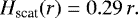
If we deproject the disk image to a face-on orientation, we can corroborate (or invalidate) that the disk is flaring according to Eq. (4) because this scenario should yield two concentric circles after deprojection. Height profiles, as given by Eqs. (4) and (5), allow us to determine Hscat(r) and subsequently determine for each pixel in the image a corresponding ellipse with offset u(r), using Eq. (3). We use these height maps to create a height-corrected deprojection, as illustrated in Fig. 3a for the non-flaring scenario. First, each pixel is shifted with − u(r), as found for the ellipse containing this pixel (Fig. 3b for the height map and Fig. 3e for the disk image). This process moves the surface features to the disk midplane (effectively creating a “thin disk” or flattened image), which yields the most appropriate image to compare with ALMA images of the midplane of the disk (van der Plas et al. 2017). For simplicity, we did not account for a signal originating from the bottom of the disk, such as feature A1, in which case these regions are shifted in the same direction (+ u) as their true offset. This moves the signal from the bottom side of the disk even further away from the center, which is convenient, as it avoids confusion between a signal originating from the top and the bottom. In the near- or forward-scattering side of the disk (southwest of the star, but very close to the inner cavity), we are strongly under-sampled: each new pixel on this side of the disk does not individually have a unique corresponding pixel in the original image. This point becomes clear when comparing the contours of the height maps in Figs. 3a, b: the contours in the southwestern side of the disk lie further apart in the flattened map (b) than in the height map of the original image (a). To account for this under-sampling, we resampled the original image with 3 × 3 subpixels and drew the pixel values for the thin disk image from pixels shifted by 3u in the original but resampled image. Figures 3c, f show the final step where we “stretch” or resample the flattened image along the minor axis by increasing the number of pixels in this direction with the factor 1∕cos(i), which produces the height-corrected deprojections for the height map and the disk image, respectively.
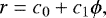
We investigated this height-corrected deprojection for two Hscat profiles: the non-flaring surface of Eq. (5) and the flaring surface of Eq. (4) in Fig. 4 in panels a and b, respectively. The southwest (PA ~ 230°) of panel b isplagued by the fact that the value for multiple pixels are drawn from the same point in the original image because the height profile of the near side of the inclined power law creates a stronger under-sampling than for the non-flared profile. The green dashed line shows a circle with a radius equal to the semimajor axis of R2 from Table 1, which traces the local maxima on the disk surface brightness just outside the cavity in both panels.This inner rim does not show a ring with a homogeneous brightness distribution for each azimuth angle. In Appendix A, we show that we expect such asymmetries for this ring even when it is illuminated homogeneously owing to variations in the scattering phase function with azimuth angle. The orange dashed line in Figs. 4a, b shows a circle with the radius based on the semimajor axis of R1 from Table 1. As expected for the non-flared height correction of Fig. 4a, where R1 is not assumed to be a ring, the orange circle does not trace the outer disk feature very well. Roughly between − 45° ≤PA ≤ 45°, the orange circle coincides with the local maxima in the disk, while for 45° ≤PA ≤ 135° and 225° ≤PA ≤ 315° the local maxima lie outside and inside of the orange circle, respectively. For the remaining PAs in the south it is rather difficult to associate and compare any local maxima with the circle shape. In panel b of Fig. 4, in which we make the assumption that R1 is a ring, the local maxima lie closer to the orange circle. However, we can discern a similar trend of the local maxima lying inside the orange circle in the western side and outside of this circle on the east, albeit much more subtle than for panel a. Based on the deprojections for the two extreme height profiles, we conclude that the outer disk is most likely not shaped like a ring.
4.3 Single-armed spiral
The deviation of the outer disk feature from a circular shape, as shown in Fig. 4, shows a general trend (i.e., moving outward in counter-clockwise direction) that is consistent between the two extreme possibilities for the height profile. Although we cannot fully dismiss that the outer region is circular in panel b, it is more likely that the structure behaves according to a spiral pattern.
In Fig. 5b, we overlay a simple (single-armed) Archimedean spiral (outer green-white-orange dashed line) on the deprojection using the non-flaring height profile. The spiral can be described by
 (6)
(6)
where ϕ is the azimuth angle in degrees, c0 ~ 180 au and c1 ~ 0.2 au degree−1. For r ≳ 200 au this spiral traces the local maxima better than the orange dashed circle in Figs. 4a, b. The green dashed line traces the brightest regions and winds outward in a counter-clockwise direction from a PA of ~ 270° for another 270°. The white dashed lines show parts where the signal-to-noise ratio is too low to determine the local maxima, but are shown to illustrate that the outer and inner arms can be described with only two connected, yet distinct spiral patterns.
The orange dashed line (PA ~ 90°) reconnects the spiral to the local maxima of feature A2. The spiral opening angle of ~ 0.2 au degree−1 should be considered to be an upper limit because the outer disk structure more closely resembles a circular ring when we use the r1.35 height profile for the deprojection, as we discussed at the end of Sect. 4.2. Hydrodynamical modeling of disks perturbed by embedded companions often show single-armed spirals both inside and outside the orbital radius (rc) of the companion. The spiral opening angles in the model disks outside rc either remain constant for a large range r (Ogilvie & Lubow 2002; Ragusa et al. 2017) or opening angles decreasing with r (Dong et al. 2015).
For r < rc, the aforementioned models all predict spiral opening angles that are larger than outside rc. The under-sampling in the south–southwestern region does not allow us to determine confidently how the pattern winds inward from the innermost point of the green dashed line. However, we detect a sudden increase in the spiral opening angle at PA ~ 270°, r ~200 au (transition from green-dashed into red-dashed line). This change in spiral opening angle allows for the option in which the feature B1 in the southeast is connected to the spiral pattern of the outer disk through a more complex spiral pattern with radially varying opening angle. Feature A3 is much more diffuse after the deprojection, but it does not seem possible to be explained with the simple spiral of Eq. (6).
 |
Fig. 3 (a): map of the height profile using the function H scat (r) = 0.29r. (b): height map shifted with Hscat × sin i in the direction of the minor axis to create concentric ellipses. (c): the centered height map of panel b is stretched along the minor axis with 1∕ cos i. (d): original inclination corrected r2 scaled Qphi image (as Fig. 1)c. (e): ophi image shifted in the same way as the height map in panel b. This step creates a “flattened” but inclined image. (f): stretched following the deprojection of panel c, to show the disk similar to a face-on orientation. |
 |
Fig. 4 (a): height-corrected deprojection using the non-flaring height profile (Eq. (5)). This deprojection is the same as for Fig. 3f, but is shown in log scale (not r2 scaled). (b): as panel a, but deprojected with the flaring height profile (Eq. (4)). |
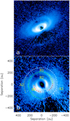 |
Fig. 5 (a): for comparison, the log-scaled Qphi image is shown again without highlighted features. The tick marks are the same as for Fig. 2. (b): spiral arm overlayed on the deprojected image (log scale) using the non-flaring height profile, with the same feature annotations as used in Fig. 2. The outer green-white-orange spiral (containing features R1 and A2) is a simple Archimedean spiral as described by Eq. (6), while the inner red-white-red dashed line is a mere illustration of how B1 could be connected to the base of the green spiral. The green and orange dashed lines trace the R1 and A2 structures, respectively. The red dashed lines, which trace the inner structures to the southeast and southwest of the star, clearly have different spiral properties than the outer spiral, most notably at the transition from red to green. Although no clear radial peak is detected at the positions of the white dashed lines in both the outer and inner structures, they follow the same behavior as the outer and the inner arms, respectively. Feature A3 is difficult to recognize because it is stretched into a diffuse region outside the white spiral and is not described by any dashed line. |
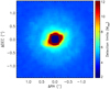 |
Fig. 6 Detection map of ADI result in the H2 filter expressed in Jupiter masses based on the DUSTY models (Chabrier et al. 2000). The region containing disk signal contains ~ 3–4 times higher upper limits than the background owing to noise added to the post-processing routine by the disk signal. |
4.4 Planet detection limits
Figure 6 shows a map of the detection limits in the H2 filter based on an angular differential imaging (ADI; Marois et al. 2006)reduction of the SHINE data. The mass limits are based on the DUSTY models (Chabrier et al. 2000). At large separations r ≳ 1′′, we reach an upper limit of ~ 5MJup. However, the ADI routine is strongly affected by the large azimuthal asymmetries in the disk, which dominates the noise at smaller separations. Furthermore, if a planet orbits the star at these smaller separations near the disk midplane, its thermal emission is heavily extincted as a result of scattering and absorption of the surrounding circumstellar disk. Therefore, we cannot conclude from these observations that there is no companion of mass higher than shown in Fig. 6 orbiting within 1′′ from the star. However, because neither our SPHERE polarimetric images nor the ALMA continuum images of van der Plas et al. (2017) reveal any signal from the dust disk at r ≳ 1′′, we consider the ~ 5MJup limit at larger separations to be reliable.
5 Discussion
5.1 Single-armed spiral pattern in the outer disk
For disks for which it is possible to determine a first-order estimate of the height profile, the height-corrected deprojection we present in Sect. 4.2 offers a useful tool to both further constrain the shape of the height profile and to analyze whether disk features are circular or deviate from this shape. Although it cannot fully be ruled out that feature R1 is a circular ring, Figs. 4 and 5b show that a single-armed spiral nature of this feature is more plausible.
Spiral density waves in the gas are a common prediction of hydrodynamic models of planet–disk interaction. Typically multiple spiral arms are excited inside of the planet location, while outside of the planet location single-armed spirals are possible (Zhu et al. 2015; Dong et al. 2015; Fung & Dong 2015; Dong & Fung 2017; Miranda & Rafikov 2019). If we assume that the spiral structure seen in HD 34282 is caused by a single planet then this leaves us with two main scenarios. In the first scenario, the planet is located close to the northern tip of feature B1, that is, the structure we trace is entirely located outside of the planetary orbit. In the second case, the planet is located further out, but the resulting spiral arms are too tightly wound to be resolved in the SPHERE observations.
The first scenario would make the feature that we trace in the outer disk a “true” single-armed spiral. The shape and contrast of spiral features depends on the precise parameters of the disk and the perturber. Dong et al. (2015) showed that inner and outer spiral features vary significantly based on the mass of the pertuber, its location in the disk, and the thermal properties of the disk; that is, they investigated the extreme isothermal and adiabatic cases. For higher planet masses (6 MJup) in the latter work, the outer arm in the disk is typically not clearly visible. This is similar to later results in Dong et al. (2016), where it is shown that a low-mass stellar companion does not excite detectable outer arms. Similarly, companions at smaller separations to the primary star drive more prominent outer spiral arms (Dong et al. 2015). However, across different models the inner spiral arms are typically significantly brighter than the outer spiral arm. This is not very consistent with our data since we presumably would predict the outer spiral but not the inner spirals. Nonetheless, it is possible that the perturbing planet is located close to the inner disk in the case of HD 34282, which is consistent with a prominent outer spiral arm. In that case, it may be that we lack the resolution and sensitivity to pick up the inner arms close to the coronagraphic mask.
In the second scenario, the planet may be located anywhere along the spiral feature in principle. One plausible location would be the discontinuity between the innermost part of the feature we trace from the southeast to the southwest and the outer part of the structure, as discussed in Sect. 4.3; the connection point of the red-white dashed line and the green-dashed line in Fig. 5b. The discontinuity might indicate the “shoulder” typically visible at the planet location in hydrodynamic simulations. This scenario is similar to that shown in Dong et al. (2016) for a 3 MJup planet under a 50° inclination and a PA of 150° (see their Fig. A.1). We note however that we do not see a clear connection of feature B1 to the northeastern part of the disk, as is visible in the Dong et al. models. Such a placement of the planet would, in any case, make the bright feature B1 and its continuation, denoted with a red-dashed line in Fig. 5b, inner spiral structures. The remaining (fainter) structures that are traced in 5b would then be part of an outer spiral arm. This brightness distribution is consistent with the discussed models.
In either scenario, we have to take into account that lower planet masses typically produce more tightly wound spirals (see, e.g., Dong et al. 2015). Thus, the lower the planet mass, the harder a single-armed spiral is distinguishable from multiarmed spirals. Thisis consistent with the SPHERE detection limits shown in Fig. 6, which give a tentative upper limit of 6–7 MJup at the suspected planet locations (with the caveats mentioned in Sect. 4.4).
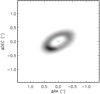 |
Fig. 7 ALMA band 7 continuum image (van der Plas et al. 2017). The disk is detected in as an annulus, with an azimuthal asymmetry at PA=135. Contrary to the SPHERE detection of the scattering surface, the submillimeter image probes the midplane of the disk. Therefore, the annulus detected with ALMA does not show a height-induced offset, but is centered around the star. |
5.2 Comparison with ALMA continuum image
The ALMA data of van der Plas et al. (2017) (Fig. 7) do not display a spiral pattern, rather they reveal a single broadannulus with an inner cavity consistent with our observations. The otherwise smooth annulus in the continuum image does display an increase in surface brightness at a similar radius and (slightly larger) PA as our B1 feature. This approximate overlap between the NIR and submillimeter asymmetric features supports the scenarios suggested by van der Plas et al.: we either detected a local increase in temperature or we are seeing a horseshoe,induced by either a vortex or an over-density in the gas disk (Ragusa et al. 2017), similar to the horse-shoe features detected in the disks of MWC 147 (van der Marel et al. 2013) and HD 142527 (Casassus et al. 2013).
Recent modeling work by Dong et al. (2017) shows the simulated H-band images of a disk containing a super-earth that display a faint trace of a single-armed spiral pattern (although the detectability is questioned by the authors), while the simulated submillimeter images are not sensitive to the spiral pattern and only show a gap. Long baseline ALMA observations of HD 34282 are required to definitively determine whether there is a spiral pattern and/or a gap in the submillimeter dust; this gap is located outside the inner rim of the disk, possibly coincident with the dark region we detect at ~ 150 au. We leave the detailed analysis of the spiral pattern and the possibility of deriving properties of a potential protoplanet for future work,in which we will examine ALMA continuum images and these SPHERE data with radiative transfer modeling.
6 Conclusions
The first detection of the protoplanetary disk around HD 34282 in scattered light reveals a disk surface rich in structure. In accordance with the model predictions of Khalafinejad et al. (2016), the disk contains a cavity surrounded by the puffed-up inner rim of the disk at 88 au. Because of the inclination (i =56°) of the system, the disk displays indications of its large vertical extent: the top side of the disk appears offset from the star center, while the bottom side is clearly visible with an opposing offset.
We create two surface height profiles: one using a constant Hscat∕r = 0.29 and the other using a power law ∝ r1.35. Both profiles are used to perform a height-corrected deprojection or “rotation” of the disk to simulate face-on images of the disk. This deprojection shows evidence that the disk region outside the puffed- up inner rim (R2) contains a tightly wound single-armed spiral, winding outward in counter-clockwise direction. Although the outermost region can be approximated by the Archimedean spiral description of Eq. (6), the region inward of r ~ 180 au cannot be described in such simple terms.
In future work, we will continue investigating HD 34282 system by performing radiative transfer modeling including both the ALMA data of van der Plas et al. (2017) and the presented SPHERE data. Subsequently, we will observe the disk with ALMA with a longer baseline to obtain submillimeter images of a resolution comparable to that of our SPHERE observations, to search for substructure in the annulus detected by van der Plas et al. (2017).
Acknowledgements
We thank Ruobing Dong for our discussions on the appearance of inclined spiral systems. J.dB. acknowledges the funding by the European Research Council under ERC Starting Grant agreement 678194 (FALCONER). SPHERE is an instrument designed and built by a consortium consisting of IPAG (Grenoble, France), MPIA (Heidelberg, Germany), LAM (Marseille, France), LESIA (Paris, France), Laboratoire Lagrange (Nice, France), INAF - Osservatorio di Padova (Italy), Observatoire de Genève (Switzerland), ETH Zurich (Switzerland), NOVA (The Netherlands), ONERA (France), and ASTRON (The Netherlands) in collaboration with ESO. SPHERE was funded by ESO, with additional contributions from CNRS (France), MPIA (Germany), INAF (Italy), FINES (Switzerland), and NOVA (The Netherlands). SPHERE also received funding from the European Commission Sixth and Seventh Framework Programmes as part of the Optical Infrared Coordination Network for Astronomy (OPTICON) under grant number RII3-Ct2004-001566 for FP6 (2004–2008), grant number 226604 for FP7 (2009–2012), and grant number 312430 for FP7 (2013–2016).
Appendix A Phase-function variations
The resulting height-corrected deprojections, shown in Fig. 4a and b simulate the rotation of the disk toward a face-on (i =0°) orientation. The main difference with a truly face-on observation of the disk is that the large azimuthal variation of the scattering angles (always ~90° for a truly face-on disk) are not corrected for. While a homogeneous ring centered around the star would not vary in surface brightness for a truly face-on disk, it does still vary in the azimuthal direction after our height-corrected deprojection as a result of variations in the scattering phase function. To illustrate this effect, we created a simple disk ring seen at i = 56° (Fig. A.1a) with the radiative transfer code MCFOST (Pinte et al. 2006). Subsequently, after setting the central eight pixels to zero to mimic the presence of a coronagraph mask, we rotated the image using the same height-corrected deprojectionas used in Fig. 3. Finally, we smoothed the image with a Gaussian of full width at half maximum of three pixels.This deprojected model image, shown in Fig. A.1b, shows similar variations in surface brightness along the ring: bright at small (forward) scattering angles and faint for large (backward) scattering angles.
Furthermore, it is important to note the effect of the deprojection on the bottom side of the ring. The shift to reverse the offset u of the scattering surface (as shown in the second column of Fig. 3) is only performed in one direction: toward the southwest. However, the bottom side of the disk has an offset in the direction opposite to the top surface and is therefore shifted in the wrong direction (even further away from the star center). Although the bottom of ring R2 is not detected for HD 34282, feature A1 most likely represents the bottom of the outer regions (R1 or even further out) of the disk and is therefore shifted too far away from the center in our deprojection as well (outside the frame of Fig. 3f). However, the aim of the height-corrected deprojection is to simulate a face-on orientation, at which it would be completely impossible to see the bottom side (for an optically thick disk). Since the signal from the bottom regions (A1) of the disk is shifted away from the top surface we avoided contamination of the top surface.
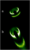 |
Fig. A.1 (a): radiative transfer (MCFOST) disk-model comprised of a single ring with similar i and H scat /r as the disk of HD 34282. A software mask is added to the star center of the image to simulate the presence of a coronagraph mask. Finally the image is smoothed with a Gaussian. (b): the model image of panel a after a height-corrected deprojection. This method shifts the bottom side of the disk (arc in bottom-right corner of the image) in the wrong direction. |
References
- Alexander, R. D., Clarke, C. J., & Pringle, J. E. 2006, MNRAS, 369, 216 [Google Scholar]
- ALMA Partnership (Brogan, C. L., et al.) 2015, ApJ, 808, L3 [NASA ADS] [CrossRef] [Google Scholar]
- Avenhaus, H., Quanz, S. P., Garufi, A., et al. 2018, ApJ, 863, 44 [Google Scholar]
- Benisty, M., Stolker, T., Pohl, A., et al. 2017, A&A, 597, A42 [NASA ADS] [CrossRef] [EDP Sciences] [Google Scholar]
- Beuzit, J. L., Vigan, A., Mouillet, D., et al. 2019, A&A, 631, A155 [NASA ADS] [CrossRef] [EDP Sciences] [Google Scholar]
- Boccaletti, A., Abe, L., Baudrand, J., et al. 2008, in SPIE Conf. Ser., 7015, Adaptive Optics Systems, 70151B [Google Scholar]
- Canovas, H., Perez, S., Dougados, C., et al. 2015, A&A, 578, A1 [NASA ADS] [CrossRef] [EDP Sciences] [Google Scholar]
- Casassus, S., van der Plas, G., M, S. P., et al. 2013, Nature, 493, 191 [NASA ADS] [CrossRef] [Google Scholar]
- Chabrier, G., Baraffe, I., Allard, F., & Hauschildt, P. 2000, ApJ, 542, 464 [Google Scholar]
- Claudi, R. U., Turatto, M., Gratton, R. G., et al. 2008, in SPIE Conf. Ser., 7014, Ground-based and Airborne Instrumentation for Astronomy II, 70143E [Google Scholar]
- Cuello, N., Louvet, F., Mentiplay, D., et al. 2020, MNRAS, 491, 504 [Google Scholar]
- de Boer, J., Salter, G., Benisty, M., et al. 2016, A&A, 595, A114 [NASA ADS] [CrossRef] [EDP Sciences] [Google Scholar]
- de Boer, J., Langlois, M., van Holstein, R. G., et al. 2020, A&A, 633, A63 [NASA ADS] [CrossRef] [EDP Sciences] [Google Scholar]
- de Juan Ovelar, M., Min, M., Dominik, C., et al. 2013, A&A, 560, A111 [NASA ADS] [CrossRef] [EDP Sciences] [Google Scholar]
- Dipierro, G., Pinilla, P., Lodato, G., & Testi, L. 2015, MNRAS, 451, 974 [Google Scholar]
- Dohlen, K., Langlois, M., Saisse, M., et al. 2008, in SPIE Conf. Ser., 7014, The Infra-red Dual Imaging and Spectrograph for SPHERE: Design and Performance, 70143L [Google Scholar]
- Dong, R., & Fung, J. 2017, ApJ, 835, 38 [NASA ADS] [CrossRef] [Google Scholar]
- Dong, R., Zhu, Z., Rafikov, R. R., & Stone, J. M. 2015, ApJ, 809, L5 [Google Scholar]
- Dong, R., Fung, J., & Chiang, E. 2016, ApJ, 826, 75 [NASA ADS] [CrossRef] [Google Scholar]
- Dong, R., Li, S., Chiang, E., & Li, H. 2017, ApJ, 843, 127 [NASA ADS] [CrossRef] [Google Scholar]
- Flock, M., Ruge, J. P., Dzyurkevich, N., et al. 2015, A&A, 574, A68 [NASA ADS] [CrossRef] [EDP Sciences] [Google Scholar]
- Fung, J., & Dong, R. 2015, ApJ, 815, A21 [Google Scholar]
- Gaia Collaboration (Brown, A. G. A., et al.) 2018, A&A, 616, A1 [NASA ADS] [CrossRef] [EDP Sciences] [Google Scholar]
- Ginski, C., Stolker, T., Pinilla, P., et al. 2016, A&A, 595, A112 [NASA ADS] [CrossRef] [EDP Sciences] [Google Scholar]
- Grady, C. A., Muto, T., Hashimoto, J., et al. 2013, ApJ, 762, 48 [Google Scholar]
- Greaves, J. S., Mannings, V., & Holland, W. S. 2000, Icarus, 143, 155 [NASA ADS] [CrossRef] [Google Scholar]
- Khalafinejad, S., Maaskant, K. M., Mariñas, N., & Tielens, A. G. G. M. 2016, A&A, 587, A62 [NASA ADS] [CrossRef] [EDP Sciences] [Google Scholar]
- Lagage, P.-O., Doucet, C., Pantin, E., et al. 2006, Science, 314, 621 [NASA ADS] [CrossRef] [PubMed] [Google Scholar]
- Langlois, M., Dohlen, K., Vigan, A., et al. 2014, in Society of Photo-Optical Instrumentation Engineers (SPIE) Conference Series, 9147, Ground-based and Airborne Instrumentation for Astronomy V, 91471R [Google Scholar]
- Lodato, G., & Rice, W. K. M. 2004, MNRAS, 351, 630 [Google Scholar]
- Maaskant, K. M., Min, M., Waters, L. B. F. M., & Tielens, A. G. G. M. 2014, A&A, 563, A78 [NASA ADS] [CrossRef] [EDP Sciences] [Google Scholar]
- Macintosh, B., Graham, J. R., Ingraham, P., et al. 2014, ArXiv e-prints [arXiv:1403.7520] [Google Scholar]
- Maire, A.-L., Langlois, M., Dohlen, K., et al. 2016, in SPIE Conf. Ser., 9908, Ground-based and Airborne Instrumentation for Astronomy VI, 990834 [Google Scholar]
- Marois, C., Lafrenière, D., Doyon, R., Macintosh, B., & Nadeau, D. 2006, ApJ, 641, 556 [Google Scholar]
- Martinez, P., Dorrer, C., Aller Carpentier, E., et al. 2009, A&A, 495, 363 [NASA ADS] [CrossRef] [EDP Sciences] [Google Scholar]
- Ménard, F., Cuello, N., Ginski, C., et al. 2020, A&A, 639, A1 [CrossRef] [Google Scholar]
- Merín, B., Montesinos, B., Eiroa, C., et al. 2004, A&A, 419, 301 [NASA ADS] [CrossRef] [EDP Sciences] [Google Scholar]
- Miranda, R., & Rafikov, R. R. 2019, ApJ, 875, 37 [Google Scholar]
- Montesinos, M., Perez, S., Casassus, S., et al. 2016, ApJ, 823, L8 [NASA ADS] [CrossRef] [Google Scholar]
- Muto, T., Grady, C. A., Hashimoto, J., et al. 2012, ApJ, 748, L22 [NASA ADS] [CrossRef] [Google Scholar]
- Ogilvie, G. I., & Lubow, S. H. 2002, MNRAS, 330, 950 [NASA ADS] [CrossRef] [Google Scholar]
- Ohta, Y., Fukagawa, M., Sitko, M. L., et al. 2016, PASJ, 68, 53 [NASA ADS] [CrossRef] [Google Scholar]
- Piétu, V., Dutrey, A., & Kahane, C. 2003, A&A, 398, 565 [NASA ADS] [CrossRef] [EDP Sciences] [Google Scholar]
- Pinilla, P., Flock, M., Ovelar, M. d. J., & Birnstiel, T. 2016, A&A, 596, A81 [NASA ADS] [CrossRef] [EDP Sciences] [Google Scholar]
- Pinte, C., Ménard, F., Duchêne, G., & Bastien, P. 2006, A&A, 459, 797 [NASA ADS] [CrossRef] [EDP Sciences] [Google Scholar]
- Quanz, S. P., Avenhaus, H., Buenzli, E., et al. 2013, ApJ, 766, L2 [NASA ADS] [CrossRef] [Google Scholar]
- Ragusa, E., Dipierro, G., Lodato, G., Laibe, G., & Price, D. J. 2017, MNRAS, 464, 1449 [NASA ADS] [CrossRef] [Google Scholar]
- Schmid, H. M., Joos, F., & Tschan, D. 2006, A&A, 452, 657 [NASA ADS] [CrossRef] [EDP Sciences] [Google Scholar]
- Sylvester, R. J., Skinner, C. J., Barlow, M. J., & Mannings, V. 1996, MNRAS, 279, 915 [NASA ADS] [CrossRef] [Google Scholar]
- van Boekel, R., Henning, T., Menu, J., et al. 2017, ApJ, 837, 132 [NASA ADS] [CrossRef] [Google Scholar]
- van der Marel,N., van Dishoeck, E. F., Bruderer, S., et al. 2013, Science, 340, 1199 [NASA ADS] [CrossRef] [PubMed] [Google Scholar]
- van der Plas, G., Ménard, F., Canovas, H., et al. 2017, A&A, 607, A55 [NASA ADS] [CrossRef] [EDP Sciences] [Google Scholar]
- van Holstein, R. G., Girard, J. H., de Boer, J., et al. 2020, A&A, 633, A64 [NASA ADS] [CrossRef] [EDP Sciences] [Google Scholar]
- Vigan, A., Moutou, C., Langlois, M., et al. 2010, MNRAS, 407, 71 [NASA ADS] [CrossRef] [Google Scholar]
- Vioque, M., Oudmaijer, R. D., Baines, D., Mendigutía, I., & Pérez-Martínez, R. 2018, A&A, 620, A128 [NASA ADS] [CrossRef] [EDP Sciences] [Google Scholar]
- Zhu, Z., Dong, R., Stone, J. M., & Rafikov, R. R. 2015, ApJ, 813, 88 [NASA ADS] [CrossRef] [Google Scholar]
An exception may be the disk around V1247 Ori observed by Ohta et al. (2016), who mention the possibility of a single spiral arm based on their data.
With the notable exception of stellar fly-by induced structures, see, e.g., Cuello et al. (2020); Ménard et al. (2020).
All Tables
All Figures
|
Fig. 1 Polarimetric images of HD 34282 by VLT/SPHERE/IRDIS. In all panels, north is up, east is left, and the star center is annotated with a green cross. All images are shown on a linear color map. (a) The Qϕ image showsthe inner cavity, surrounded by the bright inner edge (or wall) of the outer disk as an ellipse with its center slightly offset from the star in the northeastern direction. Faint structures are detected directly outside this inner wall. (b) The Uϕ image shownwith the same intensity range as panel a. (c) To highlight the outer disk structures we scaled the Qϕ image with the disk radius squared, corrected for the inclination (Piétu et al. 2003, 56°). To a first order, this r2 scaling accounts for the decrease in stellar irradiation of the disk. The height of the scattering surface was not taken into account, thus this scaling is only shown for illustrative purpose so as to highlight the fainter structures outside the inner wall. (d) Uϕ with the same r2 scaling and shown for the same intensity range as panel c. |
| In the text | |
|
Fig. 2 Same image as Fig. 1a, but shown in logarithmic scale and overlaid with arcs and with the most prominent disk features highlighted. Two possible rings (R1 and R2, green dashed ellipses), three arcs (A1, A2 and A3, red dashed arc) and a small arc or blob in between the two rings (B1, red solid arc) are distinguished. While the red arcs only highlight the features mentioned above, the green dashed ellipses show the best fits for R1 and R2 with the fit parameters listed in Table 1. The gray circle at the location of the star shows the size of the coronagraph inner working angle. |
| In the text | |
|
Fig. 3 (a): map of the height profile using the function H scat (r) = 0.29r. (b): height map shifted with Hscat × sin i in the direction of the minor axis to create concentric ellipses. (c): the centered height map of panel b is stretched along the minor axis with 1∕ cos i. (d): original inclination corrected r2 scaled Qphi image (as Fig. 1)c. (e): ophi image shifted in the same way as the height map in panel b. This step creates a “flattened” but inclined image. (f): stretched following the deprojection of panel c, to show the disk similar to a face-on orientation. |
| In the text | |
|
Fig. 4 (a): height-corrected deprojection using the non-flaring height profile (Eq. (5)). This deprojection is the same as for Fig. 3f, but is shown in log scale (not r2 scaled). (b): as panel a, but deprojected with the flaring height profile (Eq. (4)). |
| In the text | |
|
Fig. 5 (a): for comparison, the log-scaled Qphi image is shown again without highlighted features. The tick marks are the same as for Fig. 2. (b): spiral arm overlayed on the deprojected image (log scale) using the non-flaring height profile, with the same feature annotations as used in Fig. 2. The outer green-white-orange spiral (containing features R1 and A2) is a simple Archimedean spiral as described by Eq. (6), while the inner red-white-red dashed line is a mere illustration of how B1 could be connected to the base of the green spiral. The green and orange dashed lines trace the R1 and A2 structures, respectively. The red dashed lines, which trace the inner structures to the southeast and southwest of the star, clearly have different spiral properties than the outer spiral, most notably at the transition from red to green. Although no clear radial peak is detected at the positions of the white dashed lines in both the outer and inner structures, they follow the same behavior as the outer and the inner arms, respectively. Feature A3 is difficult to recognize because it is stretched into a diffuse region outside the white spiral and is not described by any dashed line. |
| In the text | |
|
Fig. 6 Detection map of ADI result in the H2 filter expressed in Jupiter masses based on the DUSTY models (Chabrier et al. 2000). The region containing disk signal contains ~ 3–4 times higher upper limits than the background owing to noise added to the post-processing routine by the disk signal. |
| In the text | |
|
Fig. 7 ALMA band 7 continuum image (van der Plas et al. 2017). The disk is detected in as an annulus, with an azimuthal asymmetry at PA=135. Contrary to the SPHERE detection of the scattering surface, the submillimeter image probes the midplane of the disk. Therefore, the annulus detected with ALMA does not show a height-induced offset, but is centered around the star. |
| In the text | |
|
Fig. A.1 (a): radiative transfer (MCFOST) disk-model comprised of a single ring with similar i and H scat /r as the disk of HD 34282. A software mask is added to the star center of the image to simulate the presence of a coronagraph mask. Finally the image is smoothed with a Gaussian. (b): the model image of panel a after a height-corrected deprojection. This method shifts the bottom side of the disk (arc in bottom-right corner of the image) in the wrong direction. |
| In the text | |
Current usage metrics show cumulative count of Article Views (full-text article views including HTML views, PDF and ePub downloads, according to the available data) and Abstracts Views on Vision4Press platform.
Data correspond to usage on the plateform after 2015. The current usage metrics is available 48-96 hours after online publication and is updated daily on week days.
Initial download of the metrics may take a while.