| Issue |
A&A
Volume 633, January 2020
|
|
|---|---|---|
| Article Number | A159 | |
| Number of page(s) | 13 | |
| Section | Extragalactic astronomy | |
| DOI | https://doi.org/10.1051/0004-6361/201935782 | |
| Published online | 27 January 2020 | |
Bright Lyman-α emitters among Spitzer SMUVS galaxies in the MUSE/COSMOS field⋆
1
Kapteyn Astronomical Institute, University of Groningen, PO Box 800, 9700 Groningen, The Netherlands
e-mail: rosani@astro.rug.nl
2
Cosmic Dawn Center (DAWN), Niels Bohr Institute, University of Copenhagen, Juliane Maries vej 30, 2100 Copenhagen, Denmark
Received:
26
April
2019
Accepted:
12
November
2019
We search for the presence of bright Lyα emitters among Spitzer SMUVS galaxies at z > 2.9 making use of homogeneous MUSE spectroscopic data. Although these data only cover a small region of COSMOS, MUSE has the unique advantage of providing spectral information over the entire field, without the need of target pre-selection. This results in an unbiased detection of all the brightest Lyα emitters among the SMUVS sources, which by design are stellar-mass selected galaxies. Within the studied area, ∼14% of the SMUVS galaxies at z > 2.9 have Lyα fluxes Fλ ≳ 7 × 10⁻¹⁸ erg s−1 cm−2. These Lyα emitters are characterized by three types of emission, 47% show a single-line profile, 19% present a double peak or a blue bump, and 31% show a red tail. One object (3%) shows both a blue bump and a red tail. We also investigate the spectral energy distribution (SED) properties of the SMUVS galaxies that are MUSE detected and those that are not. After stellar mass matching the two populations, we find that the MUSE detected galaxies have generally lower extinction than SMUVS-only objects, while there is no clear intrinsic difference in the mass and age distributions of the two samples. For the MUSE-detected SMUVS galaxies, we compare the instantaneous star formation rate lower limit obtained from the Lyα line with its past average derived from SED fitting, and find evidence for rejuvenation in some of our oldest objects. In addition, we study the spectra of those Lyα emitters that are not detected in SMUVS in the same field. We find that of the emission line profiles shown 67% have a single line, 3% a blue bump, and 30% a red tail. The difference in profile distribution could be ascribed to the fainter Lyα luminosities of the MUSE sources not detected in SMUVS and an intrinsically different mass distribution. Finally, we search for the presence of galaxy associations using the spectral redshifts. The integral coverage of MUSE reveals that these associations are 20 times more likely than what is derived from all the other existing spectral data in COSMOS, which is biased by target pre-selection.
Key words: galaxies: high-redshift / galaxies: star formation / cosmology: observations
Full Table A.1 is only available at the CDS via anonymous ftp to cdsarc.u-strasbg.fr (130.79.128.5) or via http://cdsarc.u-strasbg.fr/viz-bin/cat/J/A+A/633/A159
© ESO 2020
1. Introduction
The Lyman-α (Lyα) line contains important information about some of the main physical processes occurring in galaxies. In particular, bright Lyα emitters are tracers of the most prominent unobscured star formation activity at different cosmic times. The interpretation of the Lyα line is not trivial, however, because of its resonant nature; it is easily scattered by the interstellar medium (ISM) on its way out of the galaxy. Furthermore, Lyα photons are absorbed by dust and re-emitted at longer wavelengths, thus subtracting them from the line intensity. The kinematics of the gas also needs to be taken into account. All these processes give rise to different line profile shapes depending on the conditions surrounding the emitter galaxy (Shapley et al. 2003; Karman et al. 2014, 2017; Martin et al. 2015; Dijkstra 2017; Hernán-Caballero et al. 2017; Bridge et al. 2018; Erb et al. 2018; Gurung-Lopez et al. 2019; Nakajima et al. 2018; Orlitová et al. 2018; Sobral et al. 2018; Vanzella et al. 2018; Kimm et al. 2019; Marchi et al. 2019; Remolina-Gutiérrez & Forero-Romero 2019; Smith et al. 2019).
It is possible to recover the original Lyα flux if information on the Hα line is available. There is no canonical conversion factor between Lyα and Hα because secondary effects influence the conversion, but assuming case B recombination the values can reasonably range from ≈8 (Dijkstra 2017) to ∼8.7 (Hu et al. 1998). When information on the Hα line is not present, we can rely on radiative transfer models exclusively treating the Lyα line to try and recover the original emission from line shape fitting. These models need to take into account the composition of the circumgalactic medium, the presence of dust, how dense the neutral hydrogen is, as well as the gas dynamics and the time evolution of the medium along with the star formation event. Models reproducing the shape of the Lyα emission go from the early approach of Tenorio-Tagle et al. (1999) and Mas-Hesse et al. (2003) to the more recent models by Verhamme et al. (2008, 2018), Gronke (2017), and Kakiichi & Gronke (2019), among others. Finally, selecting objects using the Lyα line is a way to ensure that the more active star-forming non-dusty galaxies are selected (Zhang et al. 2019).
The use of Spitzer (Werner et al. 2004) data in the 3.6/4.5 μm bands allows us to access the red flat part of the spectrum of high-redshift galaxies. This results in a stellar mass selection, as the more luminous high-z galaxies at those wavelengths are typically the most massive. These objects are interesting because they represent possible progenitors of today’s most massive galaxies and because they possibly played an integral role in the peak of star formation history around z ∼ 2 (Caputi et al. 2011; Deshmukh et al. 2018; Martinache et al. 2018).
By combining the more massive galaxies selected by Spitzer and the most prominent Lyα emitters, we probe a very specific part of the galaxy evolution picture. We not only select the most massive objects at early times, but we also ensure that they are intensely star-forming and contain relatively little dust by detecting their Lyα emission.
Previous studies combining Lyα information with photometric SED fitting have been able to constrain stellar mass, age, star formation rate (SFR), and E(B − V) of Lyα emitters among other properties. The general result of these studies is that Lyα emitters are young, prominently star-forming, mostly unobscured intermediate-mass galaxies. Some of these studies also find evidence of more massive objects being present among the Lyα population. Moreover, the age distribution of the Lyα emitters presents in some cases an age bimodality, for which a significant fraction of the galaxies studied is not young, but has ages around 1 Gyr (Lai et al. 2008; Finkelstein et al. 2009; Ono et al. 2010; Pentericci et al. 2009, 2010; Yuma et al. 2010; Guaita et al. 2011; Acquaviva et al. 2012; Mallery et al. 2012; Curtis-Lake et al. 2013; McLinden et al. 2014; De Barros et al. 2017; Hao et al. 2018; Marchi et al. 2019).
Among the best studied blank areas of the sky is the COSMOS field (Scoville et al. 2007), for which a wide range of homogeneous and deep data sets are available. One of the surveys spanning part of the field is the Spitzer Matching Survey of the UltraVISTA ultra-deep Stripes (SMUVS, Ashby et al. 2018). The SMUVS survey combines Spitzer 3.6 and 4.5 μm data with 26 complementary photometric bands to infer the redshift and physical properties of its galaxies. Most importantly, it uses the Spitzer InfraRed Array Camera (IRAC) data (Fazio et al. 2004) to gain access to the flat part of the continuum of high-redshift objects. The SMUVS survey has already produced a number of studies of galaxy properties at redshift z > 2 (Caputi et al. 2017; Cowley et al. 2018, 2019; Deshmukh et al. 2018).
The Multi Unit Spectroscopic Explorer spectrograph (MUSE, Bacon et al. 2010) provides a powerful tool to expand the existing analysis of any part of the sky. Being an integral field unit (IFU) spectrograph, it allows to take the spectra of a ∼1′×1′ portion of the sky with no source pre-selection. Furthermore, new sources can be discovered serendipitously and biases in the galaxy sample, inherent to slit spectroscopy, can be avoided.
As we aim to combine MUSE and SMUVS, and given the wavelength range covered by MUSE, the spectral feature available for us to study in objects above z ∼ 3 is the Lyα emission. This line emission is visible in the MUSE spectral range for objects at redshifts 2.9 ≲ z ≲ 6.6.
The scope of this paper is to analyze the physical properties of the more prominent Lyα emitters detected in MUSE. We thus use homogeneous MUSE observations in subregions of the COSMOS field of view to spectroscopically confirm SMUVS sources in an area of ≈20.79 arcmin2. We give special attention to sources in the redshift range 2.9 ≤ z ≤ 6.6, where we can obtain secure confirmation from the Lyα line with MUSE, and study its physical properties using the rich broadband photometry from SMUVS, also comparing with the sample of non-Lyα emitters at the same redshift range. Furthermore, we also list new sources detected by a blind search performed in the MUSE pointings and test our spectroscopic sample for possible physical associations.
In Sect. 2 we describe the data we used, in Sect. 3 we outline our results, and in Sect. 4 we discuss our results and draw our conclusion. Throughout this paper we adopt a flat ΛCDM cosmology with H0 = 69.6 km s−1 Mpc−1, Ωm = 0.286, and ΩΛ = 0.714.
2. Data
The COSMOS field is one of the most observed regions of the sky with numerous ancillary data sets obtained from ground- and space-based observatories. In this section we describe only the data sets that we used for our sample selection.
2.1. SMUVS sources
We used the version of the SMUVS catalog (Ashby et al. 2018) presented in Deshmukh et al. (2018) to select part of our sources. We focused on the area of the MUSE/COSMOS GTO field. SMUVS is a Spitzer Space Telescope Exploration Science Program that combines observations in the IRAC (Fazio et al. 2004) 3.6 μm and the 4.5 μm bands, taken over ∼0.66 deg2 of the COSMOS field. The area observed by SMUVS overlaps with the three UltraVISTA ultra-deep stripes (McCracken et al. 2012) and with the COSMOS deepest optical coverage of the Subaru telescope (Taniguchi et al. 2007).
The SMUVS source detection is a double-selection in the HKs average stack maps constructed using data from the UltraVISTA third data release and in the 3.6/4.5 μm IRAC bands. As described in Deshmukh et al. (2018), SExtractor (Bertin & Arnouts 1996) is applied on the HKs UltraVISTA maps to select sources that will then be used as priors to perform a point spread function (PSF) fitting on the IRAC images to finalize the selection. The SMUVS catalog includes multi-wavelength photometric data available for COSMOS in 26 bands, from the U through the UltraVISTA Ks band. All this photometric data, along with the IRAC photometry, has been used to perform the spectral energy distribution (SED) fitting and derive physical properties for about 300 000 galaxies (Deshmukh et al. 2018). In this paper we consider the ∼3000 SMUVS sources that lie on the 20.79 arcmin2 area of the MUSE COSMOS/GTO program.
2.2. MUSE spectroscopy
In this work we analyze archival data from MUSE (Bacon et al. 2010) in the COSMOS field (Scoville et al. 2007), over an area of 20.79 arcmin2 embedded in the SMUVS footprint (Ashby et al. 2018). MUSE is one of the latest spectrographs mounted on the Very Large Telescope and offers integral field spectroscopy over an entire 1 arcmin2 field of view, providing a spectrum for each 0.2 × 0.2 arcsec2 pixel element. Therefore, the observations do not require pre-selection of targets, and thanks to its small pixel size, the source separation is limited only by observational conditions. MUSE covers the wavelength range 4750 − 9350 Å with a spectral bin of 1.25 Å pixel−1, resulting in an average resolving power R ≈ 3000 at λ ∼ 7500 Å and an almost constant resolution of Δλ ≈ 2.4 Å.
We made use of a homogeneous data set obtained by the MUSE consortium under the Guaranteed Time Programme IDs 095.A-0240, 096.A-0090, 097.A-0160, and 098.A-0017 (P.I.: L. Wisotzki) as part of the MUSE-Wide survey (Herenz et al. 2017; Diener et al. 2017; Urrutia et al. 2019). The observations consist of 23 different MUSE pointings with one hour of exposure time, of which 21 form a contiguous area in a 3 × 7 mosaic, and the remaining two are located in a region ≈5 arcmin apart. The data acquisition was carried out under fair observational conditions with a median seeing of  , from the DIMM station measurements, and ≈17% of the exposures have seeing higher than
  . The field of view was chosen in order to overlap with deep HST imaging from the CANDELS/COSMOS survey (Grogin et al. 2011; Koekemoer et al. 2011), maximizing the amount of photometric information we have on our objects. Additional MUSE pointings from different GO and GTO programs overlapping with the SMUVS field are publicly available. However, we do not consider them here as our aim was to work with a data set of homogeneous depth for the sake of clarity in our results and conclusions.
We retrieved the MUSE raw exposures and calibration files from the ESO archive and used the standard reduction pipeline version 2.0.3 (Weilbacher et al. 2006, 2012, 2014) in combination with the MUSE Python Data Analysis Framework (MPDAF version 2.3, Bacon et al. 2016; Piqueras et al. 2017) and the Zurich Atmosphere Purge (ZAP version 2.1, Soto et al. 2016) to create the final data cubes.
Finally, we corrected the WCS coordinates by using SExtractor to identify the centroids of the brighter objects in the MUSE white images and the CANDELS HST F160W image. We verified that MUSE shows an average offset with respect to HST of 0.141″ with standard deviation 0.110″, while the offset with the reported SMUVS coordinates is 0.196 ± 0.123″. We corrected the MUSE coordinates taking the HST centroids as reference and note that the offsets between the different catalogs are always smaller than the MUSE pixel scale (0.2 arcsec).
3. Results
3.1. SMUVS sources in the MUSE/COSMOS GTO fields
We searched for detections of the SMUVS sources in the 20.79 arcmin2 covered by the MUSE datacubes, and measure their redshifts from emission and/or absorption lines in their spectra. We consider a SMUVS counterpart detected in MUSE when the MUSE emission arises within 1″ from the SMUVS source centroid. Furthermore, we use HST images from CANDELS to verify possible contamination from nearby sources. We find that the MUSE emission can always be univocally assigned to one source, and we discuss the implications of source contamination on the photometry of our sample in more detail in Sect. 3.3.
As explained above, the advantage of analyzing the MUSE data with respect to any other spectroscopic data set in COSMOS is that MUSE does not require a source pre-selection, and thus the identification completeness is solely governed by the spectroscopic depth. Figure 1 shows that if we translate the depth to a V-band magnitude, the number counts in the MUSE pointings start to drop significantly after a magnitude of ∼24.75. We consider this limiting magnitude to compare the depth of the MUSE pointings to the depth of the SMUVS survey.
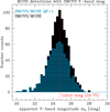 |
Fig. 1. Histogram of the V-band magnitudes assigned by SMUVS to our MUSE detected sources. The peak of the distribution shows the magnitude after which the number counts of MUSE drop significantly. |
Out of 2997 SMUVS objects present in the area covered by MUSE, we managed to successfully identify 1038 objects spectroscopically. All redshifts have been measured and agreed upon by two independent observers, following the work philosophy adopted in, for example, the zCOSMOS spectroscopic survey (Lilly et al. 2007).
Also similarly to zCOSMOS, we classify the quality of our spectra by applying the following quality flags (QFs):
-
−99: non-detection;
-
0: galactic stars, independently of the spectral quality;
-
1: redshift measurement is only tentative;
-
2: relatively secure redshift measurement, with the spectrum showing faint line(s) and/or a continuum, for which the redshift is likely to be correct;
-
3: very secure redshift measurement, typically based on more than one emission line and/or a clear continuum with absorption lines;
-
4: text-book spectrum with emission and absorption lines, and a very clear continuum;
-
9: redshift based on a single but clearly detected emission line, for which we are unsure about its identification. In these cases, a few alternative spectroscopic redshift values are possible for the source.
The MUSE detection rate for the whole SMUVS sample is ∼35% (= 1038/2997), considering all detections regardless of their QF. Among these objects, a total of 691 have a spectroscopic redshift measurement with QF ≥ 2, i.e., ∼23% of all the SMUVS sample in the COSMOS/MUSE GTO field, with the following distribution: 49 galaxies have QF = 2; 486 have QF = 3; 25 have QF = 4; and 131 are classified with QF = 9, as shown in the lower panel of Fig. 2. Furthermore, we also detected 41 stars (QF = 0) and 306 galaxies for which the MUSE data quality is not good enough to constrain the redshift of the object with a high enough confidence level (QF = 1). The remaining 1959 SMUVS objects are non-detections in MUSE.
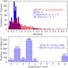 |
Fig. 2. Upper panel: redshift distribution of our sample of SMUVS/MUSE sources with spectral QF ≥ 2 in blue. These objects constitute ∼ 66.5% of the 1038 SMUVS objects identified with MUSE, and ∼23% of all the SMUVS objects in the COSMOS/MUSE GTO field. The distribution of all the SMUVS redshifts in our MUSE fields is drawn in red and renormalized to the number of MUSE sources detected with QF ≥ 2. Lower panel: distribution of spectral QF for the 1038 MUSE detected sources. The dashed line indicates the boundary between a secure and an uncertain redshift measurement. Quality flag 0 was assigned to all galactic stars, independently of their actual spectral quality. |
The upper panel of Fig. 2 shows the redshift distribution of our SMUVS/MUSE sources in blue and the zphot distribution of all the SMUVS sources in the COSMOS/GTO field in red. The SMUVS histogram has been renormalized to match the SMUVS/MUSE sample numbers. As is evident, most of the SMUVS/MUSE detections are located at low redshifts with two overdensities at z ∼ 0.7 and z ∼ 0.9, which belong to previously identified large-scale structures in the COSMOS field (Le Fèvre et al. 2005; Kovač et al. 2010). Since the MUSE data is shallow, it is natural that we only see the brighter sources at higher redshifts. We can also see that the MUSE detections clearly identify the overdensities, and favor redshifts where strong emission lines are present in the MUSE wavelength range (i.e., [OII] between ∼0.2 and ∼1.4 and Lyα above z = 2.9). This is in contrast with the photometric redshift distribution, whose intrinsic dispersion smooths out the peaks, making it less suitable to identify preferential redshifts.
Among the SMUVS sources with MUSE QF ≥ 2 there are 39 with spectroscopic redshift zspec ≥ 2. These include three sources in the redshift range 2 ≤ z < 3 and 36 with redshifts z ≥ 3. The 2 ≤ z < 3 sources consist of two bright galaxies with absorption lines and one AGN with broad CIV and [CIII] emission; the z ≥ 3 sources are prominent Lyα emitters. If we compare the blue and red histograms in Fig. 2, we can see that the MUSE incidence is comparable to SMUVS until z > 4. For the higher redshift, it is the SMUVS relative incidence that is more pronounced.
At 1.5 ≲ z ≲ 3 the number of identified SMUVS/MUSE objects is drastically lower than at higher redshifts. This is known as the “redshift desert”, where no strong nebular emission line falls into the wavelength range covered by MUSE, and thus makes detection particularly difficult. This is clearly illustrated if we look at the number of sources identified in SMUVS in the same redshift range (see red histogram in Fig. 2).
Table 1 shows the results of our redshift measurements for our high-redshift (zspec ≥ 2) sample. We list the SMUVS ID and position of the objects, as well as the spectroscopic redshifts measured and the quality flag assigned to their spectra. There are three sources with QF = 2, additional 20 sources with QF = 3, and 16 sources with QF = 9. For some of the latter, the ambiguity in the single emission line identification could be solved via the available photometric redshifts of these sources (Deshmukh et al. 2018), as will be discussed in Sect. 3.3. We also note that one of our objects (no. 73761) has a previous spectroscopic redshift identification obtained with MOSFIRE on the Keck Telescope (Kriek et al. 2015), and that our own redshift is in good agreement with this previous value (zMOSFIRE = 3.0768). All the remaining spectroscopic redshifts listed here are new (i.e. they are not present in the existing spectroscopic catalogs for the COSMOS field).
SMUVS high-redshift (z ≥ 2) sources identified in the COSMOS/MUSE GTO field.
3.2. MUSE spectra
We focused our attention on the spectra of the 39 galaxies that have zspec ≥ 2.0. We separated the Lyα emitters from absorption line galaxies and AGNs, ending up with 36 sources at z ≳ 3 and 3 sources at redshift 2 ≤ z ≤ 3, as described above.
3.2.1. Lyman-α emitters
We extracted the spectra of our Lyα emitters by identifying the extended area of the line emission. This area is defined by the pixels that have a signal-to-noise ratio higher than three. In order to account for the instrument PSF, we also required a minimum area of 50 pixels. We then added the flux from the single pixels in the area of emission. Finally, we fitted one or two Gaussians to the obtained spectrum and measured the observed flux of the line.
Table 2 contains our line flux measurements, along with the luminosity of the Lyα line derived using the flux and the redshift measured for our objects. We measured the line flux by fitting our data with a number of Gaussians depending on the line profile shown in the spectrum. We then integrated the Gaussians in the wavelength interval containing the line to get the value of the flux reported in Table 2. The mean signal-to-noise ratio of our lines is ∼9.3, with values spanning from 2.5 to 30. The luminosities we measured are on the order of 1042 − 1043 erg s−1, in line with the values published for MUSE-Wide data in other fields (Herenz et al. 2017, 2019).
Measured Lyα fluxes and luminosities for our SMUVS/MUSE sources.
Finally, we note that three different line profiles can be identified in our sample: a single-line profile, where the emission appears mostly symmetric; a blue bump profile, where in addition to the main more intense line a secondary peak in the blue is visible; and a red tail profile, where the emission is either asymmetric with an extended tail in the red part of the spectrum or presents a secondary peak in the red. Figure 3 shows the zoomed-in region of the spectra in the Lyα wavelength range. The plots in the figure also show that we cannot detect a continuum level in our data, thus we are not able to recognize P Cygni profiles, even if they are commonly observed for low-redshift objects. For the three profiles that we recognize, we report the following statistics. Out of 36 objects, 17 show a single-line profile (∼47%), 7 show a blue bump (∼19%), 11 show a red tail (∼31%), and 1 shows both a blue bump and a red tail (∼3%).
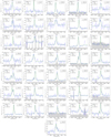 |
Fig. 3. Zoomed-in image of the spectra of our MUSE/SMUVS Lyα emitters. The wavelength range is chosen so that the Lyα line is visible and centered in the plot. The fit is performed by extracting the spectrum from the MUSE data cube in the region where the Lyα emission is ∼3σ above the background or covers at least 50 pixels. The number of Gaussians used in the fit is determined after visual inspection of the shape of the spectrum and serves purely to measure the flux. All three line profiles are represented here. |
The different profiles are caused by the condition and state of the medium in and around the galaxy. For example, a narrow single line can be caused by a reduced amount of scattering for the Lyα photons due to a low hydrogen column density. The blue bump can be caused either by re-emission by the medium of blueshifted Lyα photons or by a strong absorption at the resonant wavelength, leaving only the red tail and a fraction of the original emission. Finally, the red tail can give us information on the offset velocity of the medium, its optical depth, and the hydrogen column density. Radiative transfer models like the ones by Verhamme et al. (2008) or the more recent ones by Gronke (2017) can help disentangle the state of the gas and dust around the emitting galaxy. Applying such models is, however, outside of the scope of this paper, mainly due to the high noise in our spectra, and is left for follow-up studies.
3.2.2. SMUVS/MUSE sources at 2 ≤ z ≤ 3
In addition to the 36 Lyα emitters, we identified 3 other high-redshift objects in the range 2 ≤ z ≤ 3. Object 75267 is an absorption line galaxy at redshift z = 2.4796, classified as a QF = 2 spectrum. We report seeing the CIV doublet in absorption. Object 78359 is classified as a QF = 3 AGN at redshift z = 2.1458 with broad-line emission of both [CIII] and CIV indicating the AGN activity. And finally, object 78448 is a galaxy at redshift z = 2.1723 with QF = 2 emitting CIII and with possible FeII absorptions.
3.3. Physical properties of the SMUVS MUSE galaxies inferred from broadband photometry
We investigate the distribution of properties derived from SED fitting for our sample. Since the physical properties of each object are derived from SMUVS photometry by fitting its SED, we first need to check whether the redshift measured with MUSE matches the photometric redshifts originally derived by Deshmukh et al. (2018).
Out of the 691 SMUVS/MUSE sources for which we measured spectroscopic redshifts with high confidence, we find that 624 sources have a redshift compatible with the photometric value, while 62 are outliers. To define outliers we follow the same definition used by Deshmukh et al. (2018), i.e.,
where zspec is our spectroscopic redshift, while zphot is the photometric redshift of the SMUVS catalog.
Here we find a percentage of outliers of ∼10%, which is somewhat larger than was found in Deshmukh et al. (2018) when comparing all their photometric redshifts with the available COSMOS spectroscopic redshifts, over the whole SMUVS/COSMOS area (the outlier fraction there was 5.5%). This difference is perhaps not surprising, given that there is no source pre-selection in MUSE, while spectra taken with all other spectrographs are preferentially available for bright sources (for which the photometry has a higher signal-to-noise ratio, and thus the photometric analysis is more likely to yield good redshifts). In any case, it is reassuring that the percentage of redshift outliers that we obtain here is still reasonably low.
Before considering the SED fitting properties of our galaxies, we investigated the reason of the redshift discrepancies among the outliers. We focused on the z ≥ 2 sources, which are the main interest here. Among the 39 high-redshift sources, we found 24 for which the photometric and spectroscopic redshifts are in good agreement. We analyzed the remaining 15 cases on an individual basis, in order to understand whether there is any problem in the spectroscopic and/or photometric analysis, or whether the SMUVS/MUSE sources matching is correct. For eight of the outliers we found that the photometry is contaminated by a brighter neighbor; for the other seven we found no apparent photometric contamination. The redshift discrepancy is produced by either the galaxy being fainter than the limiting magnitude of the survey (four cases) or the SMUVS detection actually being two unresolved, separate sources (three cases). In the first situation the photometry of the source is likely unreliable in some bands and in the second case both sources influence the values measured in the photometry, but only one of them emits Lyα and is detected in MUSE. In both cases the photometric fit results in lower zphot in comparison to the zspec.
As the next step, we redid the SED fitting of our high-redshift galaxies with uncontaminated photometry, fixing their redshifts to the MUSE-based spectroscopic value. We used the code LePhare1 (Arnouts et al. 1999; Ilbert et al. 2006), with the same template family and parameter values as in Deshmukh et al. (2018), and considered the same SMUVS 28-band input catalog. We then reran LePhare with fixed redshifts also on the sources that did not show a severe contamination, and found that six of them could be recovered. We thus obtained a final sample of 30 sources (instead of the previous 24) with physical properties derived from photometry, 28 of which are MUSE Lyα emitters.
We see that the SMUVS/MUSE sources have extinction values between 0.0 ≤ E(B − V)≤0.3, with ∼70% having E(B − V)≤0.1, as we would expect from systems that show prominent Lyα lines. Nonetheless, there are still sources that have higher extinctions (0.2 ≤ E(B − V)≤0.3), hinting at an even higher unattenuated Lyα luminosity in those cases. The stellar mass range covered by our sources is from ∼1.5 × 10⁸ M⊙ to ∼7 × 10¹¹ M⊙, with a mean value of ∼109 M⊙. Finally, we see that our objects have ages ranging from 10 Myr to 2 Gyr.
In the next subsection we compare the distribution of the derived SED properties for the Lyα emitters and other SMUVS sources with z ≥ 2.9 (see also Fig. 4).
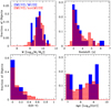 |
Fig. 4. Histogram of the three main properties (age, extinction, and stellar mass) derived from the SMUVS photometry and the redshifts measured by MUSE. We compare our sample of 28 Lyα emitters to the SMUVS sample of complementary high-z objects (218 galaxies). |
3.4. Comparison of SED properties for SMUVS galaxies with and without MUSE identification
We compare the derived SED properties of the SMUVS z > 2.9 sources identified with MUSE (i.e., those with a spectroscopic redshift measurement with QF ≥ 2) with those of the SMUVS z ≳ 2.9 galaxies that are not MUSE-detected, in the same field. Our aim is to investigate whether there are significant differences in these properties, in particular to understand whether the most prominent Lyα emitters at z > 3 are characterized by special values in their physical properties (stellar mass, star formation histories, dust extinction, etc.).
Prior to comparing the SED properties of our objects, we tested whether SMUVS/MUSE and SMUVS/notMUSE galaxies come from the same parent absolute-magnitude distribution. The sample of galaxies we consider is 218 SMUVS galaxies with redshift 2.9 ≲ zphot ≲ 7 and the 28 MUSE Lyα emitters for which our spectroscopic redshifts and the SMUVS photometric redshift estimates are in good agreement (as defined in Sect. 3.3). The comparison is performed on all 28 photometric bands available to SMUVS separately. We performed a Kolmogorov–Smirnov (KS) test on the statistics of the absolute magnitudes derived with LePhare for our two samples. The results of these tests are that the D parameter assumes values ≲0.25 over all the bands tested, and the p-value is always ≥0.08. This indicates that our SMUVS high-redshift MUSE-detected and non-detected sources show no statistically significant difference.
To test whether the sample size can influence the outcome of the test, we reduced the SMUVS sample randomly 10 000 times to subsamples containing an average of 40 objects. The KS test is then performed on these smaller samples and the results are compared to the test on the whole SMUVS sample by means of their statistics. We conclude that sample size does not matter statistically in our case.
Figure 4 shows the distribution of the physical properties of our two samples derived from the SED fit. As can be expected, the redshift distribution of both samples is biased towards lower redshifts in the range 2.9 ≤ z < 6.6 covered by MUSE. The distribution of the stellar mass for our SMUVS/MUSE sample is between 8 < log10(M*) < 11, with a peak at ∼109.5 M*. This sample is also mostly composed of galaxies with little dust content. Nevertheless, some of our objects have E(B − V) > 0.25 and are still visible as Lyα emitters. Unless the emission is seen through a gap in the dust distribution, this would make them extremely bright in Lyα to overcome such higher values of dust extinction and still be visible. Finally, the age distribution exhibits a bimodality, either classifying our galaxies as very young (≲100 Myr) or ∼1 Gyr old. We comment further on this feature in the next subsection. Figure 4 confirms our previous analysis on the input photometric bands used in SMUVS: The distribution of the properties of the SMUVS/MUSE and SMUVS/notMUSE sample are not statistically different.
After we performed a KS test on the physical properties, we concluded that, compared to the SMUVS/notMUSE sample, the spectroscopically detected galaxies generally have lower dust extinction, about the same mass and age distributions, and fewer objects are detected in higher redshift regimes (4 ≤ z ≤ 6.6), but we see no significant statistical difference in any of the properties. The individual results of our KS tests can be seen in Table 3.
Results of all the KS tests performed in this work.
To further test the distribution of the physical properties in both samples, we constructed Fig. 5. We restricted ourselves to analyzing galaxies in the redshift range ∼(3, 4), to limit the effect of galaxy evolution with redshift and because most of the SMUVS/MUSE objects lie in that range. We then also stellar mass matched the SMUVS/notMUSE galaxies to SMUVS/MUSE. The redshift cut applies to all the panels, while the mass matching is shown only for the extinction and the ages. We can see how the age distribution appears very similar in the two samples and how the distribution of redshift and masses do not deviate much from what we saw in Fig. 4, before the redshift cut was applied. The interesting panel is the one showing the extinction. We can see now how applying a cut in redshift and stellar mass matching the SMUVS/notMUSE sample reveals a slight difference in the distribution. SMUVS/MUSE shows preferentially lower extinctions compared to SMUVS/notMUSE, which deviates from E(B − V) > 0.2 onward and drives the difference. Again, the results of a formal KS test can be seen in Table 3.
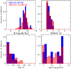 |
Fig. 5. Redshift cut and new stellar mass distribution due to the cut as they were before the mass matching in the upper panels. The mass matched histograms of the extinction E(B − V) and the age derived from the SMUVS photometry for 23 SMUVS/MUSE and 146 SMUVS/notMUSE sources in the redshift range 3 ≤ z ≤ 4 are shown in the lower panels. |
3.5. Further study of the age bimodality
We study the implications of an age bimodality in our MUSE-detected SMUVS sample by comparing the stellar mass–age and E(B − V)–age relations of SMUVS/MUSE to the relations found in SMUVS/notMUSE (see Fig. 6). We can see, as is expected from the current view on galaxy evolution, that the younger objects tend to be less massive than the older objects and that they are in general more obscured than older objects. We associate these characteristics with the fact that the younger galaxies in our sample are currently experiencing their first star formation event. The older objects in contrast have already formed the bulk of their stars, and thus show older populations and have less dust in their surroundings.
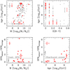 |
Fig. 6. Upper panels: mass–age relation on the left and E(B − V)–age relation on the right for both our SMUVS detected samples. Here, SMUVS/MUSE is represented in red, while SMUVS/notMUSE is plotted in gray. We see that the older objects are generally more massive and that the younger objects experience generally more extinction than older objects. Lower panels: test of the lower limit of the instantaneous SFR derived from our Lyα flux measurements against an average star formation rate obtained by dividing the stellar mass by the age of the galaxy obtained from the SED fit. We see on the left that the higher SFR is associated with intermediate-mass objects, and on the right that older objects have a higher SFR than what would be expected if they had continuously formed stars in one single episode. The gray line in the plots indicates where the ratio between SFRs is unity. The error bars shown in the plots are representative of the average errors on the galactic properties. |
We notice however that all SMUVS/MUSE objects are detected in Lyα emission and so we expect them to be actively star-forming. We argue that the star formation that we see in the older objects is not part of the first event, but a separated second episode of star formation. To test this, we generated the lower plots in Fig. 6. We compare the SFR obtained if we assume a continuous star formation throughout the lifetime of our objects and the lower limit of the SFR given by the Lyα emission we detect. The first value is obtained by dividing the stellar mass given by the SED fit with the age of the galaxy and represents the average of the SFR. The second value is obtained by applying the conversion  , which gives us a lower limit for the luminosity in the Hα line and for which we chose to use the Lyα−Hα conversion factor by Hu et al. (1998). We then use the Kennicutt (1998) equation to obtain the SFR from the Hα luminosity to obtain the lower limit of the instantaneous SFR.
By comparing these two values we can qualitatively say whether a galaxy is consistent with a monotonically declining star formation history (SFRinstant/SFRaverage ≤ 1) or if a second star formation episode is needed to explain the SFR (SFRinstant/SFRaverage > 1). We see that galaxies that are experiencing a second event are intermediate-mass objects (9 ≲ log10(M*)≤10) and are exclusively old. We argue that the main component of the stellar population has formed in early times with the first star formation event and is what the SMUVS photometry detects, while the new stars being formed are detected by MUSE. We conclude that these objects are probably experiencing a rejuvenation event, and that their star formation restarted after the stellar bulk was formed, about 1 Gyr before the time we observe them.
3.6. Additional MUSE high-redshift sources not present in SMUVS
Additionally to the Lyα emitters in the SMUVS/MUSE sample, we also performed a blind search in the MUSE cubes and found 66 other sources presenting a secure or possible Lyα emission (QF = 2, 3, and 9). These new sources (hereafter MUSE/NS) have been identified by visually inspecting the MUSE data cubes, and do not have a previous spectroscopic confirmation. We also verified that, in the specific framework of our analysis, performing an automated search in our cubes (i.e., by using the software LSDCat, Herenz & Wisotzki 2017) rather than a visual one would not add new sources to our secure detections (QF > 1). Since the MUSE/NS sample is not present in the SMUVS catalog, we have information on the redshift and measurements of the Lyα flux and luminosity, but no estimate of the physical properties of these objects from SED fitting. The MUSE/NS sources and all their related quantities are listed in Table B.1.
To test whether these objects belong to a different population from the galaxies selected in SMUVS, we verified that none of these new sources was situated in masked areas of the survey. In fact, 61 of them were never selected for the catalog to begin with and 5 have a SMUVS neighbor within 1″, but are clearly different objects. Since the SMUVS galaxies were detected based on a prior selection in the UltraVISTA HKs stacks, we conclude that these MUSE/NS sources are faint in the HKs stacks and/or in the images from the Spitzer 3.6 μm and 4.5 μm bands.
Given that the UltraVISTA images are deep, we can safely assume that the reason these objects are undetected is that they are below the mass limit of the survey. Even without having performed an SED fit, we can state that the MUSE/NS sample will likely have a very different mass distribution compared to the SMUVS/MUSE sample. This is likely the source of the discrepancies we find between the two populations. We put an upper limit on their stellar mass by citing the 50% completeness limit reported in Table 1 of Deshmukh et al. (2018). For galaxies in 3.0 ≤ z ≤ 4.0 the upper limit mass is log10(M*/M⊙) = 9.0, for the range 4.0 < z ≤ 5.0 it is 9.2, and finally for galaxies with 5.0 < z ≤ 6.0 it is 9.4.
We measured the Lyα emission and luminosity for the MUSE/NS sample in the same way as we did for the SMUVS/MUSE sources. The first difference we noticed is that the number of blue bump profiles is strongly reduced compared to the SMUVS/MUSE sample (2/66 against 7/36, or ∼3% against ∼19%). Furthermore, the single-line profile appears in 44 spectra, constituting ∼67% of the sample, which makes it more prominent than in the SMUVS/MUSE sample, where it was observed ∼47% of the time. Finally, the red tail profile appears in 20 of our galaxies and is about as frequent as in the SMUVS/MUSE sample (MUSE/NS ∼30%, SMUVS/MUSE ∼31%). If we compare SMUVS/MUSE to MUSE/NS, both in line flux and luminosity using a KS test, we see that their distributions are different and that MUSE/NS are the fainter objects. This confirms the fact that blue bump profiles are harder to detect, and thus the single-line profiles increase in number for the fainter sources. Further evidence for this interpretation is that the blue bump objects are found in the brighter objects located at 3 ≤ z < 4 of the SMUVS/MUSE (green circles in Fig. 7). The results of these KS tests can again be found in Table 3.
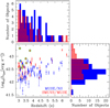 |
Fig. 7. Upper panel: comparison in redshift distribution between the SMUVS sources (red) and the sources identified in the Blind search (blue). Left panel: Lyα luminosity plotted as a function of redshift for our sources. The green circles identify the blue bump objects. Right panel: histogram of the measured luminosities for both our samples. The blind search objects show slightly fainter luminosities compared to the SMUVS sources. |
The right panel of Fig. 7 illustrates this trend by showing the distribution of LLyα for the two samples. We also plotted their distribution in redshift and how their luminosity evolves with it, in the upper and left panel of Fig. 7, respectively. We see in the central panel of Fig. 7 that for both samples the measured Lyα luminosity plotted against redshift increases with it, as can be expected given the detection limit on the line flux. More interestingly, the MUSE/NS sources seem to lie close enough in redshift space to the SMUVS/MUSE sources, suggesting they could belong to the same physical structure. To test if this is the case, we defined a Δz dependent on redshift, such that two objects with said distance in redshift lie 2 Mpc apart. We then expanded our check also to the position on the sky and defined a sphere of 2 Mpc radius as our criterion to check for associations.
We find that we can identify nine associations in the area covered by MUSE. If we restrict ourselves to only considering QF = 3, 4 objects, then the number of associations we find drops to three (see Table 4). We compared the number of associations we find with MUSE in our small area to the number of associations we could find in the part of the COSMOS field covered by SMUVS using spectroscopic confirmed objects currently known in the literature. We chose spectroscopic sources with QF = 3, 4 only and applied the same criteria used on the MUSE data to identify associations. We find 16 associations over the entirety of the SMUVS/COSMOS field. If we assume that the MUSE rate in our small area is indicative of what we could find if MUSE covered SMUVS/COSMOS entirely, then we would expect to find ∼360 associations in this larger area. Unless cosmic variance is playing a big role in the area MUSE covered in our data, we estimate that MUSE has a ∼20× higher chance of detecting objects that could be physically linked, confirming the usefulness of MUSE for unbiased source detection.
Position and redshift of the three secure associations identified via our method.
4. Summary and conclusions
We made use of publicly available MUSE data in the COSMOS field to analyze a sample of 2997 photometrically selected galaxies from the SMUVS survey over an area of 20.79 arcmin2. We managed to detect and measure the redshift of 691 objects, of which 39 are located at z ≥ 2. For these sources, we report two absorption line galaxies and one AGN in addition to 36 Lyman-α emitters. Of these 39 sources, all but 1 are new redshift measurements not previously present in the literature. Furthermore, we identify 66 additional Lyα emitters by performing a blind search in the MUSE cubes. The values we measured for the Lyα flux and luminosity of our sources are in line with other works using MUSE pointings with similar depth and conditions (Herenz et al. 2017, 2019). We also detect three different line profiles in our combined Lyα sample, hinting at different medium conditions in and around our objects. A quantitative analysis of these features was, however, beyond the scope of this paper, whose goal was instead to investigate the differences in physical properties between the sources identified in the SMUVS catalog also detected in MUSE and those that could not be detected in MUSE.
The main result of our paper is to compare the physical properties of the SMUVS/MUSE and SMUVS/notMUSE sources. While there are some differences in the distribution of E(B − V), stellar mass, and age in the two samples, we find that their overall distribution does not vary substantially. We know that the SMUVS catalog is more sensitive to the brighter, more massive galaxies. MUSE instead has the only bias of being able to select objects that are at least bright enough in line emission to be detected. For z > 2.9 galaxies, this means they are bright Lyα emitters, intense star-forming objects with little dust attenuation/HI absorption. Not finding a significant difference in physical properties between our two samples, even after applying a redshift cut and mass matching them, could imply that the SMUVS selected Lyα emitters we observe in MUSE are similar to the general population in SMUVS. Although SMUVS is not the largest nor deepest survey in COSMOS, it is the Spitzer survey with the largest area for its depth (only shallower than CANDELS, which covers an area 12 times smaller in COSMOS). We can thus probe a sample of galaxies that is more complete in parameter space than ever before.
After mass matching our samples, we see that SMUVS/MUSE is less obscured than SMUVS/notMUSE. We also note how the age distribution of our Lyα emitters shows a bimodality. Both these results have been found in other studies where Lyα information has been combined with photometric SED fitting (Lai et al. 2008; Finkelstein et al. 2009; Pentericci et al. 2009). Furthermore, we deepened our study of the bimodality in the age of our sample by studying the SFR of our objects qualitatively. We find that the younger objects are most likely experiencing their first burst of star formation. The older objects in our sample show instead a lower limit to their instantaneous SFR, derived from their Lyα luminosity, that suggests they are undergoing a second burst of star formation, while the light of the galaxy is dominated by an older population of stars. This rejuvenation effect has also recently been observed in low-redshift objects by Angthopo et al. (2019) and Cooke et al. (2019).
We also compared the SMUVS/MUSE and MUSE/NS samples. Using MUSE data allowed us an unbiased detection of all the sources that are bright in Lyα. We were able to perform a blind search in the MUSE cubes and enlarge our sample of Lyα emitters by a factor of ∼3. MUSE thus confirms its potential for systematic searches of a given area in the sky. This sensitivity to emission lines also allowed us to detect three secure and previously undiscovered physical galaxy associations.
What is puzzling, however, is that MUSE detects MUSE/NS objects at luminosities around 1042 erg s−1 and below, but does not detect such lower luminosities for the SMUVS/MUSE sample (see right histogram in Fig. 7). We determined that the MUSE/NS sample lies most likely below the mass completeness limit of the SMUVS survey. We note, however, that the Lyα luminosities of the MUSE/NS sample have a significant overlap with the SMUVS/MUSE luminosities. Since the Lyα line intensity is linked to the ionizing radiation emitted and not the mass of the object, this overlap is not surprising. It does, however, point out that we cannot attribute the lack of lower luminosity SMUVS/MUSE objects to a simple scaling effect due to the mass-selection in SMUVS. At present we do not have a definitive solution for this issue.
The area of improvement in this study is the depth of the pointings. Longer exposure times could yield a higher detection rate for the SMUVS selected sources (to date about 2/3 could not be detected) and deep enough spectra to measure a continuum. This would allow us to more accurately investigate the line shapes (we could distinguish P Cygni profiles from single lines) and also measure equivalent widths for the brighter objects.
Acknowledgments
The authors would like to thank the anonymous referee for the helpful and constructing feedback. GR, GBC, KIC and SD acknowledge funding from the European Research Council through the award of the Consolidator Grant ID 681627-BUILDUP. Based on observations collected at the European Southern Observatory under ESO Programme IDs 095.A-0240(A), 096.A-0090(A), 097.A-0160(A), 098.A-0017(A). Also based in part on observations carried out with the Spitzer Space Telescope, which is operated by the Jet Propulsion Laboratory, California Institute of Technology under a contract with NASA. This research made use of Astropy, (http://www.astropy.org) a community-developed core Python package for Astronomy (Astropy Collaboration 2013, 2018).
References
- Acquaviva, V., Vargas, C., Gawiser, E., & Guaita, L. 2012, ApJ, 751, L26 [NASA ADS] [CrossRef] [Google Scholar]
- Angthopo, J., Ferreras, I., & Silk, J. 2019, MNRAS, 488, L99 [NASA ADS] [CrossRef] [Google Scholar]
- Arnouts, S., Cristiani, S., Moscardini, L., et al. 1999, MNRAS, 310, 540 [NASA ADS] [CrossRef] [Google Scholar]
- Ashby, M. L. N., Caputi, K. I., Cowley, W., et al. 2018, ApJS, 237, 39 [NASA ADS] [CrossRef] [Google Scholar]
- Astropy Collaboration (Robitaille, T. P., et al.) 2013, A&A, 558, A33 [NASA ADS] [CrossRef] [EDP Sciences] [Google Scholar]
- Astropy Collaboration (Price-Whelan, A. M., et al.) 2018, AJ, 156, 123 [Google Scholar]
- Bacon, R., Accardo, M., Adjali, L., et al. 2010, in Ground-based and Airborne Instrumentation for Astronomy III, Proc. SPIE, 7735, 773508 [CrossRef] [Google Scholar]
- Bacon, R., Piqueras, L., Conseil, S., Richard, J., & Shepherd, M. 2016, Astrophysics Source Code Library [record ascl:1611.003] [Google Scholar]
- Bertin, E., & Arnouts, S. 1996, A&AS, 117, 393 [NASA ADS] [CrossRef] [EDP Sciences] [Google Scholar]
- Bridge, J. S., Hayes, M., Melinder, J., et al. 2018, ApJ, 852, 9 [NASA ADS] [CrossRef] [Google Scholar]
- Caputi, K. I., Cirasuolo, M., Dunlop, J. S., et al. 2011, MNRAS, 413, 162 [NASA ADS] [CrossRef] [Google Scholar]
- Caputi, K. I., Deshmukh, S., Ashby, M. L. N., et al. 2017, ApJ, 849, 45 [NASA ADS] [CrossRef] [Google Scholar]
- Cooke, K. C., Kartaltepe, J. S., Tyler, K. D., et al. 2019, ApJ, 881, 150 [NASA ADS] [CrossRef] [Google Scholar]
- Cowley, W. I., Caputi, K. I., Deshmukh, S., et al. 2018, ApJ, 853, 69 [NASA ADS] [CrossRef] [Google Scholar]
- Cowley, W. I., Caputi, K. I., Deshmukh, S., et al. 2019, ApJ, 874, 114 [NASA ADS] [CrossRef] [Google Scholar]
- Curtis-Lake, E., McLure, R. J., Dunlop, J. S., et al. 2013, MNRAS, 429, 302 [NASA ADS] [CrossRef] [Google Scholar]
- De Barros, S., Pentericci, L., Vanzella, E., et al. 2017, A&A, 608, A123 [NASA ADS] [CrossRef] [EDP Sciences] [Google Scholar]
- Deshmukh, S., Caputi, K. I., Ashby, M. L. N., et al. 2018, ApJ, 864, 166 [NASA ADS] [CrossRef] [Google Scholar]
- Diener, C., Wisotzki, L., Schmidt, K. B., et al. 2017, MNRAS, 471, 3186 [NASA ADS] [CrossRef] [Google Scholar]
- Dijkstra, M. 2017, ArXiv e-prints [arXiv:1704.03416] [Google Scholar]
- Erb, D. K., Steidel, C. C., & Chen, Y. 2018, ApJ, 862, L10 [NASA ADS] [CrossRef] [Google Scholar]
- Fazio, G. G., Hora, J. L., Allen, L. E., et al. 2004, ApJS, 154, 10 [NASA ADS] [CrossRef] [Google Scholar]
- Finkelstein, S. L., Rhoads, J. E., Malhotra, S., & Grogin, N. 2009, ApJ, 691, 465 [NASA ADS] [CrossRef] [Google Scholar]
- Grogin, N. A., Kocevski, D. D., Faber, S. M., et al. 2011, ApJS, 197, 35 [NASA ADS] [CrossRef] [Google Scholar]
- Gronke, M. 2017, A&A, 608, A139 [Google Scholar]
- Guaita, L., Acquaviva, V., Padilla, N., et al. 2011, ApJ, 733, 114 [NASA ADS] [CrossRef] [Google Scholar]
- Gurung-Lopez, S., Orsi, A. A., & Bonoli, S. 2019, MNRAS, 490, 733 [NASA ADS] [CrossRef] [Google Scholar]
- Hao, C.-N., Huang, J.-S., Xia, X., et al. 2018, ApJ, 864, 145 [NASA ADS] [CrossRef] [Google Scholar]
- Herenz, E. C., & Wisotzki, L. 2017, A&A, 602, A111 [NASA ADS] [CrossRef] [EDP Sciences] [Google Scholar]
- Herenz, E. C., Urrutia, T., Wisotzki, L., et al. 2017, A&A, 606, A12 [NASA ADS] [CrossRef] [EDP Sciences] [Google Scholar]
- Herenz, E. C., Wisotzki, L., Saust, R., et al. 2019, A&A, 621, A107 [NASA ADS] [CrossRef] [EDP Sciences] [Google Scholar]
- Hernán-Caballero, A., Pérez-González, P. G., Diego, J. M., et al. 2017, ApJ, 849, 82 [NASA ADS] [CrossRef] [Google Scholar]
- Hu, E. M., Cowie, L. L., & McMahon, R. G. 1998, ApJ, 502, L99 [NASA ADS] [CrossRef] [Google Scholar]
- Ilbert, O., Arnouts, S., McCracken, H. J., et al. 2006, A&A, 457, 841 [NASA ADS] [CrossRef] [EDP Sciences] [Google Scholar]
- Kakiichi, K., & Gronke, M. 2019, ApJ, submitted [arXiv:1905.02480] [Google Scholar]
- Karman, W., Caputi, K. I., Trager, S. C., Almaini, O., & Cirasuolo, M. 2014, A&A, 565, A5 [NASA ADS] [CrossRef] [EDP Sciences] [Google Scholar]
- Karman, W., Caputi, K. I., Caminha, G. B., et al. 2017, A&A, 599, A28 [NASA ADS] [CrossRef] [EDP Sciences] [Google Scholar]
- Kennicutt, Jr., R. C. 1998, ARA&A, 36, 189 [Google Scholar]
- Kimm, T., Blaizot, J., Garel, T., et al. 2019, MNRAS, 486, 2215 [NASA ADS] [CrossRef] [Google Scholar]
- Koekemoer, A. M., Faber, S. M., Ferguson, H. C., et al. 2011, ApJS, 197, 36 [NASA ADS] [CrossRef] [Google Scholar]
- Kovač, K., Lilly, S. J., Cucciati, O., et al. 2010, ApJ, 708, 505 [NASA ADS] [CrossRef] [Google Scholar]
- Kriek, M., Shapley, A. E., Reddy, N. A., et al. 2015, ApJS, 218, 15 [NASA ADS] [CrossRef] [Google Scholar]
- Lai, K., Huang, J.-S., Fazio, G., et al. 2008, ApJ, 674, 70 [NASA ADS] [CrossRef] [Google Scholar]
- Le Fèvre, O., Vettolani, G., Garilli, B., et al. 2005, A&A, 439, 845 [NASA ADS] [CrossRef] [EDP Sciences] [Google Scholar]
- Lilly, S. J., Le Fèvre, O., Renzini, A., et al. 2007, ApJS, 172, 70 [NASA ADS] [CrossRef] [Google Scholar]
- Mallery, R. P., Mobasher, B., Capak, P., et al. 2012, ApJ, 760, 128 [NASA ADS] [CrossRef] [Google Scholar]
- Marchi, F., Pentericci, L., Guaita, L., et al. 2019, A&A, 631, A19 [NASA ADS] [CrossRef] [EDP Sciences] [Google Scholar]
- Martin, C. L., Dijkstra, M., Henry, A., et al. 2015, ApJ, 803, 6 [NASA ADS] [CrossRef] [Google Scholar]
- Martinache, C., Rettura, A., Dole, H., et al. 2018, A&A, 620, A198 [NASA ADS] [CrossRef] [EDP Sciences] [Google Scholar]
- Mas-Hesse, J. M., Kunth, D., Tenorio-Tagle, G., et al. 2003, ApJ, 598, 858 [NASA ADS] [CrossRef] [Google Scholar]
- McCracken, H. J., Milvang-Jensen, B., Dunlop, J., et al. 2012, A&A, 544, A156 [NASA ADS] [CrossRef] [EDP Sciences] [Google Scholar]
- McLinden, E. M., Rhoads, J. E., Malhotra, S., et al. 2014, MNRAS, 439, 446 [NASA ADS] [CrossRef] [Google Scholar]
- Nakajima, K., Fletcher, T., Ellis, R. S., Robertson, B. E., & Iwata, I. 2018, MNRAS, 477, 2098 [NASA ADS] [CrossRef] [Google Scholar]
- Ono, Y., Ouchi, M., Shimasaku, K., et al. 2010, MNRAS, 402, 1580 [NASA ADS] [CrossRef] [Google Scholar]
- Orlitová, I., Verhamme, A., Henry, A., et al. 2018, A&A, 616, A60 [NASA ADS] [CrossRef] [EDP Sciences] [Google Scholar]
- Pentericci, L., Grazian, A., Fontana, A., et al. 2009, A&A, 494, 553 [NASA ADS] [CrossRef] [EDP Sciences] [Google Scholar]
- Pentericci, L., Grazian, A., Scarlata, C., et al. 2010, A&A, 514, A64 [NASA ADS] [CrossRef] [EDP Sciences] [Google Scholar]
- Piqueras, L., Conseil, S., Shepherd, M., et al. 2017, ArXiv e-prints [arXiv:1710.03554] [Google Scholar]
- Remolina-Gutiérrez, M. C., & Forero-Romero, J. E. 2019, MNRAS, 482, 4553 [NASA ADS] [CrossRef] [Google Scholar]
- Scoville, N., Aussel, H., Brusa, M., et al. 2007, ApJS, 172, 1 [NASA ADS] [CrossRef] [Google Scholar]
- Shapley, A. E., Steidel, C. C., Pettini, M., & Adelberger, K. L. 2003, ApJ, 588, 65 [NASA ADS] [CrossRef] [Google Scholar]
- Smith, A., Ma, X., Bromm, V., et al. 2019, MNRAS, 484, 39 [NASA ADS] [CrossRef] [Google Scholar]
- Sobral, D., Matthee, J., Darvish, B., et al. 2018, MNRAS, 477, 2817 [NASA ADS] [CrossRef] [Google Scholar]
- Soto, K. T., Lilly, S. J., Bacon, R., Richard, J., & Conseil, S. 2016, MNRAS, 458, 3210 [NASA ADS] [CrossRef] [Google Scholar]
- Taniguchi, Y., Scoville, N., Murayama, T., et al. 2007, ApJS, 172, 9 [NASA ADS] [CrossRef] [Google Scholar]
- Tenorio-Tagle, G., Silich, S. A., Kunth, D., Terlevich, E., & Terlevich, R. 1999, MNRAS, 309, 332 [NASA ADS] [CrossRef] [Google Scholar]
- Urrutia, T., Wisotzki, L., Kerutt, J., et al. 2019, A&A, 624, A141 [NASA ADS] [CrossRef] [EDP Sciences] [Google Scholar]
- Vanzella, E., Nonino, M., Cupani, G., et al. 2018, MNRAS, 476, L15 [NASA ADS] [CrossRef] [Google Scholar]
- Verhamme, A., Schaerer, D., Atek, H., & Tapken, C. 2008, A&A, 491, 89 [NASA ADS] [CrossRef] [EDP Sciences] [Google Scholar]
- Verhamme, A., Garel, T., Ventou, E., et al. 2018, MNRAS, 478, L60 [NASA ADS] [CrossRef] [Google Scholar]
- Weilbacher, P. M., Roth, M. M., Pécontal-Rousset, A., & Bacon, R. 2006, New Astron. Rev., 50, 405 [NASA ADS] [CrossRef] [Google Scholar]
- Weilbacher, P. M., Streicher, O., Urrutia, T., et al. 2012, in Software and Cyberinfrastructure for Astronomy II, Proc. SPIE, 8451, 84510B [CrossRef] [Google Scholar]
- Weilbacher, P. M., Streicher, O., Urrutia, T., et al. 2014, in Astronomical Data Analysis Software and Systems XXIII, eds. N. Manset, & P. Forshay, ASP Conf. Ser., 485, 451 [NASA ADS] [Google Scholar]
- Werner, M. W., Roellig, T. L., Low, F. J., et al. 2004, ApJS, 154, 1 [NASA ADS] [CrossRef] [Google Scholar]
- Yuma, S., Ohta, K., Yabe, K., et al. 2010, ApJ, 720, 1016 [NASA ADS] [CrossRef] [Google Scholar]
- Zhang, H., Ouchi, M., Itoh, R., et al. 2019, ApJ, submitted [arXiv:1905.09841] [Google Scholar]
Appendix A: Complete redshift catalog
Table A.1 shows the first five rows of our complete redshift catalog. We only include all redshift measurements that have QF > 1 in this table.
First five rows of the full redshift catalog for the 20.79 arcmin2 covered by MUSE.
Appendix B: MUSE/NS sources
Table B.1 lists the properties of the 66 Lyα emitters found by performing our blind search.
Blind search detected high-redshift (z ≥ 2.9) Lyα emitting sources in the COSMOS/MUSE GTO field.
All Tables
Position and redshift of the three secure associations identified via our method.
First five rows of the full redshift catalog for the 20.79 arcmin2 covered by MUSE.
Blind search detected high-redshift (z ≥ 2.9) Lyα emitting sources in the COSMOS/MUSE GTO field.
All Figures
|
Fig. 1. Histogram of the V-band magnitudes assigned by SMUVS to our MUSE detected sources. The peak of the distribution shows the magnitude after which the number counts of MUSE drop significantly. |
| In the text | |
|
Fig. 2. Upper panel: redshift distribution of our sample of SMUVS/MUSE sources with spectral QF ≥ 2 in blue. These objects constitute ∼ 66.5% of the 1038 SMUVS objects identified with MUSE, and ∼23% of all the SMUVS objects in the COSMOS/MUSE GTO field. The distribution of all the SMUVS redshifts in our MUSE fields is drawn in red and renormalized to the number of MUSE sources detected with QF ≥ 2. Lower panel: distribution of spectral QF for the 1038 MUSE detected sources. The dashed line indicates the boundary between a secure and an uncertain redshift measurement. Quality flag 0 was assigned to all galactic stars, independently of their actual spectral quality. |
| In the text | |
|
Fig. 3. Zoomed-in image of the spectra of our MUSE/SMUVS Lyα emitters. The wavelength range is chosen so that the Lyα line is visible and centered in the plot. The fit is performed by extracting the spectrum from the MUSE data cube in the region where the Lyα emission is ∼3σ above the background or covers at least 50 pixels. The number of Gaussians used in the fit is determined after visual inspection of the shape of the spectrum and serves purely to measure the flux. All three line profiles are represented here. |
| In the text | |
|
Fig. 4. Histogram of the three main properties (age, extinction, and stellar mass) derived from the SMUVS photometry and the redshifts measured by MUSE. We compare our sample of 28 Lyα emitters to the SMUVS sample of complementary high-z objects (218 galaxies). |
| In the text | |
|
Fig. 5. Redshift cut and new stellar mass distribution due to the cut as they were before the mass matching in the upper panels. The mass matched histograms of the extinction E(B − V) and the age derived from the SMUVS photometry for 23 SMUVS/MUSE and 146 SMUVS/notMUSE sources in the redshift range 3 ≤ z ≤ 4 are shown in the lower panels. |
| In the text | |
|
Fig. 6. Upper panels: mass–age relation on the left and E(B − V)–age relation on the right for both our SMUVS detected samples. Here, SMUVS/MUSE is represented in red, while SMUVS/notMUSE is plotted in gray. We see that the older objects are generally more massive and that the younger objects experience generally more extinction than older objects. Lower panels: test of the lower limit of the instantaneous SFR derived from our Lyα flux measurements against an average star formation rate obtained by dividing the stellar mass by the age of the galaxy obtained from the SED fit. We see on the left that the higher SFR is associated with intermediate-mass objects, and on the right that older objects have a higher SFR than what would be expected if they had continuously formed stars in one single episode. The gray line in the plots indicates where the ratio between SFRs is unity. The error bars shown in the plots are representative of the average errors on the galactic properties. |
| In the text | |
|
Fig. 7. Upper panel: comparison in redshift distribution between the SMUVS sources (red) and the sources identified in the Blind search (blue). Left panel: Lyα luminosity plotted as a function of redshift for our sources. The green circles identify the blue bump objects. Right panel: histogram of the measured luminosities for both our samples. The blind search objects show slightly fainter luminosities compared to the SMUVS sources. |
| In the text | |
Current usage metrics show cumulative count of Article Views (full-text article views including HTML views, PDF and ePub downloads, according to the available data) and Abstracts Views on Vision4Press platform.
Data correspond to usage on the plateform after 2015. The current usage metrics is available 48-96 hours after online publication and is updated daily on week days.
Initial download of the metrics may take a while.