| Issue |
A&A
Volume 627, July 2019
|
|
|---|---|---|
| Article Number | A11 | |
| Number of page(s) | 7 | |
| Section | The Sun | |
| DOI | https://doi.org/10.1051/0004-6361/201935606 | |
| Published online | 25 June 2019 | |
Reconstructing solar magnetic fields from historical observations
IV. Testing the reconstruction method
1
ReSoLVE Centre of Excellence, Space Climate Research Unit, University of Oulu, PO Box 3000, 90014 Oulu, Finland
e-mail: This email address is being protected from spambots. You need JavaScript enabled to view it.
2
National Solar Observatory, Boulder, CO 80303, USA
3
Pulkovo Astronomical Observatory, Russian Academy of Sciences, Pulkovskoye Shosse 65, Saint Petersburg 196140, Russian Federation
4
Department of Mathematical Sciences, Durham University, Durham DH1 3LE, UK
Received:
3
April
2019
Accepted:
28
May
2019
Abstract
Aims. The evolution of the photospheric magnetic field has only been regularly observed since the 1970s. The absence of earlier observations severely limits our ability to understand the long-term evolution of solar magnetic fields, especially the polar fields that are important drivers of space weather. Here, we test the possibility to reconstruct the large-scale solar magnetic fields from Ca II K line observations and sunspot magnetic field observations, and to create synoptic maps of the photospheric magnetic field for times before modern-time magnetographic observations.
Methods. We reconstructed active regions from Ca II K line synoptic maps and assigned them magnetic polarities using sunspot magnetic field observations. We used the reconstructed active regions as input in a surface flux transport simulation to produce synoptic maps of the photospheric magnetic field. We compared the simulated field with the observed field in 1975−1985 in order to test and validate our method.
Results. The reconstruction very accurately reproduces the long-term evolution of the large-scale field, including the poleward flux surges and the strength of polar fields. The reconstruction has slightly less emerging flux because a few weak active regions are missing, but it includes the large active regions that are the most important for the large-scale evolution of the field. Although our reconstruction method is very robust, individual reconstructed active regions may be slightly inaccurate in terms of area, total flux, or polarity, which leads to some uncertainty in the simulation. However, due to the randomness of these inaccuracies and the lack of long-term memory in the simulation, these problems do not significantly affect the long-term evolution of the large-scale field.
Key words: Sun: magnetic fields / Sun: activity / Sun: photosphere / sunspots
© ESO 2019
1. Introduction
Magnetic fields are the source of energy for many forms of solar activity and eruptions, for example flares and coronal mass ejections. They also greatly affect the properties of the solar wind; open field lines of coronal holes being the source of the particle flow. In fact, solar magnetic fields are the driver of all space weather, and their effects can be observed on the surface of the Earth as geomagnetic activity. This makes the understanding of properties and evolution of solar magnetic field a very important and interesting topic.
The first magnetographic full-disk observations of the photospheric magnetic field were made in the 1950s (Babcock 1953). While strong fields in sunspots had been observed earlier (Hale et al. 1919), these were the first observations that covered the whole solar disk, including weak fields. Routine full-disk observations started in the 1970s (Howard 1974; Livingston et al. 1976). This means that we have a good coverage of magnetic field observations for only the last four solar cycles, which severely limits our ability to understand the long-term evolution of the solar magnetic field. Additionally, due to the vantage point effect, even with modern instrumentation it is very difficult to measure the field reliably near the poles, as only one pole is visible at a time, and the line of sight is almost parallel to the surface at the highest latitudes. Therefore, surface flux transport (SFT) models, which can simulate the polar fields if flux emergence at low latitudes is known, can be very helpful.
Sunspot numbers or sunspot areas are often used as a measure of flux emergence when SFT models are used to study the long-term evolution of the magnetic field (Jiang et al. 2010, 2011; Baumann et al. 2004). The shortcoming of this approach is that sunspot numbers or areas alone do not provide any information about the tilt angles of individual active regions, or the distribution of flux in the activity belts in general. These models usually rely on the laws of Hale and Joy to create magnetic bipoles that follow the statistical distribution of these laws, and are then inserted into the simulation. Active regions can also be assimilated directly from magnetographic observations, which offers much more accuracy (Virtanen et al. 2017, 2018; Whitbread et al. 2017, 2018; Yeates et al. 2015). However, magnetographic observations are more limited in time, which means that times before the 1970s cannot be simulated. To extend the simulation further into the past, the active regions must somehow be constructed from other observations.
While full-disk magnetographic observations did not start until the 1950s, routine measurements of the magnetic fields of sunspots began to be taken as early as 1917 at the Mount Wilson observatory (MWO). The sunspot field strength and polarity, along with other observations, were originally written on daily sunspot drawings, which were later digitized and the parameters tabulated (Pevtsov et al. 2019; Tlatov et al. 2015). Two years earlier, in 1915, MWO also started routine daily full-disk observations of the chromospheric Ca II K 393.37 nm spectral line (Hale 1908; Ellerman 1919).
A good spatial correspondence between the bright chromospheric plages and areas of stronger magnetic field around active regions was noted in very early magnetographic observations (Babcock & Babcock 1955; Leighton 1959) and the calcium K line intensity of chromospheric plages serves as a proxy for the unsigned magnetic flux in the photospheric regions below. Combined with the information about the polarity of sunspot magnetic fields, the CaK line intensity allows one to create pseudomagnetograms of active regions starting from 1917 (Pevtsov et al. 2016). These can then be combined with an SFT model to simulate the polar fields for the same time period, resulting in synoptic maps of the modeled magnetic field for times before magnetographic observations.
The purpose of this paper is to study the feasibility and accuracy of the reconstruction described above. We follow the method for reconstructing active regions from calcium K line and sunspot observations first presented in Pevtsov et al. (2016), and use them as input for the SFT model that has previously been tested in Virtanen et al. (2017). To be able to compare our results with observations, we study the time period from 1975 to 1985, as both calcium K line and magnetographic observations are available for these years. The paper is structured as follows. In Sect. 2 we present the three data sets, and Sect. 3 describes the SFT model used in this study. In Sect. 4 we present the active region reconstruction method in detail, and discuss its accuracy. In Sect. 6 we present the simulated photospheric field and compare it with observations. In Sect. 7 we discuss the results and present our conclusions.
2. Data
In this paper, three different data sets are used: synoptic maps of the photospheric magnetic field and of the calcium K line intensity, and sunspot drawings. The calcium K line and sunspot magnetic field data are used to reconstruct the active regions that the SFT simulation uses as input, and the synoptic maps of the photospheric magnetic field are used to validate the simulation.
The photospheric line-of-sight magnetic field has been measured at National Solar Observatory (NSO) at Kitt Peak (KP) since the 1970s. From February 1975 (Carrington rotation (CR) 1625) until March 1992 (CR 1853) the instrument was a 512-channel diode array magnetograph using the Fe I 868.8 nm spectral line (Livingston et al. 1976). From these observations pseudo-radial field synoptic maps are created with a resolution of one degree in longitude and 1/90 in sine of latitude under the assumption that the field is radial in the photosphere. In this study we use the KP synoptic maps from February 1975 (CR 1625) until July 1985 (CR 1763). It should be noted that these maps suffer from problems that are mostly related to poor pole filling (Harvey 2000; Harvey & Munoz-Jaramillo 2015; Virtanen & Mursula 2016). This means that while the active regions in these maps are fairly reliable, polar fields contain large errors and artifacts.
Synoptic maps of the calcium II K line intensity have been created from full-disk spectroheliograms taken daily at MWO from August 1915 to July 1985 (Hale 1908; Ellerman 1919). The original spectroheliograms were recorded on plates until February 1980, and on film since then. Due to the change in recording medium, and numerous poorly documented changes in the observation setup, the original data set is non-uniform. In order to correct and homogenize the data set, the synoptic maps were renormalized by Pevtsov et al. (2016). In this paper we use the renormalized synoptic maps from February 1975 (CR 1625) to July 1985 (CR 1763). The resolution of the maps is 720x360, but we resampled them to 360 × 180 (longitude – sine of latitude) to match the resolution of NSO/KP magnetic field synoptic maps.
Systematic observations of sunspot magnetic fields started at MWO in 1917. The field strength and polarity were determined by the observer by visually finding the displacement between two Zeeman components of a spectral line, first in the Fe I 617.3 nm line and since October 1961 using the Fe I 525.0 nm line (Pevtsov et al. 2016, 2019). The field strength and polarity, along with other information about the sunspots, were written by hand on daily drawings. Changes made to the observation setup over the years have affected the field strength measurements, but the polarity measurement is very reliable (Pevtsov et al. 2019). Therefore, in this study we use only the polarity of sunspot fields, along with the location, time, and size of the sunspot. All this information has been tabulated from the original drawings as described by Tlatov et al. (2015) and Pevtsov et al. (2019). Graphic examples of data used in this article can be found elsewhere1.
3. Surface flux transport model
The SFT model used in this work has previously been used and tested in several other studies (Yeates et al. 2015; Virtanen et al. 2017, 2018). We include here only a short description of the model. For a more detailed description, testing, and validation of the model, see Yeates et al. (2015) and Virtanen et al. (2017).
The radial magnetic field Br(θ, ϕ, t) is written in the spherical coordinate system in terms of the two-component vector potential [Aθ, Aϕ]:
 (1)
(1)
where R is the radius of the Sun, θ is colatitude, ϕ is the azimuth angle, and t is time. The vector potential evolves in time as follows.
 (2)
(2)
 (3)
(3)
where ω(θ) is the differential angular velocity of rotation, D is the supergranular diffusivity coefficient, and uθ(θ) is the velocity of meridional circulation. Sθ and Sϕ represent the emergence of new flux in active regions. In this article we use active regions reconstructed from calcium K line and sunspot magnetic polarity observations, and, for comparison, active regions identified from NSO/KP synoptic maps of the photospheric magnetic field. The active regions are inserted into the simulated radial field when they cross the central meridian, replacing the existing values in that region.
The angular velocity of differential rotation in the Carrington frame ω(θ) is:
 (4)
(4)
and the latitudinal profile of the meridional circulation is
 (5)
(5)
We used a supergranular diffusion coefficient of D = 400 km2 s−1 and a peak meridional circulation speed of u0 = 11 m s. These parameters dictate how fast emerging flux spreads and flows towards the poles. The above values have been shown to produce poleward surges and polar fields that agree with observations in simulations spanning multiple solar cycles (Virtanen et al. 2017). They are also within the range of acceptable values found for individual cycles by comparing simulated and observed butterfly diagrams (Whitbread et al. 2017).
The model also uses the decay term of Baumann et al. (2006). This term models the slow temporal decay of the radial field with the following equation.
 (6)
(6)
where E(θ, ϕ, t) is the decay rate, Ylm(θ, ϕ) are spherical harmonics, clm are the harmonic coefficients of the simulated radial field at time t, and τl are the decay times for each harmonic mode l. Only low harmonic modes with decay times of more than one year are included, which is why the value of l does not go above l = 9 (see Table 1 in Virtanen et al. 2017).
4. Reconstructing active regions
To construct active regions from the calcium K line observations, we followed the method presented in Pevtsov et al. (2016), albeit with small changes. We first identified chromospheric plages, which are assumed to correspond to active regions of the photosphere. In our earlier modeling of the evolution of the magnetic field using an SFT model, we used a threshold of 50 G to define the active regions in NSO/KP synoptic maps of the photospheric magnetic field (Virtanen et al. 2017, 2018). This value was chosen because it is well above the intensity of the background field, which is typically a few Gauss at most. Only newly emerged active regions reach the threshold intensity. To find the corresponding threshold for the calcium K line intensity, we computed the average number of pixels above the threshold of 50 G in the synoptic maps of the magnetic field, and searched for a calcium K line intensity threshold that would select the same number of pixels from the normalized calcium K line maps. We excluded polar regions by including only latitudes from −50° to 50°. Figure 1 shows the average percentage of selected calcium K line pixels as a function of the threshold. The average percentage of pixels selected from the synoptic maps of the magnetic field with the threshold of 50 G is 3.6%, and is marked with a dashed horizontal line in Fig. 1. The two lines cross at 1.094. We note that this is the normalized Ca K line intensity (see Pevtsov et al. 2016 for a description of the normalization process) and the threshold is given in arbitrary units of the normalized Ca K line maps. This is taken as the optimal threshold for the calcium K line maps. On average, the same number of pixels is above this threshold in the calcium K line maps as is above 50 G in maps of the magnetic field. We then defined all pixels that reside between −50° latitude and 50° latitude and have an intensity above the threshold to be active pixels, meaning that they belong to a chromospheric plage, and are consequently taken to be part of a photospheric active region.
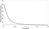 |
Fig. 1. Average percentage of pixels above threshold in calcium K line synoptic maps (solid line) as a function of threshold. Dashed line indicates the average percentage of pixels in NSO/KP synoptic maps of the photospheric magnetic field above a threshold of 50 G (3.6%). |
While the total number of pixels above the thresholds in the two data sets is the same, only 59% of pixels above the threshold in the maps of the magnetic field are also above the threshold in the calcium K line maps. The rest do not align perfectly and are in slightly different positions in the two data sets due to differences in locations and structures of photospheric active regions and chromospheric plages. We note that areas with a strong magnetic field align better than areas of weaker magnetic fields, and 67% of the total unsigned flux in pixels above the threshold in the maps of the magnetic field is located in pixels that are also above the threshold in the calcium K line maps. Also, if we count only pixels with an unsigned magnetic field above 150 G, 82% of them are above the threshold in the calcium K line maps.
While the calcium K line maps give us the locations of plages and active regions, they do not contain information about the polarity of the magnetic field. To assign a positive or negative polarity to the pixels of the selected active regions we used observations of sunspot polarity and field strength from MWO. For every pixel above the threshold we searched for a sunspot that was observed within five days of the time when the pixel crossed the central meridian, and was located within a distance of five degrees in both longitude and latitude. This distance was defined to be the distance from the center of the sunspot to the pixel, minus the radius of the sunspot, which was computed from the sunspot area under the assumption that the sunspot is circular. The observations used in the construction of the calcium K line synoptic maps are usually from near the central meridian. In situations where sunspot polarity measurements are not available for the day a calcium K line observation was made, sunspot drawings from days before and after the calcium K line observation can be used. The ten-day window is roughly the period of time a sunspot related to a plage would be visible and far enough from the limb to be reliably observed. The distance limits were chosen so that they are small compared to the typical distance between active regions, ensuring that the sunspot used to define the polarity of a pixel belongs to the same active region as the pixel itself. If one or more sunspots fulfilling these criteria were found, the pixel was given the polarity of the closest sunspot. In the resulting synoptic map the active pixels around sunspots with a negative polarity have a negative polarity, and the active pixels around sunspots with a positive polarity have a positive polarity, creating bipolar active regions. If in a connected region – connected meaning that the sides or corners of pixels touch each other – the polarity of at least ten pixels was determined, and those pixels accounted for at least a half of the total area of the connected region, nearest-neighbor interpolation was used to define the polarities of the remaining pixels and fill the region with polarity information. This essentially spreads the polarity information from the sunspots, which usually reside at the center of an active region, to the edges of the region. If we could not find the polarity of at least half of the pixels in a connected region, the whole region was discarded.
When comparing the polarities obtained for the active pixels from sunspot magnetic field information with the NSO/KP magnetic synoptic maps, we found 61% of the pixels had the correct polarity, 19% had incorrect polarity, and 20% had no polarity information. If we weighted the pixels with the observed intensity of the magnetic field, the ratios became 74%, 14%, and 12%, respectively. This means that the polarity information is more accurate in areas of strong magnetic field, like the centers of large active regions. These are the most important areas for the SFT simulation. The pixels left without polarity information on the other hand, tend to belong to weak active regions, which may not contain sunspots. It should be noted that here all pixels in discarded active regions were counted as not having polarity information, even if some of the individual pixels did have polarity information. Some of this disagreement between polarities could be a result of uncertainty in sunspot positions and observation times recorded on the sunspot drawings. Pevtsov et al. (2019) estimated that on average the heliographic coordinates of sunspots could have an uncertainty of about 0.5°.
To construct active regions from the synoptic maps of active pixels we combined the synoptic maps into one long continuous map spanning the whole studied time period. We ran a window four pixels wide in both longitude and latitude through the map, and connected all active pixels that fit inside the window. We then defined all connected active pixels as belonging to the same active region. This means that not all pixels in the final active region are necessarily next to each other; small gaps of a few pixels are allowed.
After the active regions were thus defined, the magnetic field inside them was determined. To approximate the total flux within each active region, we compared the area of the active regions identified from the calcium K line maps to the total unsigned flux contained within the same regions in the synoptic maps of the photospheric magnetic field. The integrated brightness of a plage correlates with the total flux of an active region, and is also proportional to the size of the plage, allowing us to make a linear fit between the plage area and its total flux (Pevtsov et al. 2016). The related scatter plot and fit are shown in Fig. 2. Because in an even sine-latitude grid every pixel has the same area, the total unsigned flux Φ of an active region obtained from Fig. 2 is:
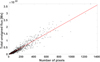 |
Fig. 2. Total unsigned flux inside a plage (in Maxwells) as a function of plage area (in number of pixels). The solid red line gives the linear fit. Data from all Carrington rotations for 1974−1985 were used. |
 (7)
(7)
where Np is the number of pixels in the active region, and Ap is the area of a single pixel. If the number of pixels of the active region is so small that the total unsigned flux becomes negative, the region is discarded. This effectively sets a lower limit of 14 pixels to the area of an active region.
The distribution of flux within each reconstructed active region is taken to be the same as the intensity distribution of calcium K line intensity within that region. This may differ from the distribution of magnetic flux in the photosphere but, as was shown in Virtanen et al. (2017), the exact distribution of flux within an active region is not important for the simulation, as long as the total flux and polarity are preserved. Using the active regions with the magnetic fluxes assigned to the pixels, we then normalized the total unsigned flux to match the value given by Eq. (7). To maintain flux balance the normalization was performed separately for positive and negative polarities, so that there are equal amounts of positive and negative flux inside each active region. This also causes the flux distributions to slightly differ from the calcium K line intensity distribution for positive and negative pixels. If the imbalance of positive and negative pixels was at least half of the total area of the region, meaning that there were at least three times as many positive pixels as negative, or vice versa, the whole active region was discarded.
We used the reconstructed active regions for the first simulation run, obtaining a set of simulated synoptic maps of the photospheric magnetic field for the studied time period. If a newly observed plage is above an already existing active region, its magnetic field is likely to have the same polarity as the active region. Because of this we can use the simulated synoptic maps to improve the accuracy of polarity information in the reconstructed active regions. We went through all active pixels for which we were unable to determine a polarity from the sunspot observations, and assigned them the polarity existing in the simulation, if the simulated field strength was at least 10 G during the rotation where the active pixel emerged, or during the previous rotation. At this step we wanted to include as much of the dissipating active regions as possible, which is why a relatively low threshold of 10 G was used. This is still clearly above the strength of the background field, but does not exclude older weakened active regions. This resulted in 67% of the pixels having the correct polarity, 22% having incorrect polarity, and 11% having no polarity information. Weighting the pixels with the intensity of the observed field, the ratios are 78%, 16%, and 6%, respectively. These numbers show a slight improvement over the original values.
To separate the effects caused by the calcium K line maps and the sunspot observations, we also created a set of active regions that use the areas and total fluxes reconstructed from calcium K line observations, but magnetogram polarities. We call this data set the area reconstruction, and it was constructed the same way as the fully reconstructed data set of active regions, except that their polarities were determined from the NSO/KP synoptic maps of the observed magnetic field. For rotations lacking observations from NSO/KP, synoptic maps of the magnetic field from MWO were used instead. It should be noted that changing the polarity of a pixel will usually also change its intensity. Because flux balance is maintained for each active region, the ratio of negative and positive pixels affects how the total flux of the region is distributed. Increasing the area covered by negative or positive polarity will therefore decrease the intensity of the field of that polarity, and vice versa.
The full reconstruction (calcium K line based areas and field strengths and sunspot polarities) includes 1193 active regions, compared to 1225 active regions identified purely from the magnetic field observations, and 1350 active regions in the area reconstruction (calcium K line based areas and field strengths, but polarities observed at NSO/KP). More active regions were identified from the calcium K line maps than from the magnetic field maps, but some were excluded in the full reconstruction due to their lack of connected sunspots to determine polarities.
Figure 3 shows Carrington rotation 1708 as an example of the true and reconstructed synoptic maps of the magnetic field. This rotation started in May 1981, near the maximum of cycle 21, and contains many sizeable active regions. On the left we can see the synoptic map of the photospheric magnetic field observed at NSO/KP (upper panel), and the active regions identified from it with a threshold of 50 G (lower panel; for a more detailed description of the identification process, see Virtanen et al. 2017). On the right is a synoptic map of calcium K line intensity (upper panel), and the active regions reconstructed from it using sunspot polarity information (lower panel). There are four large active regions in the northern hemisphere, which are all included in the full reconstruction. The polarity structures of the reconstructed regions are very similar, although not identical, to those seen in the observations. Large active regions produce a large number of sunspots, which enables us to determine polarities with fairly good accuracy even though the structure of a region could be quite complex. Many of the smaller regions on the other hand are not captured in the reconstruction due to missing polarity information. Small regions appear often without connected sunspots, which prevents us from determining polarities.
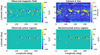 |
Fig. 3. Synoptic map of the photospheric magnetic field of Carrington Rotation 1708 (May 1981) observed at NSO/KP (top left), synoptic map of the calcium K line intensity of the same rotation (top right), active regions identified from the synoptic map of the magnetic field (bottom left), and active regions reconstructed from the calcium K line and sunspot observations (bottom right). |
5. Axial dipole moment
The axial dipole moment of the emerging active regions is one of the most important quantities for an SFT simulation. The strength of the total axial dipole of the Sun, which is strongly connected to the evolution of the polar fields, depends on the amount of axial dipole moment of the active regions inserted into the simulation. The axial dipole moment Di of an active region is defined as
 (8)
(8)
where Br is the radial magnetic field, θ is colatitude, ϕ is longitude, t is time, and integration is performed over the solid angle Ω (Wang & Sheeley 1991).
Figure 4 shows the total axial dipole moment of each Carrington rotation obtained by summing up the axial dipole moments of the individual active regions of the rotation for the active regions obtained from the NSO/KP maps, the full reconstruction, and the area reconstruction. The three curves shown in Fig. 4 exhibit a fairly similar temporal evolution, although the axial dipole moments of some individual rotations may differ. For example, the negative peaks in late 1979 and mid-1981 are clearly visible in all three, but they are stronger in the two reconstructed data sets than in the observations. The solar cycle behavior is clearly visible in all three cases, with the axial dipole moment of cycle 21 being primarily negative, as expected. The total sum of signed axial dipole moments of all observed active regions over the time depicted in Fig. 4 is −6.1 G, of all fully reconstructed active regions −6.8 G, and of all area reconstructed active regions −7.2 G. Therefore, both reconstructed data sets are within 20% of the observed value.
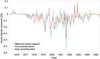 |
Fig. 4. Total axial dipole moment of the observed active regions (solid red line), the area reconstruction (dotted green line), and the fully reconstructed active regions (dashed blue line). Values are sums over Carrington rotations. |
While the overall axial dipole moment of cycle 21 is negative, some individual active regions and even Carrington rotations have a positive axial dipole moment, as can be seen in Fig. 4. The sum of the absolute values of the axial dipole moments of individual active regions is 11.9 G for the observed active regions and 13.7 G for the fully reconstructed active regions. Since in both cases the sum of signed values is roughly half of the sum of unsigned values, about 25% of axial dipole moment in both the observations and the reconstruction is positive. The ability to determine the axial dipole moment of each active region individually is one of the main advantages of this reconstruction. On the other hand, models relying on sunspot numbers and statistical properties of active regions typically assume that the polarity, tilt angle, and consequently the axial dipole moment of all active regions follows the theoretically expected axial dipole moment of the cycle.
Figure 4 does not show any systematic differences between the three curves. Instead, the differences appear to be random, the dipole moment of one series being sometimes higher and sometimes lower than in the two other series. This is important because any systematic differences, due to errors in the reconstruction for example, would most likely cause the polar fields in the simulation to drift away from the observed value. Small random variations on the other hand should not affect the long-term evolution of the polar fields, since errors in opposite directions eventually cancel each other.
6. Simulated photospheric field
Figure 5 shows supersynoptic maps of the photospheric magnetic field. The three upper panels are from the three different SFT simulations and the bottom panel shows the observed NSO/KP supersynoptic map. The first panel uses the fully reconstructed active regions and the second panel uses the active regions of the area reconstruction. In the third panel, the observed active regions identified in the NSO/KP synoptic maps of the magnetic field have been used as input. Because we do not know the strength of the polar fields at the beginning of the simulation very accurately, we have started the simulations from a map that has a constant field of 2.5 G above 60° latitude, a constant field of −2.5 G below −60° latitude, and is zero between 60° and −60°. While this choice represents the global field during a solar minimum only roughly, it is a good enough approximation to serve as a starting point. As long as the starting point is the same in all three simulations, we can compare the simulations with each other even if there is some uncertainty in the initial field. Additionally, as shown in Virtanen et al. (2017), uncertainty in the initial polar field does not have an effect on the long-term evolution of polar fields; simulations with different initial polar fields converge within one solar cycle. Thus, the later years of the simulations of Fig. 5 are not strongly affected by the initial polar field.
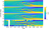 |
Fig. 5. Supersynoptic maps of the photospheric magnetic field from 1975 to 1985 from simulations using the full reconstruction (top panel), the area reconstruction (second panel from the top), and the observed active regions (third panel from the top) as input. Bottom panel: NSO/KP magnetic field observations. |
Figure 5 shows that there is somewhat less emerging flux in the simulation that uses the fully reconstructed active regions than in the two other simulations. As discussed above, some of the weaker active regions included in the simulations using the observed active regions and the area reconstruction are missing, which reduces the total flux of active regions of the full reconstruction. However, since most of these weaker regions are not strong enough to create flux surges that would reach high latitudes, they do not strongly affect the large-scale evolution of the field or the strength and development of polar fields, and the difference is only seen at low latitudes.
Most of the significant poleward surges of flux are the same in all three simulations, and they are also mostly the same as in the observations. In the northern hemisphere there are strong surges of negative flux in the late 1970s, followed by a surge of positive flux in 1980. Subsequently, new surges of negative flux appear in the early 1980s. The absolute and relative strength of the individual surges varies slightly between the three simulations. The polar field ends up being slightly stronger in the simulations using reconstructed active regions (see Fig. 6). Since the northern polar field is very similar in the simulations using active regions of the full and area reconstructions, but is weaker in the simulation using observed active regions, the differences in its strength must be caused by calcium K line plage identification, and not by sunspot polarities.
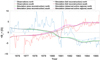 |
Fig. 6. Average magnetic field below −60° and above 60° latitude from the simulations and observations shown in Fig. 5. Dotted lines are observations, solid lines are from a simulation using the full reconstruction, dash-dotted lines are from a simulation using the area reconstruction, and dashed lines are from a simulation using the observed active regions. Blue, green, and black lines are for the northern hemisphere, while red and purple lines are for the southern hemisphere. |
In the southern hemisphere, after a number of smaller positive surges in the late 1970s, there are two major surges of positive flux, one starting in 1980 and the other in 1981−1982. These are visible in all simulations, and are mostly responsible for the development of the southern polar field of cycle 21. However, there are differences in how these two surges behave in the three simulations. In the observations they seem to be of roughly equal strength, but in the simulation using observed active regions the second surge is fairly weak. In the simulation using the area reconstruction the second surge is almost as strong as the first surge, which implies that in this case the active region identification may have worked better with the calcium K line maps than with magnetograms. In the simulation using the full reconstruction, the first surge is slightly weaker than in the other two simulations. The difference must be due to different polarity information.
Figure 6 shows the average field strength around the two poles, above 60° latitude in the north and below −60° latitude in the south according to the three simulations and the observations shown in Fig. 5. The three simulations agree with each other fairly well. In the early 1980s the southern polar field is slightly weaker in the simulation using the fully reconstructed active regions than in the other two simulations, because the first major poleward surge in 1980 is slightly weaker in this simulation (see Fig. 5). However, the difference disappears fairly quickly with the appearance of the second positive surge in 1982.
In the northern hemisphere the three simulations are very similar until 1982, when a surge of negative flux appears, which is significantly stronger in both simulations using active regions reconstructed from calcium K line observations (see also Fig. 5). During the last years the values are actually closer to the observed values in the simulations using reconstructed active regions than in the simulation using observed active regions.
The polarity reversals occur within a few months in late 1979 in all three simulations. In the observations, the final polarity reversals happen significantly later, and there are multiple reversals, which do not exist in the simulations. However, the polar fields of these early NSO/KP synoptic maps are known to suffer from errors (Harvey 2000; Harvey & Munoz-Jaramillo 2015; Virtanen & Mursula 2016). Additionally, the first years of the simulations, including the polarity reversals, are still affected by the choice of initial polar fields in 1975. The active regions start to dominate the evolution of the polar fields only close to the maximum of the cycle, when significant amounts of new flux reach high latitudes. For these reasons neither the polar fields in the ascending phase of the cycle nor the field reversal times can be confidently compared between observations and simulations. Values of the polar fields in the declining phase of the cycle and in the next minimum are much more reliable measures of the quality of the reconstruction than at earlier times. There, the agreement is very good in both hemispheres.
7. Discussion and conclusions
In this paper we study the possibility of using plages identified from calcium K line observations together with polarities determined from sunspot polarity measurements to reconstruct magnetic active regions to be used as input in a surface flux transport simulation. Using the reconstructed active regions, the SFT simulation creates complete synoptic maps of the photospheric magnetic field that allow us to study the evolution of the large-scale magnetic field, especially the polar fields. In this study we have limited ourselves to the time period from 1975 to 1985 (roughly solar cycle 21), for which synoptic maps of both the calcium K line and the photospheric magnetic field exist, allowing us to test and validate the reconstruction.
There are a few sources of uncertainty in the reconstruction process. Defining the plage areas (active regions) from the MWO calcium K line observations, determining the total flux contained in each area, and finding the correct magnetic polarity within each area can all produce uncertainties and errors in the reconstructed active regions, and consequently in the simulation. The polarity was found to be correct in roughly 70% of the pixels, but accuracy is better in large active regions with strong magnetic fields, which are the most important factor for the simulation. The axial dipole moment, which is a very important indicator of how the regions will affect polar fields in the simulation, is very similar for the reconstructed active regions and the observed active regions. The variable strength and sign of the axial dipole moment is very well captured by the reconstruction. This is a significant advantage for this reconstruction method compared to earlier methods that may only contain theoretically assumed polarity information, which is applied to all individual active regions. The identification of plages from calcium K line maps and the determination of polarities cause errors. These errors are however random in nature, and are likely to smooth out in the simulation as long as the long-term evolution of the total axial dipole moment is relatively accurate.
Simulations show that the lack of a few weak active regions slightly reduces the amount of flux in the reconstructed activity belts. Individual poleward surges of flux are slightly affected by uncertainties in plage identification or polarity determination. In both hemispheres the polar field is slightly stronger at the end of the simulation (in the late declining phase of cycle 21) with the reconstruction than with the observed active regions because of differences in plage identification. In the southern hemisphere, the polar field of the full reconstruction grows slightly more slowly, being weaker than others for a few years in the early 1980s. This is most likely due to problems in sunspot polarity determination. However, these differences are small compared to the field evolution over the solar cycle. We also note that by the end of the simulation the polar field strengths of the two reconstructions agree better with the observations than the simulation using active regions identified from the NSO/KP maps of the magnetic field.
In conclusion, we find that we are able to reconstruct the long-term evolution of the large-scale magnetic field and the polar fields with good accuracy using calcium K line-based active regions and sunspot polarity observations. While individual, mainly rather weak active regions may be missing or erroneous in the reconstruction, the randomness of the errors and the lack of long-term memory in the simulation ensure that the simulated large-scale field pattern and polar fields remain close to the values obtained from observations and may even be more reliable than simulations using active regions determined from magnetic field observations. However, there are some limitations to the use of such a reconstruction. Since there is considerable uncertainty in the structure of individual active regions, and even in the strength of individual poleward surges, the method is mainly useful for studying the long-term evolution of large-scale solar magnetic fields, including the polar fields. On short timescales the inaccuracies related to the reconstructed active regions play a more significant role.
Sunspot drawings: ftp://howard.astro.ucla.edu/pub/obs/drawings/ Carrington maps of magnetic fields: https://www.nso.edu/data/historical-archive/
Acknowledgments
We acknowledge the financial support by the Academy of Finland to the ReSoLVE Centre of Excellence (project no. 307411). The National Solar Observatory (NSO) is operated by the Association of Universities for Research in Astronomy, AURA Inc under cooperative agreement with the National Science Foundation (NSF).The data used in this work were produced in the framework of the NSO synoptic program. This study includes data from the synoptic program at the 150-Foot Solar Tower of the Mt. Wilson Observatory. The Mt. Wilson 150-Foot Solar Tower is operated by UCLA, with funding from NASA, ONR and NSF, under agreement with the Mt. Wilson Institute. Digitization of sunspot drawings was partially supported by NASA NNX15AE95G grant. This work was partially supported by the International Space Science Institute (Bern, Switzerland) via International Team 420 on Reconstructing Solar and Heliospheric Magnetic Field Evolution over the Past Century.
References
- Babcock, H. W. 1953, ApJ, 118, 387 [Google Scholar]
- Babcock, H. W., & Babcock, H. D. 1955, ApJ, 121, 349 [Google Scholar]
- Baumann, I., Schmitt, D., Schüssler, M., & Solanki, S. K. 2004, A&A, 426, 1075 [NASA ADS] [CrossRef] [EDP Sciences] [Google Scholar]
- Baumann, I., Schmitt, D., & Schüssler, M. 2006, A&A, 446, 307 [NASA ADS] [CrossRef] [EDP Sciences] [Google Scholar]
- Ellerman, F. 1919, PASP, 31, 16 [NASA ADS] [CrossRef] [Google Scholar]
- Hale, G. E. 1908, ApJ, 28, 244 [NASA ADS] [CrossRef] [Google Scholar]
- Hale, G. E., Ellerman, F., Nicholson, S. B., & Joy, A. H. 1919, ApJ, 49, 153 [NASA ADS] [CrossRef] [Google Scholar]
- Harvey, J. 2000, Kitt Peak Synoptic Data Documentation, ftp://vso.nso.edu/kpvt/synoptic [Google Scholar]
- Harvey, J., & Munoz-Jaramillo, A. 2015, AAS/AGU Triennial Earth-Sun Summit, 1, 11102 [Google Scholar]
- Howard, R. 1974, Sol. Phys., 38, 283 [NASA ADS] [CrossRef] [Google Scholar]
- Jiang, J., Cameron, R., Schmitt, D., & Schüssler, M. 2010, ApJ, 709, 301 [NASA ADS] [CrossRef] [Google Scholar]
- Jiang, J., Cameron, R. H., Schmitt, D., & Schüssler, M. 2011, A&A, 528, A82 [NASA ADS] [CrossRef] [EDP Sciences] [Google Scholar]
- Leighton, R. B. 1959, ApJ, 130, 366 [NASA ADS] [CrossRef] [Google Scholar]
- Livingston, W. C., Harvey, J., Slaughter, C., & Trumbo, D. 1976, Appl. Opt., 15, 40 [NASA ADS] [CrossRef] [Google Scholar]
- Pevtsov, A. A., Virtanen, I., Mursula, K., Tlatov, A., & Bertello, L. 2016, A&A, 585, A40 [NASA ADS] [CrossRef] [EDP Sciences] [Google Scholar]
- Pevtsov, A. A., Tlatova, K. A., Pevtsov, A. A., et al. 2019, A&A, submitted [Google Scholar]
- Tlatov, A. G., Tlatova, K. A., Vasil’eva, V. V., Pevtsov, A. A., & Mursula, K. 2015, Adv. Space Res., 55, 835 [Google Scholar]
- Virtanen, I., & Mursula, K. 2016, A&A, 591, A78 [NASA ADS] [CrossRef] [EDP Sciences] [Google Scholar]
- Virtanen, I. O. I., Virtanen, I. I., Pevtsov, A. A., Yeates, A., & Mursula, K. 2017, A&A, 604, A8 [NASA ADS] [CrossRef] [EDP Sciences] [Google Scholar]
- Virtanen, I. O. I., Virtanen, I. I., Pevtsov, A. A., & Mursula, K. 2018, A&A, 616, A134 [NASA ADS] [CrossRef] [EDP Sciences] [Google Scholar]
- Wang, Y.-M., & Sheeley, Jr., N. R. 1991, ApJ, 375, 761 [NASA ADS] [CrossRef] [Google Scholar]
- Whitbread, T., Yeates, A. R., Muñoz-Jaramillo, A., & Petrie, G. J. D. 2017, A&A, 607, A76 [NASA ADS] [CrossRef] [EDP Sciences] [Google Scholar]
- Whitbread, T., Yeates, A. R., & Muñoz-Jaramillo, A. 2018, ApJ, 863, 116 [NASA ADS] [CrossRef] [Google Scholar]
- Yeates, A. R., Baker, D., & van Driel-Gesztelyi, L. 2015, Sol. Phys., 290, 3189 [NASA ADS] [CrossRef] [Google Scholar]
All Figures
|
Fig. 1. Average percentage of pixels above threshold in calcium K line synoptic maps (solid line) as a function of threshold. Dashed line indicates the average percentage of pixels in NSO/KP synoptic maps of the photospheric magnetic field above a threshold of 50 G (3.6%). |
| In the text | |
|
Fig. 2. Total unsigned flux inside a plage (in Maxwells) as a function of plage area (in number of pixels). The solid red line gives the linear fit. Data from all Carrington rotations for 1974−1985 were used. |
| In the text | |
|
Fig. 3. Synoptic map of the photospheric magnetic field of Carrington Rotation 1708 (May 1981) observed at NSO/KP (top left), synoptic map of the calcium K line intensity of the same rotation (top right), active regions identified from the synoptic map of the magnetic field (bottom left), and active regions reconstructed from the calcium K line and sunspot observations (bottom right). |
| In the text | |
|
Fig. 4. Total axial dipole moment of the observed active regions (solid red line), the area reconstruction (dotted green line), and the fully reconstructed active regions (dashed blue line). Values are sums over Carrington rotations. |
| In the text | |
|
Fig. 5. Supersynoptic maps of the photospheric magnetic field from 1975 to 1985 from simulations using the full reconstruction (top panel), the area reconstruction (second panel from the top), and the observed active regions (third panel from the top) as input. Bottom panel: NSO/KP magnetic field observations. |
| In the text | |
|
Fig. 6. Average magnetic field below −60° and above 60° latitude from the simulations and observations shown in Fig. 5. Dotted lines are observations, solid lines are from a simulation using the full reconstruction, dash-dotted lines are from a simulation using the area reconstruction, and dashed lines are from a simulation using the observed active regions. Blue, green, and black lines are for the northern hemisphere, while red and purple lines are for the southern hemisphere. |
| In the text | |
Current usage metrics show cumulative count of Article Views (full-text article views including HTML views, PDF and ePub downloads, according to the available data) and Abstracts Views on Vision4Press platform.
Data correspond to usage on the plateform after 2015. The current usage metrics is available 48-96 hours after online publication and is updated daily on week days.
Initial download of the metrics may take a while.