| Issue |
A&A
Volume 622, February 2019
|
|
|---|---|---|
| Article Number | A156 | |
| Number of page(s) | 20 | |
| Section | Planets and planetary systems | |
| DOI | https://doi.org/10.1051/0004-6361/201834170 | |
| Published online | 15 February 2019 | |
A search for accreting young companions embedded in circumstellar disks
High-contrast Hα imaging with VLT/SPHERE★,★★
1
ETH Zurich, Institute for Particle Physics and Astrophysics,
Wolfgang-Pauli-Strasse 27,
8093
Zurich,
Switzerland
e-mail: gabriele.cugno@phys.ethz.ch
2
National Center of Competence in Research “PlanetS”,
Gesellschaftsstrasse 6,
3012
Bern,
Switzerland
3
Max-Planck-Institut für Astronomie,
Königstuhl 17,
69117
Heidelberg,
Germany
4
LESIA, CNRS, Observatoire de Paris, Université Paris Diderot,
UPMC, 5 place J. Janssen,
92190
Meudon,
France
5
Leiden Observatory, Leiden University,
PO Box 9513,
2300
RA Leiden,
The Netherlands
6
Université Grenoble Alpes, CNRS, IPAG,
38000
Grenoble,
France
7
Unidad Mixta International Franco-Chilena de Astronomía, CNRS/INSU UMI 3386 and Departemento de Astronomía, Universidad de Chile,
Casilla 36-D,
Santiago,
Chile
8
Geneva Observatory, University of Geneva,
Chemin des Mailettes 51,
1290
Versoix,
Switzerland
9
INAF – Osservatorio Astronomico di Padova,
Vicolo dell’Osservatorio 5,
35122
Padova,
Italy
10
Anton Pannekoek Astronomical Institute, University of Amsterdam,
PO Box 94249,
1090
GE Amsterdam,
The Netherlands
11
Space Telescope Science Institute,
Baltimore 21218,
MD,
USA
12
Aix-Marseille Université, CNRS, CNES, LAM,
Marseille,
France
13
Department of Astronomy, Stockholm University, AlbaNova University Center,
106 91 Stockholm,
Sweden
14
Centre de Recherche Astrophysique de Lyon, CNRS/ENSL Université Lyon 1,
9 av. Ch. André,
69561
Saint-Genis-Laval,
France
15
CNRS, IPAG,
38000
Grenoble,
France
16
The University of Michigan,
Ann Arbor,
MI
48109,
USA
17
European Southern Observatory,
Alonso de Cordova 3107, Casilla 19001 Vitacura,
Santiago 19,
Chile
18
Physikalisches Institut, Universität Bern,
Gesellschaftsstrasse 6,
3012
Bern,
Switzerland
19
Monash Centre for Astrophysics (MoCa) and School of Physics and Astronomy, Monash University,
Clayton Vic
3800,
Australia
20
NOVA Optical Infrared Instrumentation Group at ASTRON,
Oude Hoogeveensedijk 4,
7991
PD Dwingeloo,
The Netherlands
21
Institute for Computational Science, University of Zurich,
Winterthurerstrasse 190,
8057
Zurich,
Switzerland
22
Núcleo de Astronomía, Facultad de Ingeniería y Ciencias, Universidad Diego Portales,
Av. Ejercito 441,
Santiago,
Chile
23
Escuela de Ingeniería Industrial, Facultad de Ingeniería y Ciencias, Universidad Diego Portales,
Av. Ejercito 441,
Santiago,
Chile
Received:
31
August
2018
Accepted:
13
December
2018
Context. In recent years, our understanding of giant planet formation progressed substantially. There have even been detections of a few young protoplanet candidates still embedded in the circumstellar disks of their host stars. The exact physics that describes the accretion of material from the circumstellar disk onto the suspected circumplanetary disk and eventually onto the young, forming planet is still an open question.
Aims. We seek to detect and quantify observables related to accretion processes occurring locally in circumstellar disks, which could be attributed to young forming planets. We focus on objects known to host protoplanet candidates and/or disk structures thought to be the result of interactions with planets.
Methods. We analyzed observations of six young stars (age 3.5–10 Myr) and their surrounding environments with the SPHERE/ZIMPOL instrument on the Very Large Telescope (VLT) in the Hα filter (656 nm) and a nearby continuum filter (644.9 nm). We applied several point spread function (PSF) subtraction techniques to reach the highest possible contrast near the primary star, specifically investigating regions where forming companions were claimed or have been suggested based on observed disk morphology.
Results. We redetect the known accreting M-star companion HD142527 B with the highest published signal to noise to date in both Hα and the continuum. We derive new astrometry (r=62.8−2.7+2.1 mas and PA=(98.7±1.8)°) and photometry (ΔN_Ha = 6.3−0.3+0.2 mag, ΔB_Ha = 6.7 ± 0.2 mag and ΔCnt_Ha = 7.3−0.2+0.3 mag) for the companion in agreement with previous studies, and estimate its mass accretion rate (Ṁ ≈ 1−2 × 10⁻¹⁰ M⊙yr−1). A faint point-like source around HD135344 B (SAO206462) is also investigated, but a second deeper observation is required to reveal its nature. No other companions are detected. In the framework of our assumptions we estimate detection limits at the locations of companion candidates around HD100546, HD169142, and MWC 758 and calculate that processes involving Hα fluxes larger than ~ 8 × 10⁻¹⁴–10−15 erg s−1 cm−2 (Ṁ > 10−10−10−12 M⊙yr−1) can be excluded. Furthermore, flux upper limits of ~10−14−10−15 erg s−1 cm−2 (Ṁ < 10−11–10−12 M⊙yr−1) are estimated within the gaps identified in the disks surrounding HD135344 B and TW Hya. The derived luminosity limits exclude Hα signatures at levels similar to those previously detected for the accreting planet candidate LkCa15 b.
Key words: planet-disk interactions / planetary systems / techniques: high angular resolution / planets and satellites: detection
Based on observations collected at the Paranal Observatory, ESO (Chile). Program ID: 096.C-0248(B), 096.C-0267(A),096.C-0267(B), 095.C-0273(A), 095.C-0298(A).
The reduced images (FITS files) are only available at the CDS via anonymous ftp to cdsarc.u-strasbg.fr (130.79.128.5) or via http://cdsarc.u-strasbg.fr/viz-bin/qcat?J/A+A/622/A156
© ESO 2019
1 Introduction
Providing an empirical basis for gas giant planet formation models and theories requires the detection of young objects in their natal environment, i.e., when they are still embedded in the gas and dust-rich circumstellar disk surrounding their host star. The primary scientific goals of studying planet formation are as follows: to understand where gas giant planet formation takes place, for example, at what separations from the host star and under which physical and chemical conditions in the disk; how formation occurs, i.e., via the classical core accretion process (Pollack et al. 1996) or a modified version of that process (e.g., pebble accretion, Lambrechts & Johansen 2012) or direct gravitational collapse (Boss 1997); and the properties of the suspected circumplanetary disks (CPDs).
While in recent years high-contrast, high spatial resolution imaging observations of circumstellar disks have revealed an impressive diversity in circumstellar disk structure and morphology, the number of directly detected planet candidates embedded in those disks is still small (LkCa15 b, HD100546 b, HD169142 b, MWC 758 b, PDS 70 b; Kraus & Ireland 2012; Quanz et al. 2013a; Reggiani et al. 2014, 2018; Biller et al. 2014; Keppler et al. 2018). To identify these objects, high-contrast exoplanet imaging can be used. These observations are typically performed at near- to mid-infrared wavelengths using an adaptive optics-assisted high-resolution camera. In addition to the intrinsic luminosity of the still contracting young gas giant planet, the surrounding CPD, if treated as a classical accretion disk, contributes significantly to fluxes beyond 3 μm wavelength (Zhu 2015; Eisner 2015), potentially easing the detection of young forming gas giants at these wavelengths. While the majority of the forming planet candidates mentioned above were detected in this way, it has also been realized that the signature from a circumstellar disk itself can sometimes mimic that of a point source after PSF subtraction and image post-processing (e.g., Follette et al. 2017; Ligi et al. 2018). As a consequence, it is possible that some of the aforementioned candidates are false positives.
Anotherapproach is to look for direct signatures of the suspected CPDs, such as their dust continuum emission or their kinematic imprint in high-resolution molecular line data (Perez et al. 2015; Szulágyi et al. 2018). In one case, spectro-astrometry using CO line emission was used to constrain the existence and orbit of a young planet candidate (Brittain et al. 2013, 2014). Moreover, Pinte et al. (2018) and Teague et al. (2018) suggested the presence of embedded planets orbiting HD163296 from local deviations from Keplerian rotation in the protoplanetary disk. A further indirect way to inferthe existence of a young, forming planet is to search for localized differences in the gas chemistry of the circumstellar disk, as the planet provides extra energy to the chemical network in its vicinity (Cleeves et al. 2015).
Finally, it is possible to look for accretion signatures from gas falling onto the planet and its CPD. Accretion shocks are able to excite or ionize the hydrogen atoms, which then radiate recombination emission lines, such as Hα, when returning to lower energy states (e.g., Calvet & Gullbring 1998; Szulágyi & Mordasini 2017; Marleau et al. 2017). High-contrast imaging using Hα filters was already successfully applied in three cases. Using angular spectral differential imaging (ASDI) with the Magellan Adaptive Optics System (MagAO), Close et al. (2014a) detected Hα excess emission from the M-star companion orbiting the Herbig Ae/Be star HD142527, and Sallum et al. (2015) also used MagAO to identify at least one accreting companion candidate located in the gap of the transition disk around LkCa15. The accretion signature was found at a position very similar to the predicted orbital position of one of the faint point sources detected by Kraus & Ireland (2012), attributed to a forming planetary system. Most recently, Wagner et al. (2018) have claimed the detection of Hα emission from the young planet PDS70 b using MagAO, albeit with comparatively low statistical significance (3.9σ).
In this paper we present aset of Hα high-contrast imaging data for six young stars, aiming at the detection of potential accretion signatures from the (suspected) young planets embedded in the circumstellar disks of the stars. The paper is structured as follows: in Sect. 2 we discuss the observations and target stars. We explain the data reduction in Sect. 3 and present our analyses in Sect. 4. In Sect. 5 we discuss our results in a broader context and conclude in Sect. 6.
2 Observations and target sample
2.1 Observations
The data were all obtained with the ZIMPOL sub-instrument of the adaptive optics (AO) assisted high-contrast imager SPHERE (Beuzit et al. 2008; Petit et al. 2008; Fusco et al. 2016), which is installed at the Very Large Telescope (VLT) of the European Southern Observatory (ESO) on Paranal in Chile. A detailed description of ZIMPOL can be found in Schmid et al. (2018). Some of the data were collected within the context of the Guaranteed Time Observations (GTO) program of the SPHERE consortium; others were obtained in other programs and downloaded from the ESO data archive(program IDs are listed in Table 1). We focused on objects that are known from other observations to host forming planet candidates that still need to be confirmed (HD100546, HD169142, and MWC 758)1, objects known to host accreting stellar companions (HD142527), and objects that have well-studied circumstellar disks with spatially resolved substructures (gaps, cavities, or spiral arms), possibly suggesting planet formation activities (HD135344 B and TW Hya). All data were taken in the noncoronagraphic imaging mode of ZIMPOL using an Hα filter in one camera arm and a nearby continuum filter simultaneously in the other arm (Cont_Ha; λc = 644.9 nm, Δλ = 3.83 nm). As the data were observed in different programs, we sometimes used the narrow Hα filter (N_Ha; λc = 656.53 nm, Δλ = 0.75 nm) and sometimes the broad Hα filter (B_Ha; λc = 655.6 nm, Δλ = 5.35 nm). A more complete description of these filters can be found in Schmid et al. (2017). To establish which filter allows for the highest contrast performance, we used HD142527 and its accreting companion (Close et al. 2014a) as a test target and switched between the N_Ha and the B_Ha filter every ten frames within the same observing sequence. All datasets were observed in pupil-stabilized mode to enable angular differential imaging (ADI; Marois et al. 2006). The fundamental properties of the target stars are given in Table 2, while a summary of the datasets is given in Table 1.
We notethat because of the intrinsic properties of the polarization beam splitter used by ZIMPOL, polarized light might preferentially end up in one of the two arms, causing a systematic uncertainty in the relative photometry between the continuum and Hα frames. The inclined mirrors in the telescope and the instrument introduce di-attenuation (e.g., higher reflectivity for I⊥ than I∥) and polarization cross talks, so that the transmissions in imaging mode to the I⊥ and I∥ arm depend on the telescope pointing direction. This effect is at the level of a few percent (about ± 5%), but unfortunately the dependence on the instrument configuration has not been determined yet. We discuss its potential impact on our analyses in Appendix A, even though we did not take this effect into account since it is small and could not be precisely quantified.
2.2 Target sample
2.2.1 HD142527
HD142527 is known to have a prominent circumstellar disk (e.g., Fukagawa et al. 2006; Canovas et al. 2013; Avenhaus et al. 2014b) and a close-in M star companion (HD142527 B; Biller et al. 2012; Rodigas et al. 2014; Lacour et al. 2016; Christiaens et al. 2018; Claudi et al. 2019) that shows signatures of ongoing accretion in Hα emission (Close et al. 2014a). This companion orbits in a large, optically thin cavity within the circumstellar disk stretching from ~ 0′′. 07 to ~ 1′′. 0 (e.g., Fukagawa et al. 2013; Avenhaus et al. 2014b), and it is likely that this companion is at least partially responsible for clearing the gap by accretion of disk material (Biller et al. 2012; Price et al. 2018). Avenhaus et al. (2017) obtained polarimetric differential imaging data with SPHERE/ZIMPOL in the very broad band (VBB, as defined in Schmid et al. 2018) optical filter, revealing new substructures, and resolving the innermost regions of the disk (down to 0′′.025). In addition, extended polarized emission was detected at the position of HD142527 B, possibly due to dust in a circumsecondary disk. Christiaens et al. (2018) extracted a medium-resolution spectrum of the companion and suggested a mass of 0.34 ± 0.06 M⊙. This value is a factor of~3 larger than that estimated by spectral energy distribution (SED) fitting (Lacour et al. 2016, M = 0.13 ± 0.03 M⊙). Thanks to the accreting close-in companion, this system is the ideal target to optimize the Hα observing strategy with SPHERE/ZIMPOL and also the data reduction.
Summary of observations.
2.2.2 HD135344 B
HD135344 B (SAO206462) is surrounded by a transition disk that was spatially resolved at various wavelengths. Continuum (sub-)millimeter images presented by Andrews et al. (2011) and van der Marel et al. (2016) revealed a disk cavity with an outer radius of 0′′.32. In polarimetric differential imaging (PDI) observations in the near-infrared (NIR), the outer radius of the cavity appears to be at 0′′. 18, and the difference in apparent size was interpreted as a potential indication for a companion orbiting in the cavity (Garufi et al. 2013). Data obtained in PDI mode also revealed two prominent, symmetric spiral arms (Muto et al. 2012; Garufi et al. 2013; Stolker et al. 2016). Vicente et al. (2011) and Maire et al. (2017) searched for planets in the system using NIR NACO and SPHERE high-contrast imaging data, but did not find any. Using hot start evolutionarymodels these authors derived upper limits for the mass of potential giant planets around HD135344 B (3 MJ beyond 0′′. 7).
2.2.3 TW Hya
TW Hya is the nearest T Tauri star to Earth. Its almost face-on transitional disk (i ~ 7 ± 1°; Qi et al. 2004) shows multiple rings and gaps in both dust continuum and scattered light data. Hubble Space Telescope (HST) scattered light images from Debes et al. (2013) first allowed the identification of a gap at ~ 1′′. 48. Later, Akiyama et al. (2015) observed in H-band polarized images a gap at a separation of ~0′′.41. Using Atacama Large Millimeter Array (ALMA), Andrews et al. (2016) identified gaps from the radial profile of the 870 μm continuum emission at 0′′.41, 0′′. 68 and 0′′. 80. Finally, van Boekel et al. (2017) obtained SPHERE images in PDI and ADI modes at optical and NIR wavelengths, and identified three gaps at 0′′.11, 0′′. 39, and 1′′. 57 from the central star. A clear gap was also identified by Rapson et al. (2015) at a separation of 0′′. 43 in Gemini/GPI polarimetric images and the largest gap at r ≃ 1′′.52 has also been observed in CO emission with ALMA (Huang et al. 2018).
2.2.4 HD100546
The disk around HD100546 was also spatially resolved in scattered light and dust continuum emission in different bands (e.g., Augereau et al. 2001; Quanz et al. 2011; Avenhaus et al. 2014a; Walsh et al. 2014; Pineda et al. 2014). The disk appears to be almost, but not completely, devoid of dusty material at radii between a few and 13 AU. This gap could be due to the interaction with a young forming planet, and Brittain et al. (2013, 2014) suggested the presence of a companion orbiting the star at 0′′. 13, based on high-resolution NIR spectro-astrometry of CO emission lines. Another protoplanet candidate was claimed by Quanz et al. (2013a) using L′ band high-contrast imaging data. The object was found at 0′′.48 ± 0′′.04 from the central star, at a position angle (PA) of  , with an apparent magnitude of L′ = 13.2 ± 0.4 mag. Quanz et al. (2015) reobserved HD100546 in different bands (L′, M′, Ks) and detected theobject again in the first two filters. Based on the colors and observed morphology these authors suggested that the data are best explained by a forming planet surrounded by a circumplanetary disk. Later, Currie et al. (2015) recovered HD100546 b from H-band integral field spectroscopy (IFS) with the Gemini Planet Imager (GPI; Macintosh et al. 2006) and identified a second putative point source c closer to the star (rproj ~ 0′′.14) potentially related to the candidate identified by Brittain et al. (2013, 2014). More recently, Rameau et al. (2017) demonstrated that the emission related to HD100546 b appears to be stationary and its spectrum is inconsistent with any type of low temperature objects. Furthermore, they obtained Hα images withthe MagAO instrument to search for accretion signatures, but no point source was detected at either the b or c position, and they placed upper limits on the accretion luminosity (Lacc < 1.7 × 10⁻⁴ L⊙). The same data were analyzed by Follette et al. (2017), together with other Hα images (MagAO), H band spectra (GPI), and Y band polarimetric images (GPI). Their data exclude that HD100546 c is emitting in Hα with LHα > 1.57 × 10⁻⁴L⊙.
2.2.5 HD169142
HD169142 is surrounded by a nearly face-on pre-transitional disk. Using PDI images, Quanz et al. (2013b) found an unresolved disk rim at 0′′. 17 and an annular gap between 0′′.28 and 0′′.49. These results were confirmed by Osorio et al. (2014), who investigated the thermal emission (λ = 7 mm) of large dust grains in the HD169142 disk, identifying two annular cavities (~ 0′′.16 − 0′′.21 and ~ 0′′.28 − 0′′.48). The latter authors also identified a point source candidate in the middle of the outer cavity at a distance of 0′′. 34 and PA ~ 175°. Biller et al. (2014) and Reggiani et al. (2014) observed a point-like feature in NaCo L′ data at the outer edge of the inner cavity (separation = 0′′.11–0′′.16 and PA = 0°−7.4°). Observations in other bands (H, KS, zp) with the Magellan Clay Telescope (MagAO/MCT) and with GPI in the J band failed to confirm the detection (Biller et al. 2014; Reggiani et al. 2014), but revealed another candidate point source albeit with low signal-to-noise ratio (S/N; Biller et al. 2014). In a recent paper, Ligi et al. (2018) explained the latter Biller et al. (2014) detection with a bright spot in the ring of scattered light from the disk rim, potentially following Keplerian motion. Pohl et al. (2017) and Bertrang et al. (2018) compared different disk and dust evolutionary models to SPHERE J-band and VBB PDI observations. Both works tried to reproduce and explain the complex morphological structures observed in the disk and conclude that planet-disk interaction is occurring in the system, even though there is no clearly confirmed protoplanet identified to date.
Target sample.
2.2.6 MWC 758
MWC 758 issurrounded by a pre-transitional disk (e.g., Grady et al. 2013). Andrews et al. (2011) found an inner cavity of ~ 55 AU based on dust continuum observations, which was, however, not observed in scattered light (Grady et al. 2013; Benisty et al. 2015). Nevertheless, PDI and direct imaging from the latter studies revealed two large spiral arms. A third spiral arm has been suggested based on VLT/NaCo L′ data by Reggiani et al. (2018), together with the claim of the detection of a point-like source embedded in the disk at (111 ± 4) mas. This object was observed in two separate datasets from 2015 and 2016 at comparable separations from the star, but different PAs, which was possibly due to orbital motion. The contrast of this object relative to the central star in the L′ band is ~ 7 mag, which, according to the BT-Settl atmospheric models (Allard et al. 2012), corresponds to the photospheric emission of a 41–64 MJ object for the age of the star. More recently, ALMA observations from Boehler et al. (2018) traced the large dust continuum emission from the disk. Two rings at 0′′.37 and 0′′.53 were discovered that are probably related to two clumps with large surface density of millimeter dust and a large cavity of ~ 0′′.26 in radius. Finally, Huélamo et al. (2018) observed MWC 758 in Hα with SPHERE/ZIMPOL, reaching an upper limit for the line luminosity of  (corresponding to a contrast of 7.6 mag) at the separation of the protoplanet candidate. No other point-like features were detected.
3 Data reduction
The basic data reduction steps were carried out with the ZIMPOL pipeline developed and maintained at ETH Zürich. The pipeline remapped the original 7.2 mas/pixel × 3.6 mas/pixel onto a square grid with an effective pixel scale of 3.6 mas × 3.6 mas (1024 × 1024 pixels). Afterward, the bias was subtracted and a flat-field correction was applied. We then aligned the individual images by fitting a Moffat profile to the stellar point spread functions (PSFs) and shifting the images using bilinear interpolation. The pipeline also calculated the parallactic angle for each individual frame and added the information to the image header. Finally, we split up the image stacks into individual frames and grouped them together according to their filter, resulting in two image stacks for each object: one for an Hα filter and one for the continuum filter2. In general, all images were included in the analysis if not specifically mentioned in the individual subsections. The images in these stacks were cropped to a size of 1′′.08 × 1′′.08 centered on the star. This allowed us to focus our PSF subtraction efforts on the contrast dominated regime of the images. The removal of the stellar PSF was performed in three different ways: ADI, spectral differential imaging (SDI), and ASDI (a two-step combination of SDI and ADI).
To perform ADI, we fed the stacks into our PynPoint pipeline (Amara & Quanz 2012; Amara et al. 2015; Stolker et al. 2019). The PynPoint package uses principal component analysis (PCA) to model and subtract the stellar PSF in all individual images before they are derotated to a common field orientation and mean-combined. To investigate the impact on the final contrast performance for all objects, we varied the number of principal components (PCs) used to fit the stellar PSF and the size of the inner mask that is used to cover the central core of the stellar PSF prior to the PCA. No frame selection based on the field rotation was applied, meaning that all the images were considered for the analysis, regardless of the difference in parallactic angle. The SDI approach aims at reducing the stellar PSF using the fact that all features arising from the parent star (such as Airy pattern and speckles) scale spatially with wavelength λ, while the position of a physical object on the detector is independentof λ. The underlying assumption is that, given that λc is similar in all filters, the continuum flux density is the same at all wavelengths. To this end, modified versions of the continuum images were created. First, they were multiplied with the ratio of the effective filter widths to normalize the throughput of the continuum filter relative to the Hα filter3. Then, they were spatially stretched using spline interpolation in radial direction, going out from the image center, by the ratio of the central wavelengths of the filters to align the speckle patterns. Because of the possibly different SED shapes of our objects with respectto the standard calibration star used in Schmid et al. (2017) to determine the central wavelengths λc of the filters, it is possible that λc is slightly shifted for each object. This effect, however, is expected to alter the upscaling factor by at most 0.4% for B_Ha (assuming the unrealistic case in which λc is at the edge of the filter), which is the broadest filter we used. This is negligible at very small separations from the star, where speckles dominate the noise. Values for filter central wavelengths and filter equivalent widths can be found in Table 5 of Schmid et al. (2017). The modified continuum images were then subtracted from the images taken simultaneously with the Hα filter, leaving only Hα line flux emitted from the primary star and potential companions. As a final step, the images resulting from the subtraction are derotated to a common field orientation and mean-combined. It is worth noting that if, as a result of the stretching, a potential point-source emitting a significant amount of continuum flux moves by more than λ∕D, the signal strength in the Hα image is only marginally changed in the SDI subtraction step, and only the speckle noise is reduced. If this is not the case, this subtraction step yields asignificant reduction of the source signal in addition to the reduction of the speckle noise. For SPHERE/ZIMPOL Hα imaging, a conservative SDI subtraction without substantial signal removal is achieved for angular separations ≳ 0′′.90 (~ 250 pixels). Nevertheless, this technique is expected to enhance the S/N of accreting planetary companions even at smaller separations, since young planets are not expected to emit a considerable amount of optical radiation in the continuum. In this case, the absence of a continuum signal guarantees that the image subtraction leaves the Hα signal of the companion unchanged and only reduces the speckle residuals. Therefore, for this science case, there is no penalty for using SDI.
To perform ASDI, the SDI (Hα-Cnt_Hα) subtracted images are fed into the PCA pipeline to subtract any remaining residuals. During the analysis we varied the same parameters as described for simple ADI. The HD142527 dataset was used to compare the different sensitivities achieved when applying ADI, SDI, and ASDI. The results are discussed in Sect. 4.1.1 and Appendix B.
With ZIMPOL in imaging mode, there is a constant offset of  between the parallactic angle and the PA of the camera in sky coordinates (Maire et al. 2016). A preliminary astrometric calibration showed, however, that this reference frame has to be rotated by
  to align images with north pointing to the top (Ginski et al., in prep.). This means that overall, for every PSF subtraction technique, the final images have to be rotated by
  in the counterclockwise direction.
4 Analysis and results
4.1 HD142527 B: the accreting M-star companion
4.1.1 Comparing the performance of multiple observational setups
In this section, we quantitatively compare the detection performance for multiple filter combinations and PSF subtraction techniques and establish the best strategy for future high-contrast Hα observationswith SPHERE/ZIMPOL. For the analysis, the HD142527 dataset was used; during the data reduction, no further frame selection was applied. The final images of HD142527 clearly show the presence of the M-star companion east of the central star. The signal is detected in all filters with ADI (B_Ha, N_Ha, and Cnt_Ha) and ASDI (in both continuum-subtracted B_Ha and N_Ha images) over a broad range of PCs and also for different image and inner mask sizes (see Fig. 1).
We used the prescription from Mawet et al. (2014) to compute the false positive fraction (FPF) as a metric to quantify the confidence in the detection. The flux is measured in apertures of diameter λ∕D (16.5 mas) at the position of the signal and in equally spaced reference apertures placed at the same separation but with different PAs, so thatthere is no overlap between these angles and the remaining azimuthal space is filled. These apertures sample the noise at the separation of the companion. Since the apertures closest to the signal are dominated by negative wings from the PSF subtraction process, they were ignored. Then, we used Eqs. (9) and (10) from Mawet et al. (2014) to calculate S/N and FPF from these apertures. This calculation takes into account the small number of apertures that sample the noise and uses the Student t-distribution to calculate the confidence of a detection. The wider wings of the t-distribution enable a better match to a non-Gaussian residual speckle noise than the normal distribution. However, the true FPF values could be higher if the wings of the true noise distribution are higher than those of the t-distribution4.
The narrow N_Ha filter delivers a significantly lower FPF than the broader B_Ha filter over a wide range of PCs (see Fig. B.1). Figure B.1 also shows that the combination of SDI and ADI yields lower FPF values than only ADI for both filters. Applying ASDI on N_Ha images is hence the preferred choice for future high-contrast imaging programs with SPHERE/ZIMPOL in the speckle-limited regime close to the star. Furthermore, as shown in Fig. C.1 and explained in Appendix C, it is crucial to plan observations maximizing the field rotation to best modulate and subtract the stellar PSF and to achieve higher sensitivities.
In Fig. 2 we show the resulting contrast curves for the three filters for a confidence level (CL) of 99.99995%. For each dataset (B_Ha, N_Ha, and Cnt_Ha) and technique (ADI and ASDI), we calculated the contrast curves for different numbers of PCs (between 10 and 30 in steps of 5) after removing the companion (see Sect. 4.1.2). From each set of curves, we only considered the best achievable contrast at each separation from the central star. The presence of Hα line emission from the central star made SDI an inefficient technique to search for faint objects at small angular separations.
To derive the contrast curves, artificial companions with varying contrast were inserted at six different PAs (separated by 60°) and in steps of 0′′. 03 in the radial direction. As the stellar PSF was unsaturated in all individual frames, the artificial companions were obtained by shifting and flux-scaling the stellar PSFs and then adding these companions to the original frames. Also, for the calculation of the ASDI contrast curves, the original Hα filter images, containing underlying continuum and Hα line emission, were used to create artificial secondary signals. For each reduction run only one artificial companion was inserted at a time to keep the PCs as similar as possible to the original reduction. The brightness of the artificial signals was reduced/increased until their FPF corresponded to a detection with a CL of 99.99995% (i.e., a FPF of 2.5 × 10⁻⁷), corresponding to ≈5σ whether Gaussian noise was assumed. An inner mask with a radius of 0′′. 02 was used to exclude the central parts dominated by the stellar signal. The colored shaded regions around each curve represent the standard deviation of the contrast achieved at that specific separation within the six PAs.
It is important to note that, while in Fig. B.1 the N_Ha filter provides the lowest FPF for the companion, Fig. 2 seems to suggest that the B_Ha filter provides a better contrast performance. However, this is an effect from the way the contrast analysis is performed. As described above, the stellar PSF was used as a template for the artificialplanets, as it is usually done in high-contrast imaging data analysis. The flux distribution within a given filter can vary significantly depending on the object. In this specific case, HD142527 B is known to have Hα excess emission, hence the flux within either Hα filter is strongly dominated by line emission (~50% in B_Ha and ~83% in N_Ha filter) and a contribution from the optical continuum can be neglected. The primary shows, however, strong and non-negligible optical continuum emission that contributes to the flux observed in the Hα filters. Indeed, for the primary, only 10% and 56% of the flux in the B_Ha and N_Ha filters are attributable to line emission. Hence, when using the stellar PSF as template for artificial planets, we obtain a better contrast performance for the B_Ha filter as it contains overall more flux. In reality, however, if the goal is to detect Hα line emission from low-mass accreting companions, the N_Ha filter is to be preferred. Finally, as found by Sallum et al. (2015) for the planet candidate LkCa15 b, the fact that ASDI curves reach a deeper contrast confirms that this technique, in particular close to the star, is more effective and should be preferred to search for Hα accretion signals.
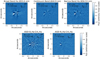 |
Fig. 1 Final ADI and ASDI reduced images of HD142527. Top row: B_Ha, Cnt_Ha, and N_Ha filter images resulting in the lowest FPFs (1.5 × 10⁻¹¹, 2.2 × 10⁻⁹, and < 10−17, corresponding to S/Ns of 13.1, 9.8, and 26.6, respectively). Bottom row: final images after ASDI reduction for B_Ha-Cnt_Ha and N_Ha-Cnt_Ha frames (4.4 × 10⁻¹⁶ and < 10−17, corresponding to S/Ns of 22.7 and 27.6). We give the number of subtracted PCs and the radius of the central mask in milliarcseconds in the top left corner of each image. The color scales are different for the two rows. Because all images of the top row have the same color stretch, the detection appears weaker in the continuum band. |
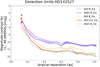 |
Fig. 2 Contrast curves for HD142527. The colored shaded regions around each curve represent the standard deviation of the achieved contrast at the 6 azimuthal positions considered at each separation. The markers (red diamond, orange circle, and violet star) represent the contrast of HD142527 B. |
4.1.2 Quantifying the Hα detection
The clear detection of the M-star companion in our images allows us to determine its contrast in all the filters and its position relative to the primary at the epoch of observation. For this purpose, we applied the Hessian matrix approach (Quanz et al. 2015) and calculated the sum of the absolute values of the determinants of Hessian matrices in the vicinity of the companion’s signal. The Hessian matrix represents the second derivative of an n-dimensional function and its determinant is a measure for the curvature of the surface described by the function. This method allows for a simultaneous determination of the position and the flux contrast of the companion and we applied a Nelder–Mead (Nelder & Mead 1965) simplex algorithm to minimize the curvature, i.e., the determinants of the Hessian matrices. We inserted negative, flux-rescaled stellar PSFs at different locations and with varying brightness in the input images and computed the resulting curvature within a region of interest (ROI) around the companion after PSF subtraction5. To reduce pixel-to-pixel variations after the PSF-subtraction step and allow for a more robust determination of the curvature, we convolved the images with a Gaussian kernel with a full width at half maximum (FWHM) of 8.3 mas (≈ 0.35 of the FWHM of the stellar PSF, which was calculated to be 23.7 mas on average). To fully include the companion’s signal, the ROI was chosen to be (43.2 × 43.2) mas around the peak flux detected in the original set of PSF subtracted images. Within the ROI, the determinants of the Hessian matrices in 10 000 evenly spaced positions on a fixed grid (every 0.43 mas) were calculated and summed up.
For the optimization algorithm to converge, we need to provide a threshold criterion: if the change in the parameters (position and contrast) between two consecutive iterations is less than a given tolerance, the algorithm has converged and the optimization returns those values for contrast and position. The absolute tolerance for the convergence was set to be 0.16, as this value is the precision to which artificial signals can be inserted into the image grid. This value applies for all the investigated parameters (position and contrast). Errors in the separation and PA measurements take into account the tolerance given for the converging algorithm and the finite grid. Errors in the contrast magnitude only consider the uncertainty due to the tolerance of the optimization. To account for systematic uncertainties in the companion’s location and contrast resulting from varying self-subtraction effects in reductions with different numbers of PCs, we ran the Hessian matrix algorithm for reductions with PCs in the range between 13 and 29 and considered the average of each parameter as final result. This range of PCs corresponds to FPF values below 2.5 × 10⁻⁷ (see Fig. B.1). To quantify the overall uncertainties in separation, PA, and contrast in a conservative way, we considered the maximum/minimum value (including measurement errors) among the set of results for the specific parameter and computed its difference from the mean. In Fig. 3, we present the results from this approach for the N_Ha dataset and show the comparison between the original residual image and the image with the companion successfully removed.
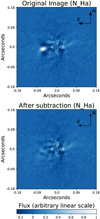 |
Fig. 3 Image of HD142527 before (top panel) and after (bottom panel) the insertion of the negative companionresulting from the Hessian matrix algorithm. The image flux scale is the same in both images. In this case 14 PCs were subtracted and a mask of 10.8 mas (radius) was applied on the 101 × 101 pixels images of the N_Ha stack. |
4.1.3 Astrometry
The previously described algorithm was used to determine the best combination of separation, PA, and magnitude contrast for HD142527 B. In the N_Ha data the companion is located at  mas from the primary star, in the B_Ha dataset at
  mas, and in the Cnt_Ha data at
  mas. The corresponding PAs are
  ,
,  and
and  , respectively.Errors in the PA measurements also take into account the above mentioned uncertainty in the astrometric calibration of the instrument, which was added in quadrature to the PA error bars.
As within the error bars all filters gave the same results, we combined them and found that HD142527 B is located at a projected separation of  mas from the primary star(
 AU at 157.3 ± 1.2 pc) and has a PA of
  . The final values result from calculating the arithmetic mean of all the values obtained from the three different datasets, while their errors are calculated identically to those for each single dataset.
In Fig. 4 we compare the positions previously estimated (Close et al. 2014a; Rodigas et al. 2014; Lacour et al. 2016; Christiaens et al. 2018) and that resulting from our analysis. Lacour et al. (2016) used a Markov chain Monte Carlo analysis to infer the orbital parameters of HD142527 B. Because the past detections were distributed over a relatively small orbital arc (~ 15°), it was difficult to constrain the parameters precisely. The high precision measurement added by our SPHERE/ZIMPOL data extends the arc to a range of ~ 30°. An updated orbital analysis is provided in Claudi et al. (2019). Figure 4 shows that HD142527 B is clearly approaching the primary in the plane of the sky.
Summary of the stellar fluxes measured in the different filters in our ZIMPOL data and the derived Hα line fluxes for our targets (last column).
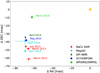 |
Fig. 4 Position of HD142527 B based on NaCo sparse aperture masking (red pentagons), MagAO (cyan triangles), GPI non-redundant masking (dark green diamonds) and VLT/SINFONI (blue circle) data from Rodigas et al. (2014), Close et al. (2014a), Lacour et al. (2016), and Christiaens et al. (2018), together with the SPHERE/ZIMPOL observation presented in this work (light green square). The position of HD142527 A is shown with the yellow star at coordinates (0,0). |
4.1.4 Photometry
The Hessian matrix approach yields the contrasts between HD142527 A and B in every filter: ΔN_Ha in the narrow band, ΔB_Ha = 6.7 ± 0.2mag in the broad band, and ΔCnt_Ha
 in the continuum filter. To quantify the brightness of the companion and not only its contrast with respect to the central star, we determined the flux of the primary in the multiple filters. We measured the count rate (cts) in the central circular region with radius ~ 1′′.5 in all frames of each stack and computed the mean and its uncertainty
  , where σ is the standard deviation of the count rate within the dataset and n is the number of frames. No aperture correction was required because the same aperture size was used by Schmid et al. (2017) to determine the zero points for the flux density for the three filters from photometric standard star calibrations. To estimate the continuum flux density we used their Eq. (4)
 (1)
(1)
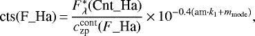
where  is the zero point of the Cnt_Ha filter, cts = 1.105 (± 0.001) × 105 ct s−1 is the count rate measured from our data, am = 1.06 is the average airmass, k1 is the atmospheric extinction at Paranal (k1(λ) = 0.085 mag/airmass for Cnt_Ha, k1(λ) = 0.082 mag/airmass for B_Ha and N_Ha; cf. Patat et al. 2011), and mmode = − 0.23 mag is the mode-dependent transmission offset, which takes into account the enhanced throughput of the R-band dichroic with respect to the standard gray beam splitter. The flux density of the primary star in the continuum filter
 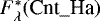 was then used to estimate the fraction of counts in the line filters due to continuum emission via
 (2)
(2)
where  is the continuum zero point of the Hα filter used in the observations (cf. Schmid et al. 2017). During this step, we assumed that the continuum flux density was the same in the three filters. The continuum count rate was subtracted from the total count rate in B_Ha and N_Ha, cts (B_Ha) = 1.631 (±0.001) × 105 ct s−1 and cts (N_Ha) = 3.903 (±0.003) × 104 ct s−1, leaving only the flux due to pure Hα emission. These were used, together with Eq. (1) with line zero points, to determine the pure Hα line fluxes (see fifth column in Table 3). For each filter, the continuum flux density was multiplied by the filter equivalent width, and the flux contribution from line emission was added for the line filters. As in Sallum et al. (2015), we assumed the B object to have the same extinction as A, ignoring additional absorption from the disk. Indeed, we considered an extinction of AV = 0.05 mag (Fairlamb et al. 2015) and, interpolating the standard reddening law of Mathis (1990) for RV = 3.1, we estimated the extinction at ~650 nm to be AHα = 0.04 mag. The stellar flux was found to be 6.1 ± 0.2 × 10⁻¹¹ erg s−1 cm−2 in the Cnt_Ha filter, 9.7 ± 0.8 × 10⁻¹¹ erg s−1 cm−2 in the B_Ha filter and 3.0 ± 0.8 × 10⁻¹¹ erg s−1 cm−2 in the N_Ha filter (see Table 3). With the empirically estimated contrasts, we calculated the companion flux, i.e., line plus continuum emission or continuum only emission, in the three filters as follows:
![\[ F^p_{{\textrm{Cnt}\_{\textrm{Ha}}}}{\,=\,}7.4^{+1.4}_{-2.1}{\,\times\,}10^{-14}{\textrm{erg}\,\textrm{s}}^{-1}\,\textrm{cm}^{-2}, \]](/articles/aa/full_html/2019/02/aa34170-18/aa34170-18-eq27.png)
![\[ F^p_ {{\textrm{B}\_{\textrm{Ha}}}}{\,=\,}2.0\,\pm\,0.4{\,\times\,}10^{-13}{{\textrm{erg}\,\textrm{s}}^{-1}\,\textrm{cm}^{-2}}, \]](/articles/aa/full_html/2019/02/aa34170-18/aa34170-18-eq28.png)
![\[ F^p_{{\textrm{N}\_{\textrm{Ha}}}}{\,=\,}9.1^{+3.5}_{-2.9}{\,\times\,}10^{-14}{\textrm{erg}\,\textrm{s}}^{-1}\,\textrm{cm}^{-2}. \]](/articles/aa/full_html/2019/02/aa34170-18/aa34170-18-eq29.png)
We notethat the contrast we calculated in the continuum filter is very similar to that obtained by Close et al. (2014a) of Δmag = 7.5 ± 0.25 mag. The direct estimation of the brightness of the primary in each individual ZIMPOL filter led to a larger difference when comparing the companion’s apparent magnitude in our work (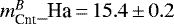 mag) with that from Close et al. (2014a;
 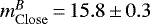 mag). Such values are possibly consistent within the typical variability of accretion of the primary and secondary at these ages. However, given the different photometry sources and filters used for the estimation of the stellar flux densities in the two works, the results cannot be easily compared.
4.1.5 Accretion rate estimates
The difference between the flux in the line filters and the continuum filter (normalized to the Hα filter widths) represents the pure Hα line emission for which we find for HD142527 B  erg s−1 cm−2 and
  erg s−1 cm−2, respectively. The line flux is then converted into a line luminosity multiplying it by the Gaia distance squared (see Table 2), yielding
  and
and  . We then estimated the accretion luminosity with the classical T Tauri stars (CTTS) relationship from Rigliaco et al. (2012), in which the logarithmic accretion luminosity grows linearly with the logarithmic Hα luminosity
 (3)
(3)
and a = 1.49 ± 0.05 and b = 2.99 ± 0.16 are empirically determined. We calculated the accretion luminosity for both datasets, yielding 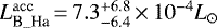 and
and 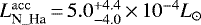 .
.
Following Gullbring et al. (1998) we finally used
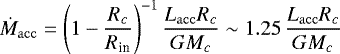 (4)
(4)
to constrain the mass accretion rate. The quantity G is the universal gravitational constant, and Rc and Mc are the radius and mass of the companion, respectively. Assuming that the truncation radius of the accretion disk Rin is ~ 5Rc, we obtain 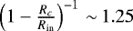 . For the companion mass and radius, two different sets of values were considered: Lacour et al. (2016) fitted the SED of HD142527 B with evolutionary models (Baraffe et al. 2003) and calculated Mc = 0.13 ± 0.03 M⊙ and Rc = 0.9 ± 0.15 R⊙, while Christiaens et al. (2018) estimated from H + K band VLT/SINFONI spectra Mc = 0.34 ± 0.06 M⊙ and Rc = 1.37 ± 0.05 R⊙, in the presence of a hot circumstellar environment7. The accretion rates obtained from the Hα emission line are
  and
and  in the first case and ṀB_Ha = 1.2 ± 1.1 × 10⁻¹⁰ M⊙ yr−1 and ṀN_Ha = 0.8 ± 0.7 × 10⁻¹⁰ M⊙∕yr in the second case. Some Hα flux loss from the instrument when the N_Ha filter is used might explain the lower value of ṀN_Ha compared to ṀB_Ha. Indeed, according to Fig. 2 and Table 5 from Schmid et al. (2017), the N_Ha filter is not perfectly centered on the Hα rest wavelength, implying that a fraction of the flux could be lost, in particular if the line profile is asymmetric. Moreover, high temperature and high velocities of infalling material cause Hα emission profiles of CTTS to be broad (Hartmann et al. 1994; White & Basri 2003). Also, line broadening from the rotation and line shift of the object due to possible radial motion might be important, even though it is not expected to justify the ~ 40% Hα flux difference of HD142527B. We argue, therefore, that with the available data it is very difficult to estimate the amount of line flux lost by the N_Ha filter, and that the value given by the B_Ha filter is expected to be more reliable, since all line emission from the accreting companion is included.
As shown in PDI images from Avenhaus et al. (2017), dust is present at the separation of the secondary possibly fully embedding the companion or in form of a circumsecondary disk. During our calculations, we neglected any local extinction effects due to disk material. It is therefore possible that on the one hand some of the intrinsic Hα flux gets absorbed/scattered and the actual mass accretion rate is higher than that estimated in this work; on the other hand, the material may also scatter someHα (or continuum) emission from the central star, possibly contributing in very small amounts to the total detected flux.
Although the results obtained in this work are on the same order of magnitude as those obtained by Close et al. (2014a), who derived a rate of 6 × 10⁻¹⁰ M⊙yr−1, it is important to point out some differences in the applied methods. Specifically, Close et al. (2014a) used the flux estimated in the Hα filter to calculate LHα, while we subtracted the continuum flux and considered only the Hα line emission. Moreover, we combined the derived contrast with the stellar density flux in the Hα filters obtained from our data, while Close et al. (2014a) used the R-band magnitude of the star. As HD142527 A is also accreting and therefore emitting Hα line emission, this leads to a systematic offset. Finally, Close et al. (2014a) used the relationship found by Fang et al. (2009) and not that from Rigliaco et al. (2012), leading to a difference in the LHα − Lacc conversion.
4.2 HD135344 B
Visual inspection of the final PSF-subtracted ADI images of HD135344B showed a potential signal north to the star. Given the weakness of the signal and the low statistical significance, we analyze and discuss it further in Appendix D.
In Fig. 5 we plot the contrast curves obtained as explained in Sect. 4.1.1 using the N_Ha and the Cnt_Ha datasets and applying ASDI. In addition to the 1′′. 08 × 1′′.08 images we also examined 2′′.88 × 2′′.88 images to search for accreting companions beyond the contrast limited region and beyond the spiral arms detected on the surface layer of the HD135344 B circumstellar disk. However, no signal was detected. We paid special attention to the separations related to the reported disk cavities (Andrews et al. 2011; Garufi et al. 2013). We chose to investigate specifically the cavity seen in scattered light at 0′′.18. The outer radius of the cavity seen in millimeter continuum is larger, but small dust grains are expected to be located inside of this radius increasing the opacity and making any companion detection more difficult. Neglecting the small inclination (i ~ 11°, Lyo et al. 2011), the disk is assumed to be face-on and the contrast value given by the curve of Fig. 5 at 0′′. 18 is considered (ΔN_Ha = 9.8 mag). We derived the Hα flux from the star in the N_Ha filter as presented in Sect. 4.1.4 using the stellar flux values for the different filters given in Table 3, and calculated the upper limits for the companion flux, accretion luminosity, and mass accretion rate following Sects. 4.1.4 and 4.1.5. The accretion rate is given by Eq. (4), assuming a planet mass of Mc = 10.2 MJ, the maximum mass that is nondetectable at those separations according to the analysis of Maire et al. (2017). Being consistent with their approach, we then used AMES-Cond8 evolutionary models (Allard et al. 2001; Baraffe et al. 2003) to estimate the radius of the object Rc = 1.6 RJ based on the age of the system. All values, sources, and models used are summarized in Tables 3 and 4 together with all the information for the other objects. The final accretion rate upper limit has been calculated to be < 2.4 × 10⁻¹² M⊙yr−1 at an angular separation of 0′′.18, i.e., the outer radius of the cavity seen in scattered light.
Summary of our detection limits for each target.
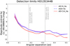 |
Fig. 5 Contrast curves for HD135344 B. The vertical lines indicate the outer radii of the cavities in small and large dust grains presented in Garufi et al. (2013) and Andrews et al. (2011), respectively. |
4.3 TW Hya
The TW Hya dataset does not show any point source either in the 1′′. 08 × 1′′.08 images (see Fig. 6) or in the 2′′.88 × 2′′.88 images, which are large enough to probe all the previously reported disk gaps. The final contrast curves are shown in Fig. 7. We also looked specifically at detection limits within the gaps observed by van Boekel et al. (2017) and focused in particular on the dark annulus at 20 AU (0′′. 39) from the central star, which has a counterpart approximately at the same position in 870 μm dust continuum observations (Andrews et al. 2016).
Since the circumstellar disk has a very small inclination, we considered the disk to be face-on and assumed the gaps to be circular. At 0′′.39, planets with contrast lower than 9.3 mag with respect to TW Hya would have been detected with the ASDI technique (cf. Fig. 7). This value was then combined with the stellar flux calculated as described in Sect. 4.1.4, to obtain the upper limit of the companion flux in the B_Ha filter. This yielded Ṁ < 1.0 × 10⁻¹¹ M⊙yr−1 (see Table 4) as the upper limit for the mass accretion rate based on our SPHERE/ZIMPOL dataset.
4.4 HD100546
The HD100546 dataset suffered from rather unstable and varying observing conditions, which resulted in a large dispersion in the recorded flux (see Fig. E.1). We hence selected only the last 33% of the observing sequence, which had relatively stable conditions, for our analysis (see Appendix E). The Hα data did notconfirm either of the two protoplanet candidates around HD100546 (see Fig. 6) and we show the resulting detection limits in Fig. 8.
In order to investigate the detection limits at the positions of the protoplanet candidates, we injected artificial planets with increasing contrast starting from ΔB_Ha = 8.0 mag until the signal was no longer detected with a CL of at least 99.99995%, and we repeated the process subtracting different numbers of PCs (from 10 to 30). At the position where Quanz et al. (2015) claimed the presence of a protoplanetary companion, we would have been able todetect objects with a contrast lower than 11.4 mag (using PC = 14 and the ADI reduction). Consequently, if existing, a 15 MJ companion (Quanz et al. 2015) located at the position of HD100546 b must be accreting at a rate < 6.4 × 10⁻¹² M⊙yr−1 in the framework of our analysis and assuming no dust is surrounding the object. We note that, in comparison to the accretion luminosity Lacc estimated by Rameau et al. (2017), our upper limit is one order of magnitude lower (cf. Table 4).
For the position of HD100546 c, we used the orbit given in Brittain et al. (2014) to infer the separation and PA of the candidate companion at the epoch of our observations, i.e., ρ ≃ 0′′.14 and PA ≃ 133°. At this position our data reach a contrast of 9.3 mag (using PC = 14 on the continuum-subtracted dataset), implying an upper limit for the companion flux in the Hα filter of 7.9 × 10⁻¹⁴ erg s−1 cm−2 and a mass accretion rate < 1.1 × 10⁻¹⁰ M⊙yr−1. This puts ~2 orders of magnitude stronger constraints on the accretion rate of HD100546 c than the limits obtained from the polarimetric Hα images presented in Mendigutía et al. (2017) for a 15 MJ planet. We note that owing to its orbit, HD100546 c is expected to have just disappeared or to disappear quickly behind the inner edge of the disk (Brittain et al. 2014). Therefore, extinction could play a major role in future attempts to detect this source.
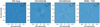 |
Fig. 6 Final PSF subtracted ADI images of TW Hya, HD100546, HD169142, and MWC 758. We applied a central mask with radius 32.4 mas and 18 PCs were removed. No companion candidates were detected. All images have a linear, but slightly different, color scale. |
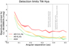 |
Fig. 7 Contrast curves for TW Hya. The vertical line indicates the gap at 0′′. 39 detected in both scattered light (Akiyama et al. 2015; van Boekel et al. 2017) and submillimeter continuum (Andrews et al. 2016). |
4.5 HD169142
We analyzed the data with ADI and ASDI reductions (see Fig. 6 for the ADI image). The latter was particularly interesting in this case because the stellar flux density in the continuum and Hα filter is very similar and the continuum subtraction almost annihilated the flux from the central PSF, indicating that the central star has limited to no Hα line emission (cf. Table 3 and see Grady et al. 2007). We calculated the detection limits as explained in Sect. 4.1.1 for both filters for a confidence level of 99.99995%, as shown in Fig. 9.
We investigated with particular interest the positions of the candidates mentioned in Sect. 2 and derived specific detection limits at their locations, independent from the azimuthally averaged contrast curve. At the position of the compact source found by Osorio et al. (2014; we call this potential source HD169142 c), our data are sensitive to objects 10.7 mag fainter than the central star (obtained by subtracting 16 PCs with ASDI reduction). At the position of HD169246 b (Reggiani et al. 2014; Biller et al. 2014) an object with a contrast as large as 9.9 mag could have been detected (PC = 19; ASDI). For the compact source from Osorio et al. (2014) we found Ṁ < 4.4 × 10⁻¹¹ M⊙yr−1. Similarly, for the object detected by Biller et al. (2014) and Reggiani et al. (2014)9 we found an upper limit for the mass accretion rate of Ṁ < 7.6 × 10⁻¹¹ M⊙yr−1.
4.6 MWC 758
Our analysis of the SPHERE/ZIMPOL images did not show an Hα counterpart to the MWC 758 companion candidate detected by Reggiani et al. (2018) as shown in Fig. 6. This is consistent with the recently published results from Huélamo et al. (2018). Nonetheless, we provide a detailed analysis and discussion of the same MWC 758 data to allow a comparison with the other datasets.
In Fig. 10 we show the detection limits obtained with ADI for the B_Ha and Cnt_Ha dataset, and the results of the ASDI approach. At separations larger than 0′′. 25, companions with a contrast smaller than 10 mag could have been detected. At the specific position of the candidate companion10 we can exclude objects with contrasts lower than 9.4 mag (obtained subtracting 15 PCs using ASDI).
To explain the presence of a gap in dust-continuum emission without a counterpart in scattered light, a steady replenishment of μm-sized particle is required, which implies that a companion in the inner disk should not exceed a mass of Mc = 5.5 MJ (Pinilla et al. 2015; Reggiani et al. 2018). In line with the analysis of Reggiani et al. (2018), we used the BT-Settl model to estimate the radius of the companion and we derived an upper limit for the mass accretion rate of Ṁ < 5.5 × 10⁻¹¹ M⊙yr−1 (see Table 4). Our analysis puts slightly stronger constraints on the mass accretion rate in comparison to that in Huélamo et al. (2018).
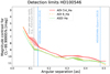 |
Fig. 8 Contrast curves for HD100546. The gray dashed vertical line shows the separation of the outer gap edge cavity presented in Avenhaus et al. (2014a), while the solid blue lines indicate the separations of the forming planet candidates around HD100546 (Quanz et al. 2013a; Brittain et al. 2014). |
5 Discussion
5.1 SPHERE/ZIMPOL as hunter for accreting planets
The SPHERE/ZIMPOL Hα filters allow for higher angular resolution compared to filters in the infrared regime and can, in principle, search for companions closer to the star. For comparison, a resolution element is 5.8 times smaller in the Hα filter than in the L′ filter, meaning that the inner working angle (IWA) is smaller by the same amount so that closer-in objects could be observed, if bright enough11. An instrument with similar capabilities is MagAO (Close et al. 2014b; Morzinski et al. 2016), but as the Magellan telescope has a primary mirror of 6.5 m diameter, it has a slightly larger IWA than SPHERE at the 8.2 m VLT/UT3 telescope. A direct comparison of the HD142527 B detection shows that ZIMPOL reaches a factor ~ 2.5 higher S/N in one-third of total integration time and field rotation of MagAO under similar seeing conditions, even if the companion is located ≳ 20 mas closer to the star. The VAMPIRES instrument combined with Subaru/SCExAO will soon be a third facility able to perform Hα imaging in SDI mode (Norris et al. 2012).
In terms of detection performance using different filters and reduction techniques, we re-emphasize that the N_Ha filter is more efficient in detecting Hα signals in the contrast limited regime. The smaller filter width reduces the contribution of the continuum flux, which often dominates the signal in the B_Ha filter, particularly for the central star. Hence, assuming the planetary companion emits only line radiation, the N_Ha filter reduces the contamination by the stellar signal in the remaining speckles. Moreover, the subtraction of the stellar continuum from Hα images reduces the speckles in both B_Ha and N_Ha filters. Hence, ASDI enhances the signal of potential faint companions, in particular at separations <0′′.3 (cf. Figs. 7, 9, 10), where companions 0.7 mag fainter appear accessible in comparison to using simple ADI. ASDI should always be applied during the analysis of SPHERE/ZIMPOL Hα data.
What remains to be quantified is how longer detector integration times (DITs) or the broad band filter could improve the detection limits in the background limited regime (i.e., > 0′′.3 where the contrast curves are typically flattening out) or for fainter natural guide stars. At these separations narrow band data can be detector read noise limited and the B_Ha filter might be more suitable because of its higher throughput. However, as we show in Fig. 11, it seems that at least for our HD142527 dataset this does not seem to be the case. Futurestudies conducted in both filters and on several objects are required to derive a more comprehensive understanding. Finding the sweetspot between longer integration times and the smearing of the PSF because of field rotation is also warranted. At least for the object considered in Fig. 11, at large separations (usually > 0′′.3, in the background limited region) it is even possible to ignore completely ADI and simply apply field stabilized observations.
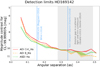 |
Fig. 9 Contrast curves for HD169142. The shaded region represents the annular gap observed in scattered light (Quanz et al. 2013b) and in millimeter continuum (Osorio et al. 2014). The blue vertical lines represent the separation of the companion candidates (Reggiani et al. 2014; Biller et al. 2014; Osorio et al. 2014). |
5.2 Constraining planet accretion
For our mass accretion rate estimates of HD142527 B we assumed that 100% of the Hα flux originates from accretion processes involving circumstellar material. We note, however, that the values may be overestimated if we consider that chromospheric activity of the M star (White & Basri 2003; Fang et al. 2009) can also contribute to the measured line flux. Furthermore, as mentioned in Sect. 4.1.5, we warn that the narrow width of the N_Ha filter might be too narrow to fully encompass all Hα line emission from fast-moving, accreting material, and therefore the results may be underestimated. Finally, given the presence of dusty material at the projected position of HD142527 B (Avenhaus et al. 2017), Hα flux might have been partially absorbed. It is beyond the scope of this paper to properly estimate a value for intrinsic extinction due to disk material and consider this value in the Ṁ estimation. Nevertheless, in Fig. 12 we show the fraction of Hα flux that is potentially lost because of extinction asa function of AV, converted into AHα as explained in Sect. 4.1.4. Only 2% of the Hα signal remains if the disk material causes an extinction of AV = 5 mag. This plot quantifies the impact of dust on the measured flux and the detectability of Hα emission from embedded objects.
For the other five objects studied in this work we were not able to detect any clear accretion signature located in the disks. Therefore, our data were not able to support the scenario in which protoplanets are forming in those disks. We put upper limits on the accretion luminosity and mass accretion rate. Two notes have to be made: (1) the fundamental quantities directly derived from the data are FHα and LHα; they should be used for future comparisons with other datasets or objects; (2) the presented upper limits on Ṁ are only valid for an object with the mass and radius given in Table 4, while the Lacc upper limits refer to objects of any mass. In particular, assuming lower mass objects implies larger Ṁ, as shown in Fig. 13: on the y-axis the mass accretion rate upper limits decrease as a function of the companion mass, for which the corresponding radius was calculated using the evolutionary models reported in Table 4 and assuming the age listed in Table 2. The plot highlights that the assumed mass of the companion may change the final Ṁacc by more than one order of magnitude. Moreover, we overplot in violet the mass accretion rates of the three objects presented in Zhou et al. (2014, see also Sect. 5.3) as well as LkCa15 b and PDS70 b (Sallum et al. 2015; Wagner et al. 2018), and in gray the range of mass accretion rates for HD142527 B.
We stress that, similar to HD142527 B, we always assumed that the flux limit is completely due to Hα line emission without any contribution from continuum or chromospheric activity. Furthermore, for our analysis we always neglected intrinsic extinction effects from disk material, which likely weaken the signal. In particular, at locations where no gap in small dust grains has been identified the extinction AHα can be significant (see Fig. 12). Models and precise measurements of the dust content in the individual disks would be required to properly include local extinction into our analysis. Finally, investigating the Hα luminosity upper limits for the specific positions as a function of the separation from the central star, it can be noticed that the constraints are stronger at larger separations. The only exception is HD100546, for which higher upper limits were achieved. The combinationof suboptimal weather conditions, under which the dataset was taken, and the small field rotation of the subsample analyzed in this work made those limits worse. A more stable dataset with larger field rotation should provide more constraining limits.
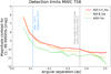 |
Fig. 10 Contrast curves for MWC 758. The gray dashed line shows the outer edge of the dust cavity observed by Andrews et al. (2011). The blue solid line indicates the separation at which Reggiani et al. (2018) found a candidate companion. |
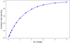 |
Fig. 11 Apparent flux detection limits as a function of the angular separation from HD142527 for both B_Ha and N_Ha filters. |
5.3 Comparison with other objects
The accretion rate of HD142527 B is in good agreement with the mass accretion rates found in Rigliaco et al. (2012) for low-mass T Tauri stars in the σ Ori star-formingregion (5 × 10⁻¹¹ M⊙yr−1 < ṀCTTS < 10−9 M⊙yr−1). A slightly broader mass accretion rate range was found by Alcalá et al. (2014), with 2 × 10⁻¹² M⊙yr−1 < ṀCTTS < 4 × 10⁻⁸ M⊙yr−1 in the Lupus star-formingregion. Zhou et al. (2014) reported three very low-mass objects (GSC 06214-00210 b, GQ Lup b and DH Tau b), which exhibit Hα emission from accretion. Those objects have separations of 100–350 AU from their parent stars and Ṁ ~ 10−9−10−11 M⊙yr−1 (see violet stars in Fig. 13). The accretion rates measured in the paper are of the same order as thelimits we found in our work. At projected distances similar to those of the three objects mentioned above, ZIMPOL would have been able to observe and detect Hα emitting companions. However, closer to the star in the contrast limited regime, our data would not have detected accretion processes occurring with Ṁ ≲ 10−11 M⊙yr−1.
The mass accretion rate of PDS70 b was estimated by Wagner et al. (2018) without considering any extinction effects and it is slightly lower than the limits we achieve for our sample (see violet square in Fig. 13 and black star in Fig. 14). The flux was calculated from the contrast in Wagner et al. (2018) assuming RPDS70 b = 11.7 mag and estimating the MagAO Hα filter widths assuming a flat SED12. In order to properly compare our limits and their Hα detection, the same confidence levels should be considered. We therefore estimated the contrast limit for a CL corresponding to a 4σ detection for HD142527 at the separation of PDS70 b, which was 0.3 mag lower than the limits corresponding to a CL of 99.99995%. Hence, to bring all the contrast curves from Fig. 14 to a 4σ confidence level at ~0′′.19, a multiplication by a factor 0.76 is required. We note, however, that this scaling is just an approximation to provide a more direct comparison between the two studies.
We also compared the Hα line luminosity upper limits obtained from our ZIMPOL Hα sample with that estimated by Sallum et al. (2015) for LkCa15 b (LHα ~ 6 × 10⁻⁵ L⊙). Our specific limits for the candidates around HD169142, HD100546, and MWC 758 are slightly lower, but, except for HD100546 b and the compact source in HD169142 found by Osorio et al. (2014), of the same order of magnitude. LkCa15 itself was observed with SPHERE/ZIMPOL during the science verification phase in ESO period P96. We downloaded and analyzed the data, which were, however, poor in quality and also in terms of integration time and field rotation. Only ~ 1 h of data is available with a field rotation of ~16°, a coherence time of 2.6 ± 0.8 ms, and a mean seeing of 1′′.64 ± 0′′.37. As we show in Fig. 14, with deeper observations including more field rotation, ZIMPOL can potentially detect the signal produced by LkCa15 b (Sallum et al. 2015) with a CL of 99.99995%. However, the higher airmass at the Paranal Observatoryand the fact that LkCa15 is a fainter guide star may complicate the redetection of the companion candidate, and therefore exceptional atmospheric conditions are required.
In addition to Hα also other spectral features like Paβ and Brγ lines may indicate ongoing accretion processes onto young objects. As an example, Daemgen et al. (2017) used the absence of those lines in the spectrum of the low-mass companion HD106906 b to infer its mass accretion rate upper limits (Ṁ < 4.8 × 10⁻¹⁰ MJ yr−1). Their constraint is stronger than the ones we were able to put with our ZIMPOL Hα data. Several other studies also detected hydrogen emission lines like Paβ from low-mass companions (e.g., Seifahrt et al. 2007; Bowler et al. 2011; Bonnefoy et al. 2014), but unfortunately they did not calculate mass accretion rates.
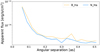 |
Fig. 12 Fraction of Hα flux absorbed as a function of the disk extinction AV assuming the extinction law of Mathis (1990) as explained in Sect. 4.1.4. |
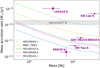 |
Fig. 13 Mass accretion rate upper limits as a function of the planetary mass for all the candidate forming planets investigated in this work. The violet stars represent the values reported in Zhou et al. (2014), while the violet squares indicate PDS70 b (Wagner et al. 2018) and LkCa15 b (Sallum et al. 2015). The gray shaded area represents the mass accretion rate of HD142527 B and is shown for mass accretion rate comparisonpurposes only. Indeed, the mass of the object is much larger than what is reported on the x-axis of the plot. |
5.4 Comparison with existing models
Two models for planetary accretion are currently used to explain the accreting phase of planet formation: magnetospheric accretion (Zhu 2015) and boundary layer accretion (Owen & Menou 2016). During magnetospheric accretion, the magnetic field truncates the CPD and hot ionized hydrogen in the closest regions of the disk falls onto the planet following the magnetic field lines. Recombination on the planet surface then produces Hα flux. For protoplanets, these models predict Hα luminosities at least three orders of magnitudes lower than in CTTS, according to Eq. (22) in Zhu (2015),
 (5)
(5)
This is mainly owing to a one order of magnitude smaller infall velocity vs and a one order of magnitude smaller truncation radius RT (squared in the LHα equation) due to weaker magnetic fields than in stars. We combined the magnetospheric accretion models (Zhu 2015) with existing detections in the infrared and evolutionary models. As an example, we present the case of HD100546 b. According to models (Zhu 2015), the observed L′ brightness could be emitted by a CPD with inner radius of 1–4 RJ and MpṀ of  . The mass accretion constraints obtained from Hα ZIMPOL data would therefore imply that Mp ≳ 31 MJ. This result is in conflict with that obtained by Quanz et al. (2015) and the AMES-Cond evolutionary models, since the object L′ brightness excludes masses larger than ~15 MJ. This is the mass expected in the case in which the L′ flux is only from photospheric emission. Moreover, a 30 MJ object would have significantly shaped the disk morphology and would have been clearly visible in other bands, such as the Ks -band, where Quanz et al. (2015) could only put upper limits to the companion brightness.
Szulágyi & Mordasini (2017) found that only a minimal fraction of the hydrogen in CPDs might be thermally ionized if the planet is massive and hot enough. Consequently, the disk does not get truncated and ionized material does not get accreted through magnetospheric accretion along the field lines. Then, disk material falls directly onto the planet (boundary layer accretion). The same authors showed that material falling from the circumstellar disk onto the CPD and the protoplanet shocks, and eventually produces Hα line emission both from the CPD and the planet. The contribution to the Hα flux is larger from the CPD than from the planet (Szulágyi & Mordasini 2017). These authors also showed that the majority of the accreted gas, however, remains neutral, especially for planets <10 MJ. Hence, the Hα flux can only estimate the ionized gas accretion rate and not the total accreted material. According to their simulations, a 10 MJ planet would be accreting at a rate of 5.7 × 10⁻⁸ MJyr−1, producing LHα ~ 7 × 10⁻⁶ L⊙. This value is on the same order of the limits our data allow us to put on the Hα luminosity from known forming protoplanet candidates. Since considering lower planetary masses enhances the mass accretion rate (see Eq. (4)) and higher masses should be visible in other infrared bands, we conclude that either extinction from disk material plays a major role in the nondetection of the existing candidates, or they are false positives resulting from image post-processing.
The comparison of LHα limits from Table 4 with Fig. 7 from Mordasini et al. (2017) indicates that, assuming completely cold accretion, the observed objects may be low-mass (0.1−1MJ) medium accreters (Ṁ ~ 10−10–10−9M⊙ yr−1) or higher mass objects (1−15MJ) showing very little accretion (Ṁ < 10−10.5M⊙ yr−1). Mordasini et al. (2017) also suggested another possible reason for some of the nondetections in Hα. If some of the planets, such as HD100546 b, have not yet completely detached from the disk, they would be cooler and would not be accreting at high accretion rates. In a later phase, they will possibly be able to open a gap and accrete a large amount of material.
Another aspect that we did not consider is the effect of the circumplanetary disk inclination on the flux that is emitted. Zhu (2015) considered the disk inclination including a factor 1∕cos(i), where i is the CPD inclination. Detailed accretion models should investigate the consequences of a tilted protoplanetary disk on LHα.
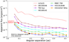 |
Fig. 14 Detection limits in apparent flux obtained for a 99.99995% CL in this work, together with limits achieved with the available ZIMPOL dataset for LkCa15 b (red dashed line) and the result presented in Sallum et al. (2015) and Wagner et al. (2018). A deeper dataset is required to redetect LkCa15 b with ZIMPOL, but this detection is feasible. |
6 Conclusions
Imaging in Hα is one of the promising techniques to detect forming planets at very small separations. In this context, the SPHERE/ZIMPOL instrument will play a major role in investigating local accretion signatures in circumstellar disks. An important next step is to redetect the previous discoveries of MagAO of Hα emission from LkCa15 b and PDS 70 b and to study potential accretion variability. None of the possible protoplanet candidates discovered in the infrared (HD169142 b, MWC758 b, and HD100546 b and c) could be confirmed in this study searching for accretion signatures, implying several possible scenarios. Their mass accretion rates could be lower than our limits and therefore they are currently not detectable. Other explanations are that protoplanetary accretion shows variability and some of the objects are currently going through a period of quiescence, or that extinction effects from disk material absorb a considerable fraction of the light. The study of NIR line diagnostics might reduce the effects of absorption and allow the detection of accretion processes. Furthermore, it is possible that the observed candidates are disk features that have been enhanced by image post-processing (Follette et al. 2017; Ligi et al. 2018), or our understanding of accretion processes during the formation of giant planets is not correct and, as an example, the use of the CTTS scaling relation is not correct. In order to investigate this, precise simulations of protoplanetary accretion, as well as of disk intrinsic effects (via full radiative transfer), have to be developed and combined with multiwavelength observations spanning from the optical to the (sub)millimeter.
The estimation of upper limits are of particular importance for the study of accretion variability of protoplanets in the future. Continuing surveys for accreting planets could possibly detect Hα signatures and combine these with detection limits provided by this work to investigate variability in the accretion processes. Finally, we emphasize that although a lot of effort was put into the calculation of mass accretion rate upper limits, those values are model and parameter dependent. The Hα flux upper limits are, however, the fundamental quantities that were measured from the data and can be directly compared with future observations.
Acknowledgements
SPHERE is an instrument designed and built by a consortium consisting of IPAG (Grenoble, France), MPIA (Heidelberg, Germany), LAM (Marseille, France), LESIA (Paris, France), Laboratoire Lagrange (Nice, France), INAF – Osservatorio di Padova (Italy), Observatoire de Genéve (Switzerland), ETH Zurich (Switerland), NOVA (Netherlands), ONERA (France), and ASTRON (Netherlands), in collaboration with ESO. SPHERE also received funding from the European Commission Sixth and Seventh Framework Programmes as part of the Optical Infrared Coordination Network for Astronomy (OPTICON) under grant number RII3-Ct-2004-001566 for FP6 (2004–2008), grant number 226604 for FP7 (2009–2012), and grant number 312430 for FP7 (2013–2016). This work has been carried out within the frame of the National Center for Competence in Research PlanetS supported by the Swiss National Science Foundation. S.P.Q. and H.M.S. acknowledge the financial support of the SNSF. G.C. and S.P.Q. thank the Swiss National Science Foundation for financial support under grant number 200021_169131. F.M. and G.v.d.P. acknowledge fundings from ANR of France under contract number ANR-16-CE31-0013. This research has made use of the SIMBAD database, operated at CDS, Strasbourg, France. This work has made use of data from the European Space Agency (ESA) mission Gaia (https://www.cosmos.esa.int/gaia), processed by the Gaia Data Processing and Analysis Consortium (DPAC, https://www.cosmos.esa.int/web/gaia/dpac/consortium). Funding for the DPAC has been provided by national institutions, in particular the institutions participating in the Gaia Multilateral Agreement. The authors thank Arianna Musso-Barcucci for the preliminary analysis on HD142527.
Appendix A Influence of the beamsplitter on flux measurements
We investigated the effects of the throughput uncertainties of the two ZIMPOL arms resulting from instrument polarization effects. It is currently not known how the overall throughput to the individual ZIMPOL arms depends on the telescope and instrument configurations. However, it is easy to estimate the overall effect because the Nasmyth mirror of the VLT introduces an instrument polarization of about 4%. This is reduced by the first mirror in SPHERE to about 0 to 3%, while the following mirrors in the instrument add further positive or negative polarization contributions of about 2%, while polarization cross talks (linear → circular polarization) reduce the linear polarization. Thus, it is safe to adopt a maximum error of 5% for the relative difference (e.g., T(Hα) = (1 ± 0.05)T(cont)) in throughput between the two channels. We therefore tested the impact of an enhancement/decrease by at most 5% in the continuum flux, analyzing the consequences on the detection of HD142527B and on the contrast performances of our pipeline. The signal flux is measured in an aperture of radius 8.3 mas, and the FPF was calculated as explained in Sect. 4.1.1. The results averaged over a range of PCs (PC = 10, 15, 20, 25, 30) on the ASDI-processed B_Ha dataset are shown in Table A.1; a central mask of 21.6 mas was applied. As one may expect, the signal flux shows a strong variation of 20– 50% in the ASDI images, which is mainly due to the stronger/weaker subtraction of the continuum. The relative difference in this case is increased from the initial 5% by the ASDI processing, but it should be noted that together with the signal, the noise level also gets increased/decreased, causing the FPF to be less subject to variations. Indeed, regarding the FPF values, we argue that depending on the arm 1 to arm 2 transmission the confidence of the detection is lower by a factor of ~ 10 in both extreme cases, which corresponds approximately to a maximum variation of ~ 0.1 mag in Δmag. Therefore, we do not expect this effect to have a large impact on the detection limits estimated in this work. Nevertheless, it is important to keep in mind that the calculation of the mass accretion rate of HD142527 B does not considerthis effect and a more accurate description of the instrument behavior is required to correct for it.
Resulting signal flux and FPF for different beamsplitter behaviors.
Appendix B FPF analysis of the HD142527 B dataset
In order to identify the best strategy for future SPHERE/ZIMPOL observations, we compared the FPF calculated after
the subtraction of different numbers of PCs using different techniques and datasets. For the ADI technique we considered three datasets: B_Ha, N_Ha, and Cnt_Ha, of which the last set contained all the images taken with the continuum filter. For SDI and ASDI, we considered the subtraction of the Cnt_Ha images from the respective Hα filter images. All the images had a size of 1′′.08 × 1′′.08. For each case, we applied an inner mask of varying size (10.8 mas, 21.6 mas, 32.4 mas) and chose the smallest FPF value as representative value for the detection. The FPF calculation (see Sect. 4.1.1) followed the prescription suggested in Mawet et al. (2014). Because of the strong negative wings of the companion in the PSF subtracted images, we decided not to consider thetwo background apertures closest to the signal as they are not representative of the background and speckle noise.
In the four panels of Fig. B.1 we analyzed the FPFs of HD142527 B, obtained using different combinations of techniques and datasets. In the top panels we compare the detection from different filters using the same technique: ADI on the left and ASDI on the right. For the ADI analysis, the B_Ha and Cnt_Ha datasets show similar values with a stronger detection in B_Ha forfewer subtracted components, while the FPF values obtained with the N_Ha filter are, for a wide range of PCs (from 11 to 32), ~5 orders of magnitude lower. The detections with the ASDI technique show a similar trend; there is a stronger detection in N_Ha, particularly between 10 and 27 PCs. The normal SDI technique, which is not presented in the image, was not efficient enough to properly subtract the stellar PSF and did not reveal the companion. This is probably for two reasons: (1) the central star is actively accreting material and emitting strong Hα flux, which cannot be subtracted accurately with the Cnt_Ha images, impeding the detection of the companion, and (2) PSF shapes are slightly different for different filters due to nonmatching bandpasses.
In the lower panels, we consider the results from the B_Ha (left) and N_Ha (right) datasets for ADI and ASDI. In both cases ASDI seems to be more efficient in detecting signals. A larger gain is obtained for the B_Ha filter, while FPFs obtained with the N_Ha filter have more similar values, probably due to the minor impact of the continuum subtraction on images taken with the narrow filterwith respect to the broad filter. We conclude that the best observing strategy to look for accreting companions in the contrast limited regime with SPHERE/ZIMPOL is to take images in the N_Ha filter and Cnt_Ha filter simultaneously and to perform ASDI. It is of particular interest that in the case of HD142527, ASDI also performs better than ADI. Indeed, we could expect that the presence of a clear signal in the continuum would have strongly compromised the detection with ASDI. On the contrary, the detection is even stronger, implying that the subtraction of the stellar pattern is much more important than the self-subtraction of the companion, boosting its S/N. We note, however, that observing fainter objects might cause the data to be readout noise limited. In this case, the B_Ha filter might be preferred to the N_Ha filter. This hypothesis, however, should be confirmed with a fainter source than the bright M-dwarf HD142527B.
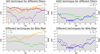 |
Fig. B.1 Performance comparison for Hα imaging with SPHERE/ZIMPOL using different filters (narrow and broad Hα) and reduction techniques (ADI and ASDI) based on the HD142527 dataset. In all panels the FPF obtained for HD142527 B is shown, as a function of the number of subtracted PCs used in PynPoint. On the right side of each panel we give the scale of the S/N to improve understanding of the plot and to compare different instrumental setups. We note again that this does not correspond to the classical σ notation. The gray regions indicates a confidence level for the detection of HD142527 B of at least 99.99995%, i.e., >5σ in case of Gaussian noise. Because of the applied corrections for small sample statistics, the border of the gray area does not correspond to an S/N of 5. |
Appendix C Impact of field rotation and total integration time
In addition to the best instrumental setup for the detection of accreting objects in Hα imaging, we also investigated the effect of two observational parameters on the achieved upper limits: the field rotation and integration time on target. Two subsets were created from the HD142527 B_Ha data. The first was composed of every second frame of thedataset, while the second only included the first half of the dataset frames. In this way, the field rotation of the first subset is twice that of the second subset, while the integration time is the same for the two subsets. Figure C.1 shows the resulting contrast curves, calculated in the same way as described in Sect. 4.1.1. The dashed blue line represents the subset composed of the first half of the dataset, which allows us to reach ~ 9.4 mag of contrast at 0′′.2. The green solid line shows the contrast limits estimated from the subset composed of every second frame. It is clear that at all separations, this subset allows us to detect fainter objects than the other subset and at 0′′. 2 the difference reaches 1.1 mag. Finally, the entire dataset allows us to go, at the same distance, another 0.3 mag deeper. At least for this dataset, the field rotation seems to play a very important role, allowing a better modeling and subtraction of the stellar PSF.
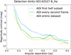 |
Fig. C.1 Contrast curves calculated for the “first half” (blue dashed line) and the “very second frame” subsets (green solid line), and for the entire B_Ha dataset of HD142527 (orange dotted line). |
Appendix D Is a companion candidate orbiting HD135344B?
We visually inspected the final PSF-subtracted ADI images of HD135344 B, which showed a potential signal north of thestar. The feature is persistent in the N_Ha and Cnt_Ha datasets for different mask radii (e.g., 0′′. 02, 0′′. 03, 0′′. 04, 0′′. 05, and 0′′. 06) and over a wide range of PCs (6-21). In particular, when using larger mask radii, the close-in speckles are removed and the signal appears to be stronger. We then investigated smaller images (101 × 101 pixels) with the same technique and confirmed the signal for different mask radii and PCs. Next, we examined the ASDI images and found that the signal is present once again in different reductions, but appears fainter. If the signal is from a physical source, this is expected from an accreting object emitting Hα line radiation. This signal is shown in Fig. D.1 in the N_Ha and in the Cnt_Ha filter for the parameter setups that yield the lowest FPFs, which are 5.9 × 10⁻⁵ for N_Ha and 0.0015 for Cnt_Ha.
A careful look at the bright signal in the Cnt_Ha images raises doubts on the nature of its source as it is very compact and does not have a PSF-like shape. Furthermore, the signal has high FPFs, with a minimal value of ~ 0.0015, which is notstatistically significant enough to claim a detection.
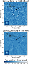 |
Fig. D.1 Lowest FPF images of HD135344 B (top panel: N_Ha filter; bottom panel: Cnt_Ha filter). The radius r of the inner mask and the number of subtracted PCs are given in each panel. The location of the tentative companion candidate is indicated by the arrow (see Sect. 4.1.2). |
The signal in the N_Ha frames has a morphology resembling that of a faint physical source. Varying the number of PCs seems to influence the apparent shape and location of the signal, as expected from faint close-in objects with low S/N when subtracting the stellar PSF. Even though for 9 PCs the FPF reaches a minimal value of ~ 5.9 × 10⁻⁵, the FPFs for 7–17
PCs are in the range 10−3−10−2, which does not give us sufficient confidence to claim a detection.
As a final check, we used the Hessian matrix approach as described in Sect. 4.1.2 to perform a signal characterization. We ran the algorithm for PCs between 7 and 17 (where the final images showed a clear signal) with a central mask of radius 57.6 mas and a ROI of 8 × 8 pixels. The other parameters were kept identical to the analysis performed on HD142527 B. The signal appears to be located at a separation of  mas with a PA of
  . The contrast was measured to be 8.1 ± 0.4 mag. As visible in the error bars, the positions found are spread over a range of ~ 9 mas, which corresponds to ~2.5 pixels. Normally, a physical point source should be less affected by systematics introduced by the PSF subtraction process. However, a low S/N object at a separation of 71.1 mas is more difficult to measure properly and a larger spread in the recovered positions could be the result. A similar note can be made for the contrast values, which span over a range of ~ 0.8 mag. We conclude that to settle this issue and fully understand the origin of the signal in the Hα filter, a dataset with higher S/N would be required.
Appendix E Frame selection for the HD100546 dataset
As briefly described in Sect. 4.4, the large HD100546 dataset (1104 frames, cf. Table 1) was taken in unstable conditions, which made a frame selection necessary. To determine a frame selection metric, we plotted the mean count value per image (image dimensions 1′′.08 × 1′′.08 pixels, see Fig. E.1). It turned out that three phases could be identified within the observing run: a short initial phase of stability with some outliers (120 frames), a long period of 619 frames where the mean count values spanned a range between ~ 0 and ~55 counts per pixels, and, finally, a large amount of stable frames at the end of the observations (mean pixel value ~ 55 in B_Ha). We decided only to keep the images of the last stable period, composed of the frames 739–1104 to perform our analysis. This subsample has a total on-target integration time of 61 min and its field rotation is ~ 20.7°.
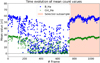 |
Fig. E.1 B_Ha (blue circles) and Cnt_Ha (green crosses) mean count rates as a function of the image number in the observing sequence. The shaded region at the end represents the subset of frames that was chosen for the analysis. |
References
- Akiyama, E., Muto, T., Kusakabe, N., et al. 2015, ApJ, 802, L17 [NASA ADS] [CrossRef] [Google Scholar]
- Alcalá, J. M., Natta, A., Manara, C. F., et al. 2014, A&A, 561, A2 [NASA ADS] [CrossRef] [EDP Sciences] [Google Scholar]
- Allard, F., Hauschildt, P. H., Alexander, D. R., Tamanai, A., & Schweitzer, A. 2001, ApJ, 556, 357 [NASA ADS] [CrossRef] [Google Scholar]
- Allard, F., Homeier, D., & Freytag, B. 2012, Phil. Trans. R. Soc. London, Ser. A, 370, 2765 [Google Scholar]
- Amara, A., & Quanz, S. P. 2012, MNRAS, 427, 948 [NASA ADS] [CrossRef] [Google Scholar]
- Amara, A., Quanz, S. P., & Akeret, J. 2015, Astron. Comput., 10, 107 [NASA ADS] [CrossRef] [Google Scholar]
- Andrews, S. M., Wilner, D. J., Espaillat, C., et al. 2011, ApJ, 732, 42 [NASA ADS] [CrossRef] [Google Scholar]
- Andrews, S. M., Wilner, D. J., Zhu, Z., et al. 2016, ApJ, 820, L40 [NASA ADS] [CrossRef] [Google Scholar]
- Augereau, J. C., Lagrange, A. M., Mouillet, D., & Ménard, F. 2001, A&A, 365, 78 [NASA ADS] [CrossRef] [EDP Sciences] [Google Scholar]
- Avenhaus, H., Quanz, S. P., Meyer, M. R., et al. 2014a, ApJ, 790, 56 [NASA ADS] [CrossRef] [Google Scholar]
- Avenhaus, H., Quanz, S. P., Schmid, H. M., et al. 2014b, ApJ, 781, 87 [NASA ADS] [CrossRef] [Google Scholar]
- Avenhaus, H., Quanz, S. P., Schmid, H. M., et al. 2017, AJ, 154, 33 [NASA ADS] [CrossRef] [Google Scholar]
- Baraffe, I., Chabrier, G., Barman, T. S., Allard, F., & Hauschildt, P. H. 2003, A&A, 402, 701 [NASA ADS] [CrossRef] [EDP Sciences] [Google Scholar]
- Benisty, M., Juhasz, A., Boccaletti, A., et al. 2015, A&A, 578, L6 [NASA ADS] [CrossRef] [EDP Sciences] [Google Scholar]
- Bertrang, G. H.-M., Avenhaus, H., Casassus, S., et al. 2018, MNRAS, 474, 5105 [NASA ADS] [CrossRef] [Google Scholar]
- Beuzit, J.-L., Feldt, M., Dohlen, K., et al. 2008, in Ground-based and Airborne Instrumentation for Astronomy II, Proc. SPIE, 7014,701418 [CrossRef] [Google Scholar]
- Biller, B., Lacour, S., Juhász, A., et al. 2012, ApJ, 753, L38 [NASA ADS] [CrossRef] [Google Scholar]
- Biller, B. A., Males, J., Rodigas, T., et al. 2014, ApJ, 792, L22 [NASA ADS] [CrossRef] [Google Scholar]
- Boehler, Y., Ricci, L., Weaver, E., et al. 2018, ApJ, 853, 162 [Google Scholar]
- Bonnefoy, M., Chauvin, G., Lagrange, A.-M., et al. 2014, A&A, 562, A127 [NASA ADS] [CrossRef] [EDP Sciences] [Google Scholar]
- Boss, A. P. 1997, Science, 276, 1836 [NASA ADS] [CrossRef] [Google Scholar]
- Bowler, B. P., Liu, M. C., Kraus, A. L., Mann, A. W., & Ireland, M. J. 2011, ApJ, 743, 148 [NASA ADS] [CrossRef] [Google Scholar]
- Brittain, S. D., Najita, J. R., Carr, J. S., et al. 2013, ApJ, 767, 159 [NASA ADS] [CrossRef] [Google Scholar]
- Brittain, S. D., Carr, J. S., Najita, J. R., Quanz, S. P., & Meyer, M. R. 2014, ApJ, 791, 136 [NASA ADS] [CrossRef] [Google Scholar]
- Calvet, N., & Gullbring, E. 1998, ApJ, 509, 802 [NASA ADS] [CrossRef] [Google Scholar]
- Canovas, H., Ménard, F., Hales, A., et al. 2013, A&A, 556, A123 [NASA ADS] [CrossRef] [EDP Sciences] [Google Scholar]
- Christiaens, V., Casassus, S., Absil, O., et al. 2018, A&A, 617, A37 [NASA ADS] [CrossRef] [EDP Sciences] [Google Scholar]
- Claudi, R., Maire, A.-L., Mesa, D., et al. 2019, A&A, 622, A96 [NASA ADS] [CrossRef] [EDP Sciences] [Google Scholar]
- Cleeves, L. I., Bergin, E. A., & Harries, T. J. 2015, ApJ, 807, 2 [NASA ADS] [CrossRef] [Google Scholar]
- Close, L. M., Follette, K. B., Males, J. R., et al. 2014a, ApJ, 781, L30 [NASA ADS] [CrossRef] [Google Scholar]
- Close, L. M., Males, J. R., Follette, K. B., et al. 2014b, in Adaptive Optics Systems IV, Proc. SPIE, 9148, 91481M [CrossRef] [Google Scholar]
- Currie, T., Cloutier, R., Brittain, S., et al. 2015, ApJ, 814, L27 [NASA ADS] [CrossRef] [Google Scholar]
- Daemgen, S., Todorov, K., Quanz, S. P., et al. 2017, A&A, 608, A71 [NASA ADS] [CrossRef] [EDP Sciences] [Google Scholar]
- Debes, J. H., Jang-Condell, H., Weinberger, A. J., Roberge, A., & Schneider, G. 2013, ApJ, 771, 45 [NASA ADS] [CrossRef] [Google Scholar]
- Eisner, J. A. 2015, ApJ, 803, L4 [NASA ADS] [CrossRef] [Google Scholar]
- Fairlamb, J. R., Oudmaijer, R. D., Mendigutía, I., Ilee, J. D., & van den Ancker, M. E. 2015, MNRAS, 453, 976 [NASA ADS] [CrossRef] [Google Scholar]
- Fang, M., van Boekel, R., Wang, W., et al. 2009, A&A, 504, 461 [NASA ADS] [CrossRef] [EDP Sciences] [Google Scholar]
- Fedele, D., Carney, M., Hogerheijde, M. R., et al. 2017, A&A, 600, A72 [NASA ADS] [CrossRef] [EDP Sciences] [Google Scholar]
- Follette, K. B., Rameau, J., Dong, R., et al. 2017, AJ, 153, 264 [NASA ADS] [CrossRef] [Google Scholar]
- Fukagawa, M., Tamura, M., Itoh, Y., et al. 2006, ApJ, 636, L153 [NASA ADS] [CrossRef] [Google Scholar]
- Fukagawa, M., Tsukagoshi, T., Momose, M., et al. 2013, PASJ, 65, L14 [NASA ADS] [CrossRef] [Google Scholar]
- Fusco, T., Sauvage, J.-F., Mouillet, D., et al. 2016, in Adaptive Optics Systems V, Proc. SPIE, 9909, 99090U [CrossRef] [Google Scholar]
- Gaia Collaboration (Brown, A. G. A., et al.) 2018, A&A, 616, A1 [NASA ADS] [CrossRef] [EDP Sciences] [Google Scholar]
- Garufi, A., Quanz, S. P., Avenhaus, H., et al. 2013, A&A, 560, A105 [NASA ADS] [CrossRef] [EDP Sciences] [Google Scholar]
- Grady, C. A., Schneider, G., Hamaguchi, K., et al. 2007, ApJ, 665, 1391 [NASA ADS] [CrossRef] [Google Scholar]
- Grady, C. A., Muto, T., Hashimoto, J., et al. 2013, ApJ, 762, 48 [NASA ADS] [CrossRef] [Google Scholar]
- Gullbring, E., Hartmann, L., Briceño, C., & Calvet, N. 1998, ApJ, 492, 323 [NASA ADS] [CrossRef] [Google Scholar]
- Hartmann, L., Hewett, R., & Calvet, N. 1994, ApJ, 426, 669 [NASA ADS] [CrossRef] [Google Scholar]
- Henden, A. A., Templeton, M., Terrell, D., et al. 2016, VizieR Online Data Catalog: II/336 [Google Scholar]
- Huang, J., Andrews, S. M., Cleeves, L. I., et al. 2018, ApJ, 852, 122 [NASA ADS] [CrossRef] [Google Scholar]
- Huélamo, N., Chauvin, G., Schmid, H. M., et al. 2018, A&A, 613, L5 [NASA ADS] [CrossRef] [EDP Sciences] [Google Scholar]
- Keppler, M., Benisty, M., Müller, A., et al. 2018, A&A, 617, A44 [NASA ADS] [CrossRef] [EDP Sciences] [Google Scholar]
- Kraus, A. L., & Ireland, M. J. 2012, ApJ, 745, 5 [NASA ADS] [CrossRef] [Google Scholar]
- Lacour, S., Biller, B., Cheetham, A., et al. 2016, A&A, 590, A90 [NASA ADS] [CrossRef] [EDP Sciences] [Google Scholar]
- Lambrechts, M., & Johansen, A. 2012, A&A, 544, A32 [Google Scholar]
- Ligi, R., Vigan, A., Gratton, R., et al. 2018, MNRAS, 473, 1774 [NASA ADS] [CrossRef] [Google Scholar]
- Lyo, A.-R., Ohashi, N., Qi, C., Wilner, D. J., & Su, Y.-N. 2011, AJ, 142, 151 [NASA ADS] [CrossRef] [Google Scholar]
- Macintosh, B., Graham, J., Palmer, D., et al. 2006, Proc. SPIE, 6272, 62720L [CrossRef] [Google Scholar]
- Maire, A.-L., Langlois, M., Dohlen, K., et al. 2016, in Ground-based and Airborne Instrumentation for Astronomy VI, Proc. SPIE, 9908, 990834 [CrossRef] [Google Scholar]
- Maire, A.-L., Stolker, T., Messina, S., et al. 2017, A&A, 601, A134 [NASA ADS] [CrossRef] [EDP Sciences] [Google Scholar]
- Marleau, G.-D., Klahr, H., Kuiper, R., & Mordasini, C. 2017, ApJ, 836, 221 [Google Scholar]
- Marois, C., Lafrenière, D., Doyon, R., Macintosh, B., & Nadeau, D. 2006, ApJ, 641, 556 [Google Scholar]
- Marois, C., Lafrenière, D., Macintosh, B., & Doyon, R. 2008, ApJ, 673, 647 [NASA ADS] [CrossRef] [Google Scholar]
- Mathis, J. S. 1990, ARA&A, 28, 37 [NASA ADS] [CrossRef] [Google Scholar]
- Mawet, D., Milli, J., Wahhaj, Z., et al. 2014, ApJ, 792, 97 [NASA ADS] [CrossRef] [Google Scholar]
- Meeus, G., Montesinos, B., Mendigutía, I., et al. 2012, A&A, 544, A78 [NASA ADS] [CrossRef] [EDP Sciences] [Google Scholar]
- Mendigutía, I., Oudmaijer, R. D., Garufi, A., et al. 2017, A&A, 608, A104 [NASA ADS] [CrossRef] [EDP Sciences] [Google Scholar]
- Mordasini, C., Marleau, G.-D., & Mollière, P. 2017, A&A, 608, A72 [NASA ADS] [CrossRef] [EDP Sciences] [Google Scholar]
- Morzinski, K. M., Close, L. M., Males, J. R., et al. 2016, in Adaptive Optics Systems V, Proc. SPIE, 9909, 990901 [CrossRef] [Google Scholar]
- Müller, A., van den Ancker, M. E., Launhardt, R., et al. 2011, A&A, 530, A85 [NASA ADS] [CrossRef] [EDP Sciences] [Google Scholar]
- Muto, T., Grady, C. A., Hashimoto, J., et al. 2012, ApJ, 748, L22 [NASA ADS] [CrossRef] [Google Scholar]
- Nelder, J. A., & Mead, R. 1965, Comput. J., 7, 308 [Google Scholar]
- Norris, B. R. M., Tuthill, P. G., Ireland, M. J., et al. 2012, in Optical and Infrared Interferometry III, Proc. SPIE, 8445,844503 [CrossRef] [Google Scholar]
- Osorio, M., Anglada, G., Carrasco-González, C., et al. 2014, ApJ, 791, L36 [NASA ADS] [CrossRef] [Google Scholar]
- Owen, J. E., & Menou, K. 2016, ApJ, 819, L14 [NASA ADS] [CrossRef] [Google Scholar]
- Patat, F., Moehler, S., O’Brien, K., et al. 2011, A&A, 527, A91 [NASA ADS] [CrossRef] [EDP Sciences] [Google Scholar]
- Perez, S., Dunhill, A., Casassus, S., et al. 2015, ApJ, 811, L5 [NASA ADS] [CrossRef] [Google Scholar]
- Petit, C., Fusco, T., Charton, J., et al. 2008, in Adaptive Optics Systems, Proc. SPIE, 7015, 70151U [CrossRef] [Google Scholar]
- Pineda, J. E., Quanz, S. P., Meru, F., et al. 2014, ApJ, 788, L34 [NASA ADS] [CrossRef] [Google Scholar]
- Pinilla, P., de Juan Ovelar, M., Ataiee, S., et al. 2015, A&A, 573, A9 [NASA ADS] [CrossRef] [EDP Sciences] [Google Scholar]
- Pinte, C., Price, D. J., Ménard, F., et al. 2018, ApJ, 860, L13 [NASA ADS] [CrossRef] [Google Scholar]
- Pohl, A., Benisty, M., Pinilla, P., et al. 2017, ApJ, 850, 52 [NASA ADS] [CrossRef] [Google Scholar]
- Pollack, J. B., Hubickyj, O., Bodenheimer, P., et al. 1996, Icarus, 124, 62 [NASA ADS] [CrossRef] [Google Scholar]
- Price, D. J., Cuello, N., Pinte, C., et al. 2018, MNRAS, 477, 1270 [Google Scholar]
- Qi, C., Ho, P. T. P., Wilner, D. J., et al. 2004, ApJ, 616, L11 [NASA ADS] [CrossRef] [Google Scholar]
- Quanz, S. P., Schmid, H. M., Geissler, K., et al. 2011, ApJ, 738, 23 [NASA ADS] [CrossRef] [Google Scholar]
- Quanz, S. P., Amara, A., Meyer, M. R., et al. 2013a, ApJ, 766, L1 [NASA ADS] [CrossRef] [Google Scholar]
- Quanz, S. P., Avenhaus, H., Buenzli, E., et al. 2013b, ApJ, 766, L2 [NASA ADS] [CrossRef] [Google Scholar]
- Quanz, S. P., Amara, A., Meyer, M. R., et al. 2015, ApJ, 807, 64 [NASA ADS] [CrossRef] [Google Scholar]
- Rameau, J., Follette, K. B., Pueyo, L., et al. 2017, AJ, 153, 244 [NASA ADS] [CrossRef] [Google Scholar]
- Rapson, V. A., Kastner, J. H., Millar-Blanchaer, M. A., & Dong, R. 2015, ApJ, 815, L26 [NASA ADS] [CrossRef] [Google Scholar]
- Reggiani, M., Quanz, S. P., Meyer, M. R., et al. 2014, ApJ, 792, L23 [NASA ADS] [CrossRef] [Google Scholar]
- Reggiani, M., Christiaens, V., Absil, O., et al. 2018, A&A, 611, A74 [NASA ADS] [CrossRef] [EDP Sciences] [Google Scholar]
- Rigliaco, E., Natta, A., Testi, L., et al. 2012, A&A, 548, A56 [NASA ADS] [CrossRef] [EDP Sciences] [Google Scholar]
- Rodigas, T. J., Follette, K. B., Weinberger, A., Close, L., & Hines, D. C. 2014, ApJ, 791, L37 [NASA ADS] [CrossRef] [Google Scholar]
- Ruane, G., Mawet, D., Kastner, J., et al. 2017, AJ, 154, 73 [NASA ADS] [CrossRef] [Google Scholar]
- Sallum, S., Follette, K. B., Eisner, J. A., et al. 2015, Nature, 527, 342 [NASA ADS] [CrossRef] [Google Scholar]
- Schmid, H. M., Bazzon, A., Milli, J., et al. 2017, A&A, 602, A53 [NASA ADS] [CrossRef] [EDP Sciences] [Google Scholar]
- Schmid, H. M., Bazzon, A., Roelfsema, R., et al. 2018, A&A, 619, A9 [NASA ADS] [CrossRef] [EDP Sciences] [Google Scholar]
- Seifahrt, A., Neuhäuser, R., & Hauschildt, P. H. 2007, A&A, 463, 309 [NASA ADS] [CrossRef] [EDP Sciences] [Google Scholar]
- Stolker, T., Dominik, C., Avenhaus, H., et al. 2016, A&A, 595, A113 [NASA ADS] [CrossRef] [EDP Sciences] [Google Scholar]
- Stolker, T., Bonse, M. J., Quanz, S. P., et al. 2019, A&A, 621, A59 [NASA ADS] [CrossRef] [EDP Sciences] [Google Scholar]
- Szulágyi, J., & Mordasini, C. 2017, MNRAS, 465, L64 [NASA ADS] [CrossRef] [Google Scholar]
- Szulágyi, J., Plas, G. v. d., Meyer, M. R., et al. 2018, MNRAS, 473, 3573 [NASA ADS] [CrossRef] [Google Scholar]
- Teague, R., Bae, J., Bergin, E. A., Birnstiel, T., & Foreman-Mackey, D. 2018, ApJ, 860, L12 [NASA ADS] [CrossRef] [Google Scholar]
- Uyama, T., Tanigawa, T., Hashimoto, J., et al. 2017, AJ, 154, 90 [NASA ADS] [CrossRef] [Google Scholar]
- van Boekel, R., Henning, T., Menu, J., et al. 2017, ApJ, 837, 132 [NASA ADS] [CrossRef] [Google Scholar]
- van den Ancker, M. E., de Winter, D., & Tjin A Djie, H. R. E. 1998, A&A, 330, 145 [NASA ADS] [Google Scholar]
- van der Marel, N., Cazzoletti, P., Pinilla, P., & Garufi, A. 2016, ApJ, 832, 178 [NASA ADS] [CrossRef] [Google Scholar]
- Vicente, S., Merín, B., Hartung, M., et al. 2011, A&A, 533, A135 [NASA ADS] [CrossRef] [EDP Sciences] [Google Scholar]
- Wagner, K., Follete, K. B., Close, L. M., et al. 2018, ApJ, 863, L8 [NASA ADS] [CrossRef] [Google Scholar]
- Walsh, C., Juhász, A., Pinilla, P., et al. 2014, ApJ, 791, L6 [NASA ADS] [CrossRef] [Google Scholar]
- Weinberger, A. J., Anglada-Escudé, G., & Boss, A. P. 2013, ApJ, 762, 118 [NASA ADS] [CrossRef] [Google Scholar]
- White, R. J., & Basri, G. 2003, ApJ, 582, 1109 [NASA ADS] [CrossRef] [Google Scholar]
- Zacharias, N., Monet, D. G., Levine, S. E., et al. 2004, BASS, 36, 1418 [Google Scholar]
- Zacharias, N., Finch, C. T., Girard, T. M., et al. 2012, VizieR Online Data Catalog: I/322 [Google Scholar]
- Zhou, Y., Herczeg, G. J., Kraus, A. L., Metchev, S., & Cruz, K. L. 2014, ApJ, 783, L17 [NASA ADS] [CrossRef] [Google Scholar]
- Zhu, Z. 2015, ApJ, 799, 16 [NASA ADS] [CrossRef] [Google Scholar]
In the discussion (Sect. 5) we also include the analysis of a dataset of LkCa15 (PI: Huelamo) to set our results in context, but the data were poor in quality and hence not included in the main part of the paper.
As an example, Fig. 7 of Mawet et al. (2014) shows how the t-distribution produces lower FPF values than the case where speckle noise follows more closely a modified Rician distribution. Nevertheless, it has been shown that applying ADI removes the correlated component of the noise leaving quasi-Gaussian residuals (Marois et al. 2008).
AMES-Cond and BT-Settl models used through the paper were downloaded on Feb. 06, 2018, from https://phoenix. ens-lyon.fr/Grids/AMES-Cond/ISOCHRONES/ and https:// phoenix.ens-lyon.fr/Grids/BT-Settl/CIFIST2011_2015/ ISOCHRONES/, respectively.
For our analysis we considered the position obtained from the first dataset in Reggiani et al. (2018) because the observing date was close to the epoch of the Hα observations.
All Tables
Summary of the stellar fluxes measured in the different filters in our ZIMPOL data and the derived Hα line fluxes for our targets (last column).
All Figures
|
Fig. 1 Final ADI and ASDI reduced images of HD142527. Top row: B_Ha, Cnt_Ha, and N_Ha filter images resulting in the lowest FPFs (1.5 × 10⁻¹¹, 2.2 × 10⁻⁹, and < 10−17, corresponding to S/Ns of 13.1, 9.8, and 26.6, respectively). Bottom row: final images after ASDI reduction for B_Ha-Cnt_Ha and N_Ha-Cnt_Ha frames (4.4 × 10⁻¹⁶ and < 10−17, corresponding to S/Ns of 22.7 and 27.6). We give the number of subtracted PCs and the radius of the central mask in milliarcseconds in the top left corner of each image. The color scales are different for the two rows. Because all images of the top row have the same color stretch, the detection appears weaker in the continuum band. |
| In the text | |
|
Fig. 2 Contrast curves for HD142527. The colored shaded regions around each curve represent the standard deviation of the achieved contrast at the 6 azimuthal positions considered at each separation. The markers (red diamond, orange circle, and violet star) represent the contrast of HD142527 B. |
| In the text | |
|
Fig. 3 Image of HD142527 before (top panel) and after (bottom panel) the insertion of the negative companionresulting from the Hessian matrix algorithm. The image flux scale is the same in both images. In this case 14 PCs were subtracted and a mask of 10.8 mas (radius) was applied on the 101 × 101 pixels images of the N_Ha stack. |
| In the text | |
|
Fig. 4 Position of HD142527 B based on NaCo sparse aperture masking (red pentagons), MagAO (cyan triangles), GPI non-redundant masking (dark green diamonds) and VLT/SINFONI (blue circle) data from Rodigas et al. (2014), Close et al. (2014a), Lacour et al. (2016), and Christiaens et al. (2018), together with the SPHERE/ZIMPOL observation presented in this work (light green square). The position of HD142527 A is shown with the yellow star at coordinates (0,0). |
| In the text | |
|
Fig. 5 Contrast curves for HD135344 B. The vertical lines indicate the outer radii of the cavities in small and large dust grains presented in Garufi et al. (2013) and Andrews et al. (2011), respectively. |
| In the text | |
|
Fig. 6 Final PSF subtracted ADI images of TW Hya, HD100546, HD169142, and MWC 758. We applied a central mask with radius 32.4 mas and 18 PCs were removed. No companion candidates were detected. All images have a linear, but slightly different, color scale. |
| In the text | |
|
Fig. 7 Contrast curves for TW Hya. The vertical line indicates the gap at 0′′. 39 detected in both scattered light (Akiyama et al. 2015; van Boekel et al. 2017) and submillimeter continuum (Andrews et al. 2016). |
| In the text | |
|
Fig. 8 Contrast curves for HD100546. The gray dashed vertical line shows the separation of the outer gap edge cavity presented in Avenhaus et al. (2014a), while the solid blue lines indicate the separations of the forming planet candidates around HD100546 (Quanz et al. 2013a; Brittain et al. 2014). |
| In the text | |
|
Fig. 9 Contrast curves for HD169142. The shaded region represents the annular gap observed in scattered light (Quanz et al. 2013b) and in millimeter continuum (Osorio et al. 2014). The blue vertical lines represent the separation of the companion candidates (Reggiani et al. 2014; Biller et al. 2014; Osorio et al. 2014). |
| In the text | |
|
Fig. 10 Contrast curves for MWC 758. The gray dashed line shows the outer edge of the dust cavity observed by Andrews et al. (2011). The blue solid line indicates the separation at which Reggiani et al. (2018) found a candidate companion. |
| In the text | |
|
Fig. 11 Apparent flux detection limits as a function of the angular separation from HD142527 for both B_Ha and N_Ha filters. |
| In the text | |
|
Fig. 12 Fraction of Hα flux absorbed as a function of the disk extinction AV assuming the extinction law of Mathis (1990) as explained in Sect. 4.1.4. |
| In the text | |
|
Fig. 13 Mass accretion rate upper limits as a function of the planetary mass for all the candidate forming planets investigated in this work. The violet stars represent the values reported in Zhou et al. (2014), while the violet squares indicate PDS70 b (Wagner et al. 2018) and LkCa15 b (Sallum et al. 2015). The gray shaded area represents the mass accretion rate of HD142527 B and is shown for mass accretion rate comparisonpurposes only. Indeed, the mass of the object is much larger than what is reported on the x-axis of the plot. |
| In the text | |
|
Fig. 14 Detection limits in apparent flux obtained for a 99.99995% CL in this work, together with limits achieved with the available ZIMPOL dataset for LkCa15 b (red dashed line) and the result presented in Sallum et al. (2015) and Wagner et al. (2018). A deeper dataset is required to redetect LkCa15 b with ZIMPOL, but this detection is feasible. |
| In the text | |
|
Fig. B.1 Performance comparison for Hα imaging with SPHERE/ZIMPOL using different filters (narrow and broad Hα) and reduction techniques (ADI and ASDI) based on the HD142527 dataset. In all panels the FPF obtained for HD142527 B is shown, as a function of the number of subtracted PCs used in PynPoint. On the right side of each panel we give the scale of the S/N to improve understanding of the plot and to compare different instrumental setups. We note again that this does not correspond to the classical σ notation. The gray regions indicates a confidence level for the detection of HD142527 B of at least 99.99995%, i.e., >5σ in case of Gaussian noise. Because of the applied corrections for small sample statistics, the border of the gray area does not correspond to an S/N of 5. |
| In the text | |
|
Fig. C.1 Contrast curves calculated for the “first half” (blue dashed line) and the “very second frame” subsets (green solid line), and for the entire B_Ha dataset of HD142527 (orange dotted line). |
| In the text | |
|
Fig. D.1 Lowest FPF images of HD135344 B (top panel: N_Ha filter; bottom panel: Cnt_Ha filter). The radius r of the inner mask and the number of subtracted PCs are given in each panel. The location of the tentative companion candidate is indicated by the arrow (see Sect. 4.1.2). |
| In the text | |
|
Fig. E.1 B_Ha (blue circles) and Cnt_Ha (green crosses) mean count rates as a function of the image number in the observing sequence. The shaded region at the end represents the subset of frames that was chosen for the analysis. |
| In the text | |
Current usage metrics show cumulative count of Article Views (full-text article views including HTML views, PDF and ePub downloads, according to the available data) and Abstracts Views on Vision4Press platform.
Data correspond to usage on the plateform after 2015. The current usage metrics is available 48-96 hours after online publication and is updated daily on week days.
Initial download of the metrics may take a while.