| Issue |
A&A
Volume 625, May 2019
|
|
|---|---|---|
| Article Number | A15 | |
| Number of page(s) | 13 | |
| Section | Cosmology (including clusters of galaxies) | |
| DOI | https://doi.org/10.1051/0004-6361/201833032 | |
| Published online | 30 April 2019 | |
Model-independent cosmic acceleration and redshift-dependent intrinsic luminosity in type-Ia supernovae
1
Institute of Space Sciences (ICE, CSIC), Campus UAB, Carrer de Can Magrans, s/n, 08193 Barcelona, Spain
e-mail: This email address is being protected from spambots. You need JavaScript enabled to view it.
2
Institut d’Estudis Espacials de Catalunya (IEEC), Carrer Gran Capità 2-4, 08193 Barcelona, Spain
3
IRAP, Université de Toulouse, CNRS, CNES, UPS, 31028 Toulouse, France
Received:
16
March
2018
Accepted:
4
March
2019
Abstract
Context. The cosmological concordance model (ΛCDM) is the current standard model in cosmology thanks to its ability to reproduce the observations. The first observational evidence for this model appeared roughly 20 years ago from the type-Ia supernovae (SNIa) Hubble diagram from two different groups. However, there has been some debate in the literature concerning the statistical treatment of SNIa, and their stature as proof of cosmic acceleration.
Aims. In this paper we relax the standard assumption that SNIa intrinsic luminosity is independent of redshift, and examine whether it may have an impact on our cosmological knowledge and more precisely on the accelerated nature of the expansion of the universe.
Methods. To maximise the scope of this study, we do not specify a given cosmological model, but we reconstruct the expansion rate of the universe through a cubic spline interpolation fitting the observations of the different cosmological probes: SNIa, baryon acoustic oscillations (BAO), and the high-redshift information from the cosmic microwave background (CMB).
Results. We show that when SNIa intrinsic luminosity is not allowed to vary as a function of redshift, cosmic acceleration is definitely proven in a model-independent approach. However, allowing for redshift dependence, a nonaccelerated reconstruction of the expansion rate is able to fit, at the same level of ΛCDM, the combination of SNIa and BAO data, both treating the BAO standard ruler rd as a free parameter (not entering on the physics governing the BAO), and adding the recently published prior from CMB observations. We further extend the analysis by including the CMB data. In this case we also consider a third way to combine the different probes by explicitly computing rd from the physics of the early universe, and we show that a nonaccelerated reconstruction is able to nicely fit this combination of low- and high-redshift data. We also check that this reconstruction is compatible with the latest measurements of the growth rate of matter perturbations. We finally show that the value of the Hubble constant (H0) predicted by this reconstruction is in tension with model-independent measurements.
Conclusions. We present a model-independent reconstruction of a nonaccelerated expansion rate of the universe that is able to fit all the main background cosmological probes nicely. However, the predicted value of H0 is in tension with recent direct measurements. Our analysis points out that a final reliable and consensual value for H0 is critical to definitively prove cosmic acceleration in a model-independent way.
Key words: cosmology: observations / cosmological parameters / supernovae: individual: SNIa luminosity evolution
© ESO 2019
1. Introduction
The cosmological concordance model (ΛCDM), mainly composed of cold dark matter and dark energy, provides an extremely precise description of the properties of our universe with very few parameters. However, recent observations (Planck Collaboration XIII 2016; Betoule et al. 2014; Beutler et al. 2011) show that these components form about 95% of the energy content of the universe, and their true nature remains unknown. The evidence for an accelerated expansion, coming from the type-Ia supernovae (SNIa) Hubble diagram (Riess et al. 1998; Perlmutter et al. 1999), was key to consider the ΛCDM as the concordance model. However, there has recently been a debate in the literature over whether SNIa data alone, or combined with other low-redshift cosmological probes, can prove the accelerated expansion of the universe (Nielsen et al. 2016; Shariff et al. 2016; Rubin & Hayden 2016; Ringermacher & Mead 2016; Tutusaus et al. 2017; Dam et al. 2017; Lonappan et al. 2018; Haridasu et al. 2017; Lin et al. 2018; Luković et al. 2018; Colin et al. 2018). For instance, the authors in Nielsen et al. (2016) claim that, allowing for the varying shape of the light curve and extinction by dust, they find that SNIa data are still quite consistent with a constant rate of expansion, while the authors in Rubin & Hayden (2016) claim, redoing this analysis, a 11.2σ confidence level for acceleration with SNIa data alone in a flat universe.
In SNIa analyses it is usually assumed that two different SNIa in two different galaxies with the same color, stretch of the light curve, and host stellar mass, have on average the same intrinsic luminosity, independently of the redshift. In this work we follow the approach of our previous analysis (Tutusaus et al. 2017), and we relax this assumption by allowing these SNIa to have different intrinsic luminosities as a function of redshift. Relaxing this assumption of redshift independence has also been considered in other analyses (Wright 2002; Drell et al. 2000; Linden et al. 2009; Nordin et al. 2008; Ferramacho et al. 2009; L’Huillier et al. 2019). In Tutusaus et al. (2017) it was shown that a nonaccelerated power-law cosmology was able to fit the main low-redshift cosmological probes: SNIa, the baryon acoustic oscillations (BAO), the Hubble parameter as a function of the redshift (H(z)), and measurements of the growth of structures (f σ8(z)), when some intrinsic luminosity redshift dependence is allowed. Nevertheless, this specific power-law model is excluded when considering cosmic microwave background (CMB) information (as it was shown in Tutusaus et al. 2016), and recently confirmed by the authors of Riess et al. (2018a), who showed that such a model cannot fit the latest SNIa observations at z > 1, even when accounting for some luminosity evolution. In this paper we extend our previous study with a model-independent analysis, and we include the latest BAO observations as well as the complementary high-redshift CMB data. Concerning the model independence, we follow the approach of Bernal et al. (2016) and reconstruct the expansion rate at late times through a cubic spline interpolation.
In Sect. 2 we present the different cosmological probes and the specific data sets considered in the analysis. In Sect. 3 we describe the methodology used to reconstruct the expansion rate in a model-independent way. We provide the results of our study in Sect. 4, and we conclude in Sect. 5.
2. Cosmological probes
In this section we present the different cosmological probes considered in the analysis, as well as the specific data sets used.
2.1. Type-Ia supernovae
Type-Ia supernovae are considered standardizable candles and they are useful to measure cosmological distances and break some degeneracies present in other cosmological probes. The standard observable used in SNIa measurements is the so-called distance modulus,
 (1)
(1)
where dL(z) = (1 + z)r(z) is the luminosity distance, and r(z) the comoving distance.
The standardization of SNIa is based on empirical observation that they form a homogeneous class of objects, whose variability can be characterized by two parameters (Tripp 1998): the time stretching of the light curve (X1) and the SNIa color at maximum brightness (C). If we assume that different SNIa with identical color, shape, and galactic environment have on average the same intrinsic luminosity for all redshifts, the distance modulus can be expressed as
 (2)
(2)
where  corresponds to the observed peak magnitude in the B-band rest-frame, while α, β and MB are nuisance parameters. Although the mechanism is not fully understood, it has been shown (Sullivan et al. 2011; Johansson et al. 2013) that both β and MB depend on properties of the host galaxy. In this work we use the joint light-curve (JLA) analysis from Betoule et al. (2014), where the authors approximately correct for these effects assuming that the absolute magnitude MB is related to the stellar mass of the host galaxy, Mstellar, by a simple step function:
 (3)
(3)
where  and ΔM are two extra nuisance parameters. The authors also discard the additional dependency of β on the host stellar mass because it does not have a significant impact on the cosmology.
Concerning the errors and the correlations of the measurements, we use the full covariance matrix provided in Betoule et al. (2014), where the authors have considered several statistical and systematic uncertainties, such as the error propagation of the light-curve fit uncertainties, calibration, light-curve model, bias correction, mass step, dust extinction, peculiar velocities, and contamination of nontype-Ia supernovae. This covariance matrix depends on the α and β nuisance parameters, so when we sample the parameter space we recompute the covariance matrix at each step.
Allowing for some redshift dependence on the SNIa intrinsic luminosity, the distance modulus can be expressed as
 (4)
(4)
where Δmevo(z) stands for a nuisance term that accounts for the intrinsic luminosity dependence as a function of redshift.
Although the mechanism of SNIa detonation is well understood, the difficulty of observing the system before becoming a SNIa leaves enough uncertainty to merit the consideration of whether a luminosity dependence with redshift may have an effect on the cosmological conclusions. A varying gravitational constant, or a fine structure constant variation, could generate a luminosity dependence on the redshift. Also, some studies claim that the intrinsic luminosity of SNIa may depend on the star formation rate (Rigault et al. 2013, 2017; Childress et al. 2014) – although other studies claim the contrary (see Jones et al. 2018 and references therein), the metallicity of the host galaxy (Moreno-Raya et al. 2016), or that it could be dimmed by intergalactic dust (Goobar et al. 2018). All these effects depend on the redshift. However, our approach here is just to consider a phenomenological model to explore the degeneracy of SN distance-dependent effects and the cosmological information. Different phenomenological models have been proposed for Δmevo(z) (see Tutusaus et al. 2017 and references therein). In this work we only consider Model B from Tutusaus et al. (2017), also illustrated in Riess et al. (2018a), where Δmevo(z) = ϵzδ. A lower δ power contribution models a luminosity evolution dominant at low redshift, while a higher δ power contribution leads to a luminosity evolution dominating at high redshift. It is important to note that δ must be greater than zero in order not to be degenerate with  . When sampling the parameter space we limit δ ∈ [0.2, 2].
2.2. Baryon acoustic oscillations
The baryon acoustic oscillations are the characteristic patterns observed in the galaxy distribution of the large-scale structure of the universe. They are characterized by the length of a standard ruler, rd, and, in the standard cosmological model, originate from sound waves propagating in the early universe. The BAO scale rd corresponds then to the comoving sound horizon at the redshift of the baryon drag epoch,
 (5)
(5)
where zdrag ≈ 1060 and cs(z) is the sound velocity as a function of the redshift,
 (6)
(6)
In this latter expression ρb stands for the baryon density while ργ corresponds to the photon density. Their ratio can be approximated (Eisenstein & Hu 1998) by  (1 + z)−1, with Θ2.7 = TCMB/2.7 K and Ωb being the baryon energy density parameter. In this work we fix the temperature of the CMB to TCMB = 2.725 K (Fixsen 2009).
However, it is known that models differing from the standard ΛCDM framework may have a value for rd that is not compatible with rs(zdrag) (Verde et al. 2017a). It has also been shown that the computed value of rd may depend on the physics of the early universe, and that adding dark radiation at early times could alleviate the tension between the local measurement and the CMB-derived value of H0 (Bernal et al. 2016). Moreover, there has recently been some analyses computing rd without any dependence on late-time universe assumptions, thanks to the fact that late-time physics only affect the CMB through projection effects from real space to harmonic space, the late integrated Sachs-Wolfe effect, and re-ionization (see Verde et al. 2017b and references therein for all the details). Due to these phenomena, in this work we consider three different methods to include BAO data:
-
compute rd with Eq. (5),
-
let rd free,
-
include the prior rd = 147.4 ± 0.7 Mpc from Verde et al. (2017b).
We note that the prior on rd from Verde et al. (2017b) is less constraining than the results from Planck Collaboration XIII (2016), but it is more model independent, since the latter assume the concordance ΛCDM model to constrain rd.
It is also worth mentioning that in this work we only compute rd (using Eq. (5)) when we consider the combination of SNIa, BAO, and CMB data, since this is the only case for which we specify the expansion rate of the universe up to very high redshift (see Sect. 3.2).
We consider here both isotropic and anisotropic measurements of the BAO. The distance scale used for isotropic measurements is given by
 (7)
(7)
while for the radial and transverse measurements the distance scales are r(z) and c/H(z), respectively.
We use the isotropic measurements provided by 6dFGS at z = 0.106 (Beutler et al. 2011) and by SDSS–MGS at z = 0.15 (Ross et al. 2015). We also consider the anisotropic final results of BOSS DR12 at z = 0.38, 0.51, 0.61 (Alam et al. 2017), and the new anisotropic measurements from the eBOSS DR14 quasar sample (Gil-Marín et al. 2018) at z = 1.19, 1.50, 1.83. These results were obtained by measuring the redshift space distortions using the power spectrum monopole, quadrupole, and hexadecapole. Gil-Marín et al. (2018) have shown that their results are completely consistent with those obtained using different methods to analyze the same data (Hou et al. 2018; Zarrouk et al. 2018). We finally consider the latest results from the combination of the Ly-α forest auto-correlation function (Bautista et al. 2017) and the Lyα-quasar cross-correlation function (du Mas des Bourboux et al. 2017) from the complete BOSS survey at z = 2.4. We take into account the covariance matrix provided for the measurements of BOSS DR12 and eBOSS DR14, we consider a correlation coefficient of −0.38 for the Ly-α forest measurements, and we assume measurements of different surveys to be uncorrelated. In order to take into account the nonGaussianity of the BAO observable likelihoods far from the peak, we follow Bassett & Afshordi (2010) by replacing the usual  for a Gaussian likelihood observable by
 (8)
(8)
where the ratio S/N stands for the detection significance, in units of σ, of the BAO feature. We consider a detection significance of 2.4σ for 6dFGS, 2σ for SDSS–MGS, 9σ for BOSS DR12, 4σ for eBOSS DR14, and 5σ for the Ly-α forest. Some of these values are slightly lower than those quoted by the different collaborations in order to follow a conservative approach, and in case the likelihood becomes nonGaussian at these high confidence levels.
2.3. Cosmic microwave background
The CMB is an extremely powerful source of information due to the high precision of modern data. Furthermore it represents high-redshift data, complementing low-redshift probes. As was shown in Wang & Mukherjee (2007), a significant part of the information coming from the CMB can be compacted into a few numbers, the so-called reduced parameters: the scaled distance to recombination R, the angular scale of the sound horizon at recombination ℓa, and the reduced density parameter of baryons ωb. For a flat universe their expressions are given by
 (9)
(9)
where zCMB stands for the redshift of the last scattering epoch. In this work we consider the data obtained from the Planck 2015 data release (Planck Collaboration XIV 2016), where the compressed likelihood parameters are obtained from the Planck temperature-temperature plus the low-ℓ Planck temperature-polarization likelihoods. We specifically consider the reduced parameters obtained when marginalizing over the amplitude of the lensing power spectrum for the lower values, since it leads to a more conservative approach, together with their covariance matrix.
It is important to recall that the reduced parameters can only be used for models close to ΛCDM, since this is the model assumed to derive the values of the reduced parameters from Planck data. In this work, although we allow for a general expansion rate at low redshift, we consider a concordance matter–radiation-dominated early universe (see Sect. 3.2); therefore, we only expect major differences with respect to the concordance model at low redshift, which should have a small impact on the integrals of the reduced parameters. Although not being perfectly model independent, we consider here the reduced parameters of the CMB. A fully model-independent analysis merging the model-independent reconstruction of the expansion rate together with the Boltzmann code is left for future work.
3. Methodology
In this section we first reiterate the details of the standard ΛCDM model and we then present the reconstruction method used to obtain the expansion rate as a function of redshift. We give a detailed explanation of how we introduce each cosmological probe in the analysis, and we finally describe the method used to sample the parameter space.
3.1. The ΛCDM model
The flat ΛCDM model assumes a flat Robertson-Walker metric together with Friedmann-Lemaître dynamics, leading to the comoving distance,
 (10)
(10)
and the Friedmann-Lemaître equation,
 (11)
(11)
where Ωm (Ωr) stands for the matter (radiation) energy density parameter. We follow Planck Collaboration XIII (2016) in computing the radiation contribution as
![Mathematical equation: $$ \begin{aligned} \Omega _{\rm r}=\Omega _{\gamma }\left[1+N_{\rm eff}\frac{7}{8}\left(\frac{4}{11}\right)^{4/3}\right], \end{aligned} $$](/articles/aa/full_html/2019/05/aa33032-18/aa33032-18-eq17.gif) (12)
(12)
where Ωγ corresponds to the photon contribution
 (13)
(13)
In this work we fix the effective number of neutrino-like relativistic degrees of freedom to Neff = 3.04. When we consider only SNIa data, or SNIa combined with BAO data letting rd free, we fix the value of H0 for the radiation contribution on ΛCDM (see Eqs. (12), (13)) to H0 = 68 km s−1 Mpc −1, since there is no sensitivity to H0 in these cases. However, H0 is left free for all the other cases and reconstructions in the rest of the work. The remaining parameters when fitting ΛCDM to the data are Ωm and the corresponding nuisance parameters of the cosmological probes considered (see Table 1).
Summary of the cosmological probes and parameters present in the different cases considered.
3.2. Expansion rate reconstruction method
We want our reconstruction to be as model-independent as possible, and we impose a smooth and continuous expansion rate together with a flat, homogeneous, and isotropic universe. Several model-independent reconstruction methods have been used in the literature (since a decade ago Seikel & Schwarz 2008, 2009) to reconstruct the dark energy equation of state parameter, or even the Hubble parameter. Among them let us mention the principal component analysis (Huterer & Starkman 2003; Crittenden et al. 2009; Liu et al. 2016; Said et al. 2013; Qin et al. 2015), the Gaussian processes (Clarkson & Zunckel 2010; Holsclaw et al. 2010; Seikel et al. 2012; Yu et al. 2018; Busti et al. 2014; Wang & Meng 2017; Haridasu et al. 2018a), the iterative model-independent smoothing method (Starobinsky et al. 2006; Shafieloo 2007; L’Huillier et al. 2018; L’Huillier & Shafieloo 2017), or, very recently, the weighted polynomial regression method (Gómez-Valent & Amendola 2018; Gómez-Valent 2018). See Vitenti & Penna-Lima (2015) for a detailed review on different model-independent reconstruction methods. In this work we follow the approach from Bernal et al. (2016), reconstructing the late-time expansion history by expressing E(z)≡H(z)/H0 in piece-wise natural cubic splines (see also Penna-Lima et al. 2019 for a recent analysis using a cubic spline-based reconstruction methodology). When we consider SNIa data alone, E(z) is specified by its values at five different “knots” in redshift: z = 0.1, 0.25, 0.57, 0.8, 1.31. Therefore, our reconstruction when analyzing SNIa data considers the following set of parameters {hi, α, β, M, ΔM, ϵ, δ} with hi for i ∈ [1, 5] being the five knots in redshift, α, β, M, ΔM the standard SNIa nuisance parameters, and ϵ, δ the SNIa intrinsic luminosity evolution parameters.
When BAO data are added into the analysis we consider an extra knot in our reconstruction at z = 2.42. We follow two different approaches to include the BAO measurements: first we consider the product H0rd as a free parameter, and secondly we add information coming from the early universe through the prior on rd from Verde et al. (2017b), rd = 147.4 ± 0.7 Mpc. In the first case, the set of parameters considered in our reconstruction of E(z) is {hi, α, β, M, ΔM, H0rd, ϵ, δ} with hi for i ∈ [1, 6] being the six knots in redshift, while in the second case we consider H0 and rd separately {hi, α, β, M, ΔM, H0, rd, ϵ, δ}. It is important to mention here that our statistical approach in this work is frequentist; therefore, by prior we mean here that we add a Gaussian likelihood centered at the corresponding value (of rd in this case) with the corresponding 1σ error to our full likelihood before minimizing the χ2 function. Rigorously, we are modifying the likelihood from a frequentist approach.
When we finally add the reduced parameters for the CMB we need to specify E(z) up to early times. In order to do this we add the seventh knot at z = 2.7 computed according to a matter-dominated model (with flat Robertson-Walker metric and Friedmann-Lemaître dynamics) with free H0 and Ωm parameters (see Eq. (11)), and we extend the model up to very high redshift. The main idea in this reconstruction is to start at early times following a matter-dominated model (plus radiation and a negligible contribution of dark energy through a cosmological constant) and, when we start to have low-redshift data and a cosmological constant is still negligible with respect to the quantity of matter present in the universe, we reconstruct E(z) through a cubic spline interpolation; in this way we give our reconstruction the freedom to choose the preferred expansion without specifying a particular model for dark energy. When analyzing the data we consider three different cases, depending on the way that the BAO measurements are introduced. First, we consider rd as a free parameter, while, in a second place, we add the prior on rd from Verde et al. (2017b). In both cases, the set of parameters that enters into the reconstruction is given by {hi, α, β, M, ΔM, H0, rd, Ωm, zCMB, ωb, ϵ, δ}, and we add the prior on zCMB = 1089.90 ± 0.23 (Planck Collaboration XIII 2016). As a last case we compute the value of rd using Eq. (5). In this case the set of parameters is given by {hi, α, β, M, ΔM, H0, Ωm, zCMB, ωb, zdrag, ϵ, δ}, and we add the prior on zdrag = 1059.68 ± 0.29 (Planck Collaboration XIII 2016).
In order to test the degeneracy between a SNIa intrinsic luminosity evolution and cosmic acceleration, we consider different cases with and without luminosity redshift dependence, so ϵ and δ can be removed from the analysis. Finally, we also consider the so-called coasting reconstructions, in which the universe has a late-time constant expansion rate. More specifically, we fix the first four knots3 (since it is roughly the region where the expansion is accelerated in the concordance model) such that E(z) is equal to (1 + z) at these points. Let us reiterate that E(z) ∝ H(z) ≡ ȧ/a; therefore, E(z) = (1 + z) implies that ȧ/a ∝ 1/a; thus ȧ is constant, giving a coasting universe. See Table 1 for a summary of the different cases considered and the cosmological and nuisance parameters present in them.
3.3. Fitting the data
In order to reconstruct the expansion rate as a function of redshift, we fit the data minimizing the common χ2 function,
 (14)
(14)
where u stands for the model prediction, while udata and C hold for the observables and their covariance matrix, respectively. We sample the parameter space to minimize this function using the MIGRAD application from the iminuit Python package4, a Python implementation of the former MINUIT Fortran code (James & Roos 1975), conceived to find the minimum value of a multi-parameter function and analyze the shape of the function around the minimum. We use it to extract the best-fit values for the parameters, as well as their errors and the covariance matrix of the parameters.
We also compute the probability that a higher value for the χ2 occurs for a fit with ν = N − k degrees of freedom, where N is the number of data points and k is the number of parameters,
 (15)
(15)
where Γ(t, x) is the upper incomplete gamma function and Γ(t) = Γ(t, 0) the complete gamma function. This value provides us with a goodness of fit statistic. A probability close to 1 indicates that it is likely to obtain higher χ2 values than the minimum found, pointing to a good fit by the model. When we combine different probes, we minimize the sum of the individual χ2 functions for each probe, that is, we assume the probes to be uncorrelated.
It is worth mentioning that Eq. (15) can, in principle, only be used when our N data points come from N independent random variables with Gaussian distributions. However, SNIa data come from correlated Gaussian random variables, as is the case for BAO and CMB data. In other words, we consider the correlations between the different measurements within probes. Nevertheless, we have checked using Monte Carlo simulations that the impact of these correlations is negligible when we consider Eq. (15), and therefore we use this equation in the following.
4. Results
In this section we present the results of the reconstruction of the expansion rate of the universe as a function of redshift for different sets of cosmological probes: SNIa, SNIa combined with BAO, and SNIa combined with both BAO and CMB data. We also comment on the linear growth of structure measurements, and the importance of the value of the Hubble constant, H0, to draw conclusions on the accelerated expansion of the universe.
4.1. Case 1: SNIa
We first start considering only SNIa data. We present this case as an illustration of the reconstruction method used. The best-fit values for the cosmological and nuisance parameters are presented in Table 2 together with the 1σ error bars, and the reconstructions are shown in Fig. 1. We show three different models in this case: the reconstruction through cubic splines (red), the reconstruction for a coasting universe (labeled CS) at low-redshift (fixing the first three knots – green), and ΛCDM as a reference (black). We do not consider any SNIa luminosity evolution for the moment. In Table 2 we also provide the ratio of the χ2 to the number of degrees of freedom, and the probability P( χ2, ν) from Eq. (15). In order to obtain the bands for the reconstructions we generate 500 splines from an N-dimensional Gaussian centered at the best-fit values and with the covariance matrix obtained from the fit to the data. We further require each spline to have a Δχ2 value smaller than or equal to 1 with respect to the best-fit reconstruction. We recall that the derivative of E(z)/(1 + z) is proportional to ä; therefore a decreasing E(z)/(1 + z) as a function of the redshift implies acceleration, while an increasing one implies deceleration.
Best-fit values with the corresponding 1σ error bars for the cosmological and nuisance parameters of the first case: SNIa data.
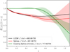 |
Fig. 1. Reconstruction of the expansion rate, E(z)/(1 + z), as a function of the redshift using SNIa data alone. The black line represents the ΛCDM model, while the red band shows the reconstruction with Δχ2 ≤ 1 with respect to the best reconstruction (red line). The green band stands for the reconstruction of a coasting universe at low redshift. See the text for the details of the reconstruction. |
In Table 2 we can clearly see that all the SNIa nuisance-parameter values (α, β, M, ΔM) are compatible for the three models, and that a coasting universe shows a lower expansion rate when we increase the redshift with respect to the standard spline reconstruction. This is confirmed from Fig. 1 where we see that the expansion rate drops above z ≈ 0.8. We can also observe in this figure that the bands increase when we increase the redshift; this is expected since there are less data points in this region. Comparing the three models, we observe that the spline reconstruction provides a slightly smaller χ2 value (681.38) than ΛCDM (682.89), but the former has many more parameters in the model, and so the ability of these models to fit the data is roughly the same, being slightly better for ΛCDM (P( χ2, ν) = 0.915) than the spline reconstruction (P( χ2, ν) = 0.905). However, the χ2 value obtained for the coasting reconstruction (717.60) is much larger than the previous values, which also implies that this model is less able to perfectly fit the data (P( χ2, ν) = 0.661). A detailed model comparison is beyond the scope of this work, since we do not aim to propose a new cosmological model to confront ΛCDM but are interested in studying the accelerated expansion of the universe and the relation it may have with SNIa luminosity. However, the coasting reconstruction has a relative probability of exp(−Δχ2/2)≈1.4 × 10−6%, showing that a coasting universe at low redshift is highly disfavored (>5σ)5, even using SNIa data alone, when SNIa intrinsic luminosity is assumed to be redshift independent. We also note that, even if we ask the reconstruction to be nonaccelerated at low redshift, it prefers to add some acceleration at earlier times (above z ≈ 0.8) rather than simply having a constant velocity expansion.
4.2. Case 2: SNIa+BAO
After having shown how the reconstruction method works, and having applied it to SNIa data alone, we focus on the combination of SNIa and BAO data. As is shown in Table 1 we consider two different ways to combine these data sets: we either let the product H0rd free, or we add a prior on rd. Since we consider the models with and without SNIa intrinsic luminosity evolution, and we always add ΛCDM as a reference, we finally have four different sub-cases with the corresponding three models per sub-case. The best-fit values and errors of the parameters for all these cases are shown in Table 3.
Let us first focus on the case where H0rd is treated as a free parameter. As was the case with SNIa data alone, all the SNIa nuisance parameters (α, β, M, ΔM) have compatible values for the different models considered. However, the coasting reconstruction now does not show a reduced expansion rate at high redshift (adding or not SNIa luminosity evolution), due to the addition of the BAO data points above z ≈ 0.8. We can also see that the value of H0rd obtained from the spline reconstruction is more or less compatible with the one obtained with ΛCDM, but it is lower for the coasting reconstruction, adding SNIa intrinsic luminosity or not. Concerning the ability of the models to fit the data, the χ2 of the spline reconstruction is always slightly smaller than the ΛCDM one (695.65 against 698.06, and 693.21 against 698.06 when we allow the SNIa luminosity to vary). But as was the case before, the probability of providing a good fit is roughly the same for both models, being slightly better for ΛCDM (0.902 against 0.912, and 0.904 for both when we account for evolution). This is also what can be seen in the reconstruction plot on the left panel of Fig. 2. With respect to the coasting reconstruction, we can see in Table 3 that when SNIa intrinsic luminosity is allowed to vary we obtain a χ2 value very close to the ΛCDM one, thus giving also a good probability to correctly fit the data (0.901 against 0.904, for the standard reconstruction, and for ΛCDM).
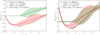 |
Fig. 2. Reconstruction of the expansion rate, E(z)/(1 + z) (left) and H(z)/(1 + z) (right), as a function of the redshift using the combination of SNIa and BAO data. In the left panel the data sets have been combined considering H0rd a free parameter, while in the right panel a prior on rd has been added. In both panels the black and gray lines represent the ΛCDM model (without and with SNIa luminosity evolution, respectively), while the red band shows the reconstruction with Δχ2 ≤ 1 with respect to the best reconstruction (red line). The green band stands for the reconstruction of a coasting universe at low redshift when SNIa intrinsic luminosity is allowed to vary as a function of the redshift. See the text for the details of the reconstruction. |
Best-fit values with the corresponding 1σ error bars for the cosmological and nuisance parameters of the second case: SNIa and BAO data.
Let us now focus on the combination of SNIa and BAO data with a prior on rd (two last rows of Table 3 and the right panel of Fig. 2). This allows us to obtain a constraint on H0, and so we represent in this case the expansion rate by H(z)/(1 + z). All the best-fit values of the parameters are very close to the previous case, with nearly the same χ2 values and the same probabilities, since we have only added one data point and one parameter in the analysis. As before, a coasting universe provides a good fit to the data with a probability of 0.901 against 0.904 for the standard spline reconstruction, and 0.905 for ΛCDM, when SNIa luminosity is allowed to vary. The interesting result from these cases is that the value found for H0 for the spline reconstruction is always smaller than the one obtained for ΛCDM, but still compatible (67.4 ± 1.3 km s−1 Mpc−1 compared to 68.57 ± 0.99 km s−1 Mpc−1, when SNIa luminosity is allowed to vary), while it is significantly smaller for the coasting reconstruction, as can be seen in the right plot of Fig. 2 (62.12 ± 0.56 km s−1 Mpc−1 compared to 68.57 ± 0.99 km s−1 Mpc−1, when SNIa luminosity is allowed to vary). This is consistent with the lower value found for H0rd in the previous cases for the coasting reconstruction.
4.3. Case 3: SNIa+BAO+CMB
Let us recall that the addition of CMB data is a key ingredient when studying cosmological models thanks to its complementarity to low-redshift cosmological probes (see e.g., Tutusaus et al. 2016 where cosmological models are ruled out thanks to the introduction of CMB scale information). Therefore, as a final case we consider the combination of the three main background expansion cosmological probes: SNIa, BAO, and CMB. We have already presented two different ways to combine SNIa and BAO data, so when we add CMB data we keep this approach and, since we now include the physics of the early universe, we add a third way consisting in computing the explicit value of rd. The best-fit values of the parameters for these three sub-cases are presented in Table 4 with the 1σ errors, and the corresponding reconstruction is shown in Fig. 3. Let us mention that even if zCMB and zdrag in Table 4 seem to be fixed, both of them have been fitted each time adding the Planck priors; however, the best-fit values are very stable and are identical in the table given the number of decimals presented.
Best-fit values with the corresponding 1σ error bars for the cosmological and nuisance parameters of the third case: SNIa, BAO, and CMB data.
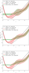 |
Fig. 3. Reconstruction of the expansion rate, H(z)/(1 + z), as a function of the redshift using the combination of SNIa, BAO, and CMB data. In the top panel the data sets have been combined considering rd a free parameter, while in the central panel a prior on rd has been used, and it has been explicitly computed in the bottom panel. In all panels the black and gray lines represent the ΛCDM model (without and with SNIa luminosity evolution, respectively), while the red band shows the reconstruction with Δχ2 ≤ 1 with respect to the best reconstruction (red line). The green band stands for the reconstruction of a coasting universe at low redshift when SNIa intrinsic luminosity is allowed to vary as a function of redshift. See the text for the details of the reconstruction. |
Let us start with the combination considering rd a free parameter. Either assuming the SNIa intrinsic luminosity to be redshift independent or allowing it to vary, the three models provide compatible values for all the parameters except H0, which is significantly smaller for the coasting reconstruction, as was already shown in the combination of SNIa and BAO data, and which is compensated by a larger Ωm. We note that the CMB is sensitive to the physical matter energy density Ωmh2, which is roughly equal to 0.14 for all models. Therefore, even if the value of H0 is smaller than in the concordance model, if the value of Ωm is large enough, the coasting reconstruction can also perfectly fit the CMB. When SNIa luminosity is allowed to vary, a coasting reconstruction provides roughly the same χ2 (698.30) as ΛCDM (698.09) with a slightly smaller probability (0.898 against 0.908), showing that a nonaccelerated expanding universe can fit the three main background probes when SNIa intrinsic luminosity is allowed to vary.
In a second place we add a prior on rd (Verde et al. 2017b) obtained without assumptions on the late-time universe. All the best-fit values are compatible between the different models as before, except for H0 and Ωm, which are smaller and larger for a coasting reconstruction, respectively, accounting for SNIa luminosity evolution or not. The obtained χ2 values are very similar, leading to very similar probabilities to correctly fit the data, P(χ2, ν), and they show that a coasting reconstruction can correctly fit the data when SNIa luminosity evolution is accounted for. In the last place we compute rd using Eq. (5). All the best-fit values are compatible with the previous results, and compatible between the different models, except for H0 and Ωm. It is also the case for the χ2 values and the corresponding probabilities.
We conclude that, if we account for a redshift dependence in the intrinsic luminosity of SNIa, the main cosmological probes cannot firmly prove the accelerated nature of the expansion of the universe in a model-independent way, since a nonaccelerated reconstruction of the expansion rate can correctly fit the observations.
For completeness, we present in Fig. 4 the residuals to SNIa and BAO observations for three different models: ΛCDM (black), the reconstruction through cubic splines (red), and the nonaccelerated model using a coasting reconstruction (green) taking into account SNIa intrinsic luminosity evolution. We also provide the predictions for the CMB quantities R, ℓa, and ωb in Table 5. All these predictions have been computed using the best-fit values of the parameters obtained from the global fit to the combination of SNIa, BAO, and CMB data, explicitly computing the value of rd using Eq. (5). From these results we can see graphically that all three models are perfectly able to fit the data; including the coasting reconstruction with SNIa luminosity evolution. As can be seen in Table 4, a different approach when combining SNIa, BAO, and CMB data (free rd or prior on rd) gives nearly the same values for the parameters of the reconstruction, which leads to almost the same predictions for the observables.
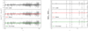 |
Fig. 4. Residuals between the observations and the prediction of the different models, ΛCDM, spline reconstruction, and coasting reconstruction with SNIa intrinsic luminosity evolution, for the SNIa and BAO observables. The predictions have been computed using the best-fit values for the parameters obtained from the fit of the combination SNIa+BAO+CMB computing rd explicitly. Left plot: residuals of the SNIa distance modulus for the three different models: ΛCDM (black, top panel), spline reconstruction (red, central panel), and coasting reconstruction (green, bottom panel). The residuals have been normalized with respect to the prediction for each model. Right plot: residuals of the BAO measurements following the same color convention as in the left panel. The residuals have been normalized with respect to the prediction for each model. |
Prediction of the different models for the CMB quantities R, ℓa, ωb, for the combination of SNIa, BAO, and CMB data computing rd explicitly, and accounting for SNIa intrinsic luminosity evolution as a function of the redshift when dealing with a coasting reconstruction.
4.4. Pantheon SNIa sample
Although our main cosmological data set for SNIa measurements in this analysis is the JLA compilation from Betoule et al. (2014), there is a newer compilation available in the community called Pantheon (Scolnic et al. 2018). It contains SNIa measurements coming from the Pan-STARRS1 Medium Deep Survey, SDSS, SNLS, various low-redshift surveys, and HST samples. Pantheon is the largest combined sample of SNIa with a total amount of 1048 SNIa from z = 0.01 up to z = 2.3. Besides the increased number of SNIa compared to JLA (740), and the extended redshift range (z ≈ 1 for JLA), the Pantheon compilation considers a different treatment of SNIa systematic errors. For instance, the mass step ΔM, α, and β nuisance parameters appearing in the JLA compilation are here pre-solved in a cosmology independent manner (see Scolnic et al. 2018 for the details), so the Pantheon compilation provides only the redshifts, distance moduli, and distance moduli uncertainties, together with the covariance matrix for the distances moduli. A detailed comparison between the different treatment of systematic errors between these two compilations is beyond the scope of this work.
Our interest here is to test the stability of our results from the previous section when using the Pantheon sample instead of the JLA compilation. In order to do this, we reconstruct the expansion rate for case 3: SNIa+BAO+CMB, computing rd explicitly and replacing the JLA compilation with the Pantheon one. The results are shown in Fig. 5 and they should be compared to the bottom panel of Fig. 3. As can be seen from the comparison of the figures (and the χ2/d.o.f. values quoted in them), our main results from the previous section remain qualitatively unaltered. The coasting reconstruction, when SNIa intrinsic luminosity is allowed to vary as a function of the redshift, is able to provide a very good fit to the main background cosmological probes. It is important to mention however that the Δχ2 between the coasting reconstruction in Fig. 3 (JLA) and the concordance model is equal to −0.3 (smaller for the coasting reconstruction), while the Δχ2 when considering the Pantheon compilation is equal to 4.3 (smaller for the concordance model). Although this difference is not large enough to rule out the coasting reconstruction, it already shows some tension; therefore, it might point towards the fact that with future SNIa compilations, with even higher sample sizes, we might be able to discard this kind of reconstruction. It is also interesting to note that the reduced χ2/d.o.f. are always smaller than 1 when considering the Pantheon compilation, but they are slightly larger than the ones obtained with the JLA compilation. This is probably due to the different treatment of systematic errors in the different compilations; however, all models provide a very good fit to the data and a detailed comparison on the treatment of systematic errors is beyond the scope of this work.
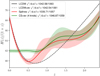 |
Fig. 5. Reconstruction of the expansion rate, H(z)/(1 + z), as a function of the redshift using the combination of SNIa, BAO, and CMB data, explicitly computing the value of rd. In this case the Pantheon compilation of SNIa has been used instead of the JLA compilation. The black and gray lines represent the ΛCDM model (without and with SNIa luminosity evolution, respectively), while the red band shows the reconstruction with Δχ2 ≤ 1 with respect to the best reconstruction (red line). The green band stands for the reconstruction of a coasting universe at low redshift when SNIa intrinsic luminosity is allowed to vary as a function of redshift. See text for details of the reconstruction. |
4.5. Growth rate
The measurements of the growth rate of matter perturbations offer an additional constraint on cosmological models. Their values depend on the theory of gravity used and it is well known that there are identical background evolutions with different growth rates (Piazza et al. 2014). Defining the linear growth factor of matter perturbations as the ratio between the linear density perturbation and the energy density, D ≡ δρm/ρm, we can derive the standard second-order differential equation for D (Peebles 1993)
 (16)
(16)
where the dot stands for differentiation over cosmic time. Neglecting second-order corrections, this differential equation can be rewritten with derivatives over the scale factor (Dodelson 2003)
![Mathematical equation: $$ \begin{aligned} D^{\prime \prime }(a)+\left[\frac{3}{a}+\frac{H^{\prime }(a)}{H(a)}\right]D^{\prime }(a)-\frac{3}{2}\Omega _{\rm m}\frac{H_0^2}{H^2(a)}\frac{D(a)}{a^5}=0, \end{aligned} $$](/articles/aa/full_html/2019/05/aa33032-18/aa33032-18-eq22.gif) (17)
(17)
which is valid under the assumption that dark energy cannot be perturbed and does not interact with dark matter. We can now define the growth rate as
 (18)
(18)
and then compute the observable weighted growth rate f σ8 as
 (19)
(19)
where σ8Planck stands for the ΛCDM observed value (with Planck) of the root mean square mass fluctuation amplitude on scales of 8h−1 Mpc at redshift z = 0 (fixed to 0.8159 in this work Planck Collaboration XIII 2016), and DPlanck represents the ΛCDM Planck growth factor (Planck Collaboration XIII 2016). In this work we consider the measurements of the weighted growth rate from the 6dFGS survey (Beutler et al. 2012), the WiggleZ survey (Blake et al. 2012), and the VIPERS survey (de la Torre et al. 2013), as well as the different SDSS projects: SDSS-II MGS DR7 (Howlett et al. 2015; with the main galaxy sample of the seventh data release), SDSS-III BOSS DR12 (Alam et al. 2017; with the LRGs from the twelfth BOSS data release), and SDSS-IV DR14Q (Gil-Marín et al. 2018; with the latest quasar sample of eBOSS). We have not included this data set in our fitting analysis for simplicity, but we show in Fig. 6 that when using the best-fit values of the parameters from the SNIa+BAO+CMB fit the prediction for the three models considered (ΛCDM, spline reconstruction, and coasting reconstruction with SNIa luminosity evolution) is in very good agreement with the observations. We note that the values for the parameters used in Fig. 6 have been obtained computing the value of rd, but the results are equivalent using the other approaches for the combination of our three main data sets.
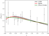 |
Fig. 6. Prediction of the different models, ΛCDM, spline reconstruction, and coasting reconstruction with SNIa intrinsic luminosity evolution, for the growth of matter perturbations f σ8 observable. The predictions have been computed using the best-fit values for the parameters obtained from the fit of the combination SNIa+BAO+CMB computing rd explicitly. Therefore, it is not a fit to the f σ8 measurements. We follow the same color legend as in the previous figures: black for ΛCDM, red for the spline reconstruction, and green for the coasting reconstruction. |
4.6. The Hubble constant
The Hubble constant, H0, is one of the most important parameters in modern cosmology, since it is used to construct time and distance cosmological scales. It was first measured by Hubble to be roughly 500 km s−1 Mpc−1 (Hubble 1929). Current data supports a value for H0 close to 70 km s−1 Mpc−1. However, nearly 100 years later there is still no consensus on its value. Local measurements already show some tension on the results depending on the calibration of SNIa distances and the methodology used. Using median statistics, the authors from Gott et al. (2001), Chen et al. (2003), and Chen & Ratra (2011) finally found a local value of H0 equal to 68 ± 5.5 km s−1 Mpc−1 (95% statistical and systematic errors). Following these studies, there were different analyses claiming values close to 68 km s−1 Mpc−1 using different methods and assumptions (see e.g., Chen et al. 2017; Yu et al. 2018; Rigault et al. 2015; Zhang et al. 2017; Dhawan et al. 2018; Fernández Arenas et al. 2018; Lin & Ishak 2017, and Haridasu et al. 2018b). However, there are other studies claiming significantly higher values (Riess et al. 2018b,c, 2016), and some others finding slightly smaller values (Tammann & Reindl 2013). Moreover, there is also some tension between some direct measurements of H0 and the value inferred from the CMB assuming a ΛCDM model (Planck Collaboration XIII 2016). There have been many attempts in the literature to solve this discrepancy both from an observational and a theoretical perspective (see Bernal et al. 2016; Gómez-Valent & Amendola 2018; Mörtsell & Dhawan 2018; Dhawan et al. 2018; Ben-Dayan et al. 2014; D’Arcy Kenworthy et al. 2019; Shanks et al. 2019; Riess et al. 2018d, and references therein for a detailed discussion on the trouble with H0). In this work we consider two recent cosmological model-independent measurements of H0 in order to check its effect on the conclusions we can draw concerning cosmic acceleration. We first consider the value obtained from the Hubble Space Telescope observations (Riess et al. 2018b; R18 in the following), H0 = 73.45 ± 1.66 km s−1 Mpc−1. We then consider the value obtained with Gaussian processes using SNIa data, and constraints on H(z) from cosmic chronometers (Gómez-Valent & Amendola 2018; GVA18 in the following), H0 = 67.06 ± 1.68 km s−1 Mpc−1. This last value is closer to the one derived with an “inverse distance ladder” approach in Aubourg et al. (2015), H0 = 67.3 ± 1.1, where the measurement assumes standard pre-recombination physics but is insensitive to dark energy or space curvature assumptions. It is also closer to the value derived from the CMB observations using a flat ΛCDM model, H0 = 67.51 ± 0.64 (Planck Collaboration XIII 2016).
Let us mention that in this work we also provide constraints on H0 obtained using a cubic spline reconstruction on SNIa, BAO, and CMB data without SNIa intrinsic luminosity evolution (as in GVA18). They are given by H0 = 68.5 ± 1.7 (free rd), H0 = 68.3 ± 1.2 (prior rd), and H0 = 68.2 ± 1.2 (compute rd). See Table 4 for the constraints including SNIa luminosity evolution. All our constraints are compatible (within 1σ) with GVA18 and Planck but they are in tension with R18. However, we keep R18 and GVA18 in the following to use H0 constraints, without assumptions on the cosmological model, which are independent from this work.
In Fig. 7 we represent the profile likelihood (assuming Gaussian likelihoods) for both the observed values of H0, R18 (black) and GVA18 (blue), and the values derived from the nonaccelerated reconstruction for the combination SNIa+BAO+CMB taking into account the SNIa intrinsic luminosity evolution. We present the three values obtained for the three approaches followed when combining the data sets: considering rd a free parameter (green), adding a prior on it (yellow), or computing it explicitly (purple). From the figure alone it is clear that the H0 value for the nonaccelerated reconstruction is in tension with R18 at more than 5σ, independently of the approach used when combining the data sets. More precisely, a nonaccelerated reconstruction is ruled out if we consider the R18 measurement at 5.60σ (free rd, H0 = 62.2 ± 1.1), 6.47σ (prior rd, H0 = 62.13 ± 0.55), or 6.55σ (compute rd, H0 = 62.08 ± 0.51), showing that, with the R18 measurement, cosmic acceleration is proven even if some astrophysical systematic errors evolving with the redshift modify the intrinsic luminosity of SNIa. However, we can also see from the figure that if we consider the measured value from the Gaussian processes, a nonaccelerated reconstruction shows slightly less than a 3σ tension. More precisely, there is a tension of 2.39σ (free rd), 2.79σ (prior rd), or 2.84σ (compute rd). In this case, the measured value of H0 points towards ruling out these reconstructions, but the tension is still far from the usually recognized 5σ threshold.
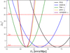 |
Fig. 7. Profile likelihood (minus |

Before moving on to our conclusions, let us mention that there have been several analyses in the literature where the authors constrain the expansion rate of the universe, H(z), using measurements of it. Different cosmological models or reconstruction methods have been used (see e.g., Farooq & Ratra 2013; Farooq et al. 2017, 2013; Moresco et al. 2016, and Yu et al. 2018). Using local measurements of H0, these analyses also show current acceleration and earlier deceleration, which enables us to obtain the redshift of transition between deceleration and acceleration. In order to compare our results to theirs, we compute this transition redshift for the different (noncoasting) spline reconstructions. For SNIa alone, the redshift of transition is zt = 0.9 ± 1.2, given the lack of constraining power from SNIa data alone. However, when we include BAO data this transition becomes zt = 0.55 ± 0.32 (free H0rd) and zt = 0.54 ± 0.25 (prior on rd). If we also add CMB data into the analysis, the transition redshift is then given by zt = 0.53 ± 0.33 (free rd), zt = 0.53 ± 0.24 (prior rd), and zt = 0.53 ± 0.24 (compute rd). These results are compatible with the transition redshift derived in a model-independent way in Moresco et al. (2016): zt = 0.4 ± 0.1, as well as the value derived using median statistics in Farooq et al. (2017): zt = 0.74 ± 0.05. Therefore, our cubic spline reconstructions (without SNIa intrinsic luminosity evolution) provide information on the transition from deceleration to acceleration compatible to that obtained with H(z) and H0 data.
5. Conclusions
Here we address the question of whether or not relaxing the standard assumption that SNIa intrinsic luminosity does not depend on the redshift can have an impact on the conclusions that can be drawn on the accelerated nature of the expansion of the universe. Although there is no theoretically fully motivated model for this luminosity evolution yet, it has not been proven that two SNIa in two galaxies with the same light curve, color, and host stellar mass have the same intrinsic luminosity independently of redshift. Moreover, there are different studies claiming a detection of SNIa luminosity dependence on the star formation rate or metallicity of the host galaxy, which depend on the redshift (Rigault et al. 2013, 2017; Childress et al. 2014; Moreno-Raya et al. 2016). Also, with this kind of analysis we can distinguish between the effect of unknown astrophysical systematics varying with the redshift and the cosmological information.
The impact of SNIa luminosity evolution on our cosmological knowledge has already been addressed (Wright 2002; Drell et al. 2000; Linden et al. 2009; Nordin et al. 2008; Ferramacho et al. 2009; Tutusaus et al. 2016, 2017; L’Huillier et al. 2019), but in this work we have extended the analysis by including the physics of the early universe (z ≈ 1000), and consider the main background cosmological probes: SNIa, BAO, and the CMB. In order to maximise the scope of this study, we have not imposed a cosmological model, but we have reconstructed the expansion rate of the universe using a cubic spline interpolation.
We first applied, as an illustration of the method, the reconstruction to SNIa data alone with the standard assumption of SNIa luminosity independence. We have shown that with this assumption cosmic acceleration is definitely preferred against a local nonaccelerated universe.
In a second step we added the latest BAO data to our analysis. We considered two different ways to combine it with SNIa data: either we considered H0rd as a free parameter, or we added a prior on rd coming from CMB observations, without any dependence on late-time universe assumptions. In both cases we see that a nonaccelerated universe is able to fit the data nearly as well as ΛCDM, when we allow the SNIa intrinsic luminosity to vary as a function of the redshift.
Subsequently, we extended the data sets in the analysis by adding the information coming from the CMB through the reduced parameters. In order to deal with this information we were forced to specify the model up to very high redshifts. We decided to follow a matter–radiation-dominated model from the early universe down to z ≈ 3, where we start to have low-redshift data. We then coupled the model to our spline reconstruction. In other words, we considered a matter–radiation-dominated model at the early universe and, when we entered the redshift range where we have low-redshift data and a cosmological constant is still negligible, we allowed the expansion rate to vary freely without specifying any dark energy model. When adding the CMB data we followed three different approaches: treat rd as a free parameter, add a prior on it, or compute it assuming that the BAO and the CMB share the same physics. For simplicity we did not add the f σ8 measurements of the growth rate of matter perturbations, but we checked that when using the best-fit values from the global fit SNIa+BAO+CMB we were able to correctly predict the latest f σ8 measurements.
In all three cases we have seen that a nonaccelerated model is able to nicely fit the main background cosmological probes, when SNIa intrinsic luminosity is allowed to vary as a function of the redshift, including the information on the early universe coming from the CMB.
After this conclusion, we focus on the impact that the Hubble constant may have on this question. We considered two different recent model-independent measurements of H0: 73.45 ± 1.66 km s−1 Mpc−1 (R18) from Riess et al. (2018b), and 67.06 ± 1.68 km s−1 Mpc−1 (GVA18) from Gómez-Valent & Amendola (2018). We showed that if we consider the R18 value, cosmic acceleration is proven at more than 5.60σ for a general expansion rate reconstruction (for which we get H0 = 62.2 ± 1.1 (free rd), H0 = 62.13 ± 0.55 (prior rd), and H0 = 62.08 ± 0.51 (compute rd)), even if SNIa intrinsic luminosity varies as a function of the redshift due to some astrophysical unknown systematic error. It is important to mention, however, that if we consider the GVA18 value, a nonaccelerated reconstruction for the expansion rate is at a 3σ tension with the measurement, but still below the 5σ detection.
In conclusion, if SNIa intrinsic luminosity varies as a function of the redshift, a nonaccelerated universe is able to correctly fit all the main background probes. However, the value of H0 turns out to be a key ingredient in the conclusions we can draw concerning cosmic acceleration. If we take H0 into account we are close to claiming an accelerated expansion of the universe using an approach that is very independent of the cosmological model assumed, and even if SNIa intrinsic luminosity varies as a function of the redshift. A final consensus on a direct measurement of H0 and its precision will be decisive in finally proving the cosmic acceleration independently of the cosmological model and any redshift dependent astrophysical systematic error that may remain in the SNIa analysis.
These values have been chosen such that the expansion rate has a significant amount of freedom at low redshift, and because this is the interval for which SNIa data are available.
This corresponds to the redshift of the Ly-α forest measurements.
When using SNIa data alone we only fix the first three knots because there is not a lot of data beyond z ∼ 0.8, but we have checked that fixing the first four knots leads to equivalent conclusions.
We note that we do find more than a 5σ preference for cosmic acceleration (when SNIa luminosity does not evolve with the redshift), contrary to the results of Nielsen et al. (2016), because we consider the standard SNIa systematics instead of the extra systematics proposed by these authors. However, we are still far from the 11.2σ detection from Rubin & Hayden (2016), because we use a model-independent reconstruction with many more degrees of freedom than a fixed nonaccelerated model.
Acknowledgments
We thank Adam G. Riess and Daniel L. Shafer for very fruitful comments which helped to noticeably improve this work. This work has been carried out thanks to the support of the OCEVU Labex (ANR-11-LABX-0060) and of the Excellence Initiative of Aix-Marseille University - A*MIDEX, part of the French “Investissements d’Avenir” programme. IT acknowledges support from the Spanish Ministry of Science, Innovation and Universities through grant ESP2017-89838-C3-1-R, and the H2020 programme of the European Commission through grant 776247.
References
- Alam, S., Ata, M., Bailey, S., et al. 2017, MNRAS, 470, 2617 [NASA ADS] [CrossRef] [Google Scholar]
- Aubourg, E., Bailey, S., Bautista, J. E., et al. 2015, Phys. Rev. D, 92, 123516 [NASA ADS] [CrossRef] [Google Scholar]
- Bassett, B. A., & Afshordi, N. 2010, ArXiv e-prints [arXiv:1005.1664] [Google Scholar]
- Bautista, J. E., Busca, N. G., Guy, J., et al. 2017, A&A, 603, A12 [NASA ADS] [CrossRef] [EDP Sciences] [Google Scholar]
- Ben-Dayan, I., Durrer, R., Marozzi, G., & Schwarz, D. J. 2014, Phys. Rev. Lett., 112, 221301 [NASA ADS] [CrossRef] [PubMed] [Google Scholar]
- Bernal, J. L., Verde, L., & Riess, A. G. 2016, JCAP, 10, 019 [NASA ADS] [CrossRef] [Google Scholar]
- Betoule, M., Kessler, R., Guy, J., et al. 2014, A&A, 568, A22 [NASA ADS] [CrossRef] [EDP Sciences] [Google Scholar]
- Beutler, F., Blake, C., Colless, M., et al. 2011, MNRAS, 416, 3017 [NASA ADS] [CrossRef] [Google Scholar]
- Beutler, F., Blake, C., Colless, M., et al. 2012, MNRAS, 423, 3430 [NASA ADS] [CrossRef] [Google Scholar]
- Blake, C., Brough, S., Colless, M., et al. 2012, MNRAS, 425, 405 [NASA ADS] [CrossRef] [Google Scholar]
- Busti, V. C., Clarkson, C., & Seikel, M. 2014, MNRAS, 441, L11 [NASA ADS] [CrossRef] [Google Scholar]
- Chen, G., & Ratra, B. 2011, PASP, 123, 1127 [NASA ADS] [CrossRef] [Google Scholar]
- Chen, G., Gott, J., Richard, I., & Ratra, B. 2003, PASP, 115, 1269 [NASA ADS] [CrossRef] [Google Scholar]
- Chen, Y., Kumar, S., & Ratra, B. 2017, ApJ, 835, 86 [NASA ADS] [CrossRef] [Google Scholar]
- Childress, M. J., Wolf, C., & Zahid, H. J. 2014, MNRAS, 445, 1898 [NASA ADS] [CrossRef] [Google Scholar]
- Clarkson, C., & Zunckel, C. 2010, Phys. Rev. Lett., 104, 211301 [NASA ADS] [CrossRef] [PubMed] [Google Scholar]
- Colin, J., Mohayaee, R., Rameez, M., & Sarkar, S. 2018, ArXiv e-prints [arXiv:1808.04597] [Google Scholar]
- Crittenden, R. G., Pogosian, L., & Zhao, G.-B. 2009, JCAP, 12, 025 [NASA ADS] [CrossRef] [Google Scholar]
- Dam, L. H., Heinesen, A., & Wiltshire, D. L. 2017, MNRAS, 472, 835 [NASA ADS] [CrossRef] [Google Scholar]
- D’Arcy Kenworthy, W., Scolnic, D., & Riess, A. 2019, ApJ, in press [arXiv:1901.08681] [Google Scholar]
- de la Torre, S., Guzzo, L., Peacock, J. A., et al. 2013, A&A, 557, A54 [NASA ADS] [CrossRef] [EDP Sciences] [Google Scholar]
- Dhawan, S., Jha, S. W., & Leibundgut, B. 2018, A&A, 609, A72 [NASA ADS] [CrossRef] [EDP Sciences] [Google Scholar]
- Dodelson, S. 2003, Modern Cosmology (Academic Press) [Google Scholar]
- Drell, P. S., Loredo, T. J., & Wasserman, I. 2000, ApJ, 530, 593 [NASA ADS] [CrossRef] [Google Scholar]
- du Mas des Bourboux, H., Le Goff, J. M., Blomqvist, M., et al. 2017, A&A, 608, A130 [NASA ADS] [CrossRef] [EDP Sciences] [Google Scholar]
- Eisenstein, D. J., & Hu, W. 1998, ApJ, 496, 605 [NASA ADS] [CrossRef] [Google Scholar]
- Farooq, O., & Ratra, B. 2013, ApJ, 766, L7 [NASA ADS] [CrossRef] [MathSciNet] [Google Scholar]
- Farooq, O., Crandall, S., & Ratra, B. 2013, Phys. Lett. B, 726, 72 [NASA ADS] [CrossRef] [Google Scholar]
- Farooq, O., Ranjeet Madiyar, F., Crandall, S., & Ratra, B. 2017, ApJ, 835, 26 [NASA ADS] [CrossRef] [Google Scholar]
- Fernández Arenas, D., Terlevich, E., Terlevich, R., et al. 2018, MNRAS, 474, 1250 [NASA ADS] [CrossRef] [Google Scholar]
- Ferramacho, L. D., Blanchard, A., & Zolnierowski, Y. 2009, A&A, 499, 21 [NASA ADS] [CrossRef] [EDP Sciences] [Google Scholar]
- Fixsen, D. J. 2009, ApJ, 707, 916 [Google Scholar]
- Gil-Marín, H., Guy, J., Zarrouk, P., et al. 2018, MNRAS, 477, 1604 [NASA ADS] [CrossRef] [Google Scholar]
- Gómez-Valent, A. 2018, ArXiv e-prints [arXiv:1810.02278] [Google Scholar]
- Gómez-Valent, A., & Amendola, L. 2018, JCAP, 2018, 051 [CrossRef] [Google Scholar]
- Goobar, A., Dhawan, S., & Scolnic, D. 2018, MNRAS, 477, L75 [NASA ADS] [CrossRef] [Google Scholar]
- Gott, J., Richard, I., Vogeley, M. S., Podariu, S., & Ratra, B. 2001, ApJ, 549, 1 [NASA ADS] [CrossRef] [Google Scholar]
- Haridasu, B. S., Luković, V. V., D’Agostino, R., & Vittorio, N. 2017, A&A, 600, L1 [NASA ADS] [CrossRef] [EDP Sciences] [Google Scholar]
- Haridasu, B. S., Luković, V. V., Moresco, M., & Vittorio, N. 2018a, JCAP, 2018, 015 [CrossRef] [Google Scholar]
- Haridasu, B. S., Luković, V. V., & Vittorio, N. 2018b, JCAP, 2018, 033 [CrossRef] [Google Scholar]
- Holsclaw, T., Alam, U., Sansó, B., et al. 2010, Phys. Rev. D, 82, 103502 [NASA ADS] [CrossRef] [Google Scholar]
- Hou, J., Sánchez, A. G., Scoccimarro, R., et al. 2018, MNRAS, 480, 2521 [Google Scholar]
- Howlett, C., Ross, A. J., Samushia, L., Percival, W. J., & Manera, M. 2015, MNRAS, 449, 848 [NASA ADS] [CrossRef] [Google Scholar]
- Hubble, E. 1929, Proc. Nat. Acad. Sci., 15, 168 [NASA ADS] [CrossRef] [Google Scholar]
- Huterer, D., & Starkman, G. 2003, Phys. Rev. Lett., 90, 031301 [NASA ADS] [CrossRef] [PubMed] [Google Scholar]
- James, F., & Roos, M. 1975, Comput. Phys. Commun., 10, 343 [NASA ADS] [CrossRef] [PubMed] [Google Scholar]
- Johansson, J., Thomas, D., Pforr, J., et al. 2013, MNRAS, 435, 1680 [NASA ADS] [CrossRef] [Google Scholar]
- Jones, D. O., Riess, A. G., Scolnic, D. M., et al. 2018, ApJ, 867, 108 [NASA ADS] [CrossRef] [Google Scholar]
- L’Huillier, B., & Shafieloo, A. 2017, JCAP, 2017, 015 [Google Scholar]
- L’Huillier, B., Shafieloo, A., & Kim, H. 2018, MNRAS, 476, 3263 [NASA ADS] [CrossRef] [Google Scholar]
- L’Huillier, B., Shafieloo, A., Linder, E. V., & Kim, A. G. 2019, MNRAS, 485, 2783 [NASA ADS] [CrossRef] [Google Scholar]
- Lin, W., & Ishak, M. 2017, Phys. Rev. D, 96, 083532 [NASA ADS] [CrossRef] [Google Scholar]
- Lin, H.-N., Li, X., & Sang, Y. 2018, Chin. Phys. C, 42, 095101 [NASA ADS] [CrossRef] [Google Scholar]
- Linden, S., Virey, J.-M., & Tilquin, A. 2009, A&A, 506, 1095 [NASA ADS] [CrossRef] [EDP Sciences] [Google Scholar]
- Liu, Z.-E., Yu, H.-R., Zhang, T.-J., & Tang, Y.-K. 2016, Phys. Dark Universe, 14, 21 [NASA ADS] [CrossRef] [Google Scholar]
- Lonappan, A. I., Kumar, S., Ruchika, Dinda B. R., & Sen, A. A., 2018, Phys. Rev. D, 97, 043524 [NASA ADS] [CrossRef] [Google Scholar]
- Luković, V. V., Haridasu, B. S., & Vittorio, N. 2018, Found. Phys., 48, 1446 [NASA ADS] [CrossRef] [Google Scholar]
- Moreno-Raya, M. E., Mollá, M., López-Sánchez, Á. R., et al. 2016, ApJ, 818, L19 [NASA ADS] [CrossRef] [Google Scholar]
- Moresco, M., Pozzetti, L., Cimatti, A., et al. 2016, JCAP, 2016, 014 [NASA ADS] [CrossRef] [Google Scholar]
- Mörtsell, E., & Dhawan, S. 2018, JCAP, 2018, 025 [Google Scholar]
- Nielsen, J. T., Guffanti, A., & Sarkar, S. 2016, Nat. Sci. Rep., 6, 35596 [NASA ADS] [CrossRef] [PubMed] [Google Scholar]
- Nordin, J., Goobar, A., & Jönsson, J. 2008, JCAP, 02, 008 [CrossRef] [Google Scholar]
- Peebles, P. 1993, Principles of Physical Cosmology (Princeton University Press) [Google Scholar]
- Penna-Lima, M., Vitenti, S. D. P., Alves, M. E. S., de Araujo, J. C. N., & Carvalho, F. C. 2019, Eur. Phys. J. C, 79, 175 [NASA ADS] [CrossRef] [EDP Sciences] [Google Scholar]
- Perlmutter, S., Aldering, G., Goldhaber, G., et al. 1999, ApJ, 517, 565 [NASA ADS] [CrossRef] [Google Scholar]
- Piazza, F., Steigerwald, H., & Marinoni, C. 2014, JCAP, 05, 043 [CrossRef] [Google Scholar]
- Planck Collaboration XIII. 2016, A&A, 594, A13 [NASA ADS] [CrossRef] [EDP Sciences] [Google Scholar]
- Planck Collaboration XIV. 2016, A&A, 594, A14 [NASA ADS] [CrossRef] [EDP Sciences] [Google Scholar]
- Qin, H. F., Li, X. B., Wan, H. Y., & Zhang, T. J. 2015, ArXiv e-prints [arXiv:1501.02971] [Google Scholar]
- Riess, A. G., Filippenko, A. V., Challis, P., et al. 1998, AJ, 116, 1009 [NASA ADS] [CrossRef] [Google Scholar]
- Riess, A. G., Macri, L. M., Hoffmann, S. L., et al. 2016, ApJ, 826, 56 [NASA ADS] [CrossRef] [Google Scholar]
- Riess, A. G., Rodney, S. A., Scolnic, D. M., et al. 2018a, ApJ, 853, 126 [NASA ADS] [CrossRef] [Google Scholar]
- Riess, A. G., Casertano, S., Yuan, W., et al. 2018b, ApJ, 855, 136 [NASA ADS] [CrossRef] [Google Scholar]
- Riess, A. G., Casertano, S., Yuan, W., et al. 2018c, ApJ, 861, 126 [Google Scholar]
- Riess, A. G., Casertano, S., Kenworthy, D., Scolnic, D., & Macri, L. 2018d, ArXiv e-prints [arXiv:1810.03526] [Google Scholar]
- Rigault, M., Copin, Y., Aldering, G., et al. 2013, A&A, 560, A66 [NASA ADS] [CrossRef] [EDP Sciences] [Google Scholar]
- Rigault, M., Aldering, G., Kowalski, M., et al. 2015, ApJ, 802, 20 [NASA ADS] [CrossRef] [Google Scholar]
- Rigault, M., Brinnel, V., Aldering, G., et al. 2017, A&A, submitted [arXiv:1806.03849] [Google Scholar]
- Ringermacher, H. I., & Mead, L. R. 2016, ArXiv e-prints [arXiv:1611.00999] [Google Scholar]
- Ross, A. J., Samushia, L., Howlett, C., et al. 2015, MNRAS, 449, 835 [NASA ADS] [CrossRef] [Google Scholar]
- Rubin, D., & Hayden, B. 2016, ApJ, 833, L30 [NASA ADS] [CrossRef] [PubMed] [Google Scholar]
- Said, N., Baccigalupi, C., Martinelli, M., Melchiorri, A., & Silvestri, A. 2013, Phys. Rev. D, 88, 043515 [NASA ADS] [CrossRef] [Google Scholar]
- Scolnic, D. M., Jones, D. O., Rest, A., et al. 2018, ApJ, 859, 101 [NASA ADS] [CrossRef] [Google Scholar]
- Seikel, M., & Schwarz, D. J. 2008, JCAP, 2008, 007 [NASA ADS] [CrossRef] [Google Scholar]
- Seikel, M., & Schwarz, D. J. 2009, JCAP, 2009, 024 [NASA ADS] [CrossRef] [Google Scholar]
- Seikel, M., Clarkson, C., & Smith, M. 2012, JCAP, 06, 036 [NASA ADS] [CrossRef] [Google Scholar]
- Shafieloo, A. 2007, MNRAS, 380, 1573 [NASA ADS] [CrossRef] [Google Scholar]
- Shanks, T., Hogarth, L. M., & Metcalfe, N. 2019, MNRAS, 484, L64 [NASA ADS] [CrossRef] [Google Scholar]
- Shariff, H., Jiao, X., Trotta, R., & van Dyk, D. A. 2016, ApJ, 827, 1 [NASA ADS] [CrossRef] [Google Scholar]
- Starobinsky, A. A., Shafieloo, A., Alam, U., & Sahni, V. 2006, MNRAS, 366, 1081 [NASA ADS] [CrossRef] [Google Scholar]
- Sullivan, M., Guy, J., Conley, A., et al. 2011, ApJ, 737, 102 [NASA ADS] [CrossRef] [Google Scholar]
- Tammann, G. A., & Reindl, B. 2013, A&A, 549, A136 [NASA ADS] [CrossRef] [EDP Sciences] [Google Scholar]
- Tripp, R. 1998, A&A, 331, 815 [NASA ADS] [Google Scholar]
- Tutusaus, I., Lamine, B., Blanchard, A., et al. 2016, Phys. Rev. D, 94, 103511 [NASA ADS] [CrossRef] [Google Scholar]
- Tutusaus, I., Lamine, B., Dupays, A., & Blanchard, A. 2017, A&A, 602, A73 [NASA ADS] [CrossRef] [EDP Sciences] [Google Scholar]
- Verde, L., Bernal, J. L., Heavens, A. F., & Jimenez, R. 2017a, MNRAS, 467, 731 [NASA ADS] [Google Scholar]
- Verde, L., Bellini, E., Pigozzo, C., Heavens, A. F., & Jimenez, R. 2017b, JCAP, 04, 023 [NASA ADS] [CrossRef] [Google Scholar]
- Vitenti, S. D. P., & Penna-Lima, M. 2015, JCAP, 9, 045 [NASA ADS] [CrossRef] [Google Scholar]
- Wang, D., & Meng, X. 2017, Mech. Astron., 60, 110411 [CrossRef] [Google Scholar]
- Wang, Y., & Mukherjee, P. 2007, Phys. Rev. D, 76, 103533 [NASA ADS] [CrossRef] [Google Scholar]
- Wright, E. L. 2002, ArXiv e-prints [arXiv:astro-ph/0201196] [Google Scholar]
- Yu, H., Ratra, B., & Wang, F.-Y. 2018, ApJ, 856, 3 [NASA ADS] [CrossRef] [Google Scholar]
- Zarrouk, P., Burtin, E., Gil-Marín, H., et al. 2018, MNRAS, 477, 1639 [NASA ADS] [CrossRef] [Google Scholar]
- Zhang, B. R., Childress, M. J., Davis, T. M., et al. 2017, MNRAS, 471, 2254 [NASA ADS] [CrossRef] [Google Scholar]
All Tables
Summary of the cosmological probes and parameters present in the different cases considered.
Best-fit values with the corresponding 1σ error bars for the cosmological and nuisance parameters of the first case: SNIa data.
Best-fit values with the corresponding 1σ error bars for the cosmological and nuisance parameters of the second case: SNIa and BAO data.
Best-fit values with the corresponding 1σ error bars for the cosmological and nuisance parameters of the third case: SNIa, BAO, and CMB data.
Prediction of the different models for the CMB quantities R, ℓa, ωb, for the combination of SNIa, BAO, and CMB data computing rd explicitly, and accounting for SNIa intrinsic luminosity evolution as a function of the redshift when dealing with a coasting reconstruction.
All Figures
|
Fig. 1. Reconstruction of the expansion rate, E(z)/(1 + z), as a function of the redshift using SNIa data alone. The black line represents the ΛCDM model, while the red band shows the reconstruction with Δχ2 ≤ 1 with respect to the best reconstruction (red line). The green band stands for the reconstruction of a coasting universe at low redshift. See the text for the details of the reconstruction. |
| In the text | |
|
Fig. 2. Reconstruction of the expansion rate, E(z)/(1 + z) (left) and H(z)/(1 + z) (right), as a function of the redshift using the combination of SNIa and BAO data. In the left panel the data sets have been combined considering H0rd a free parameter, while in the right panel a prior on rd has been added. In both panels the black and gray lines represent the ΛCDM model (without and with SNIa luminosity evolution, respectively), while the red band shows the reconstruction with Δχ2 ≤ 1 with respect to the best reconstruction (red line). The green band stands for the reconstruction of a coasting universe at low redshift when SNIa intrinsic luminosity is allowed to vary as a function of the redshift. See the text for the details of the reconstruction. |
| In the text | |
|
Fig. 3. Reconstruction of the expansion rate, H(z)/(1 + z), as a function of the redshift using the combination of SNIa, BAO, and CMB data. In the top panel the data sets have been combined considering rd a free parameter, while in the central panel a prior on rd has been used, and it has been explicitly computed in the bottom panel. In all panels the black and gray lines represent the ΛCDM model (without and with SNIa luminosity evolution, respectively), while the red band shows the reconstruction with Δχ2 ≤ 1 with respect to the best reconstruction (red line). The green band stands for the reconstruction of a coasting universe at low redshift when SNIa intrinsic luminosity is allowed to vary as a function of redshift. See the text for the details of the reconstruction. |
| In the text | |
|
Fig. 4. Residuals between the observations and the prediction of the different models, ΛCDM, spline reconstruction, and coasting reconstruction with SNIa intrinsic luminosity evolution, for the SNIa and BAO observables. The predictions have been computed using the best-fit values for the parameters obtained from the fit of the combination SNIa+BAO+CMB computing rd explicitly. Left plot: residuals of the SNIa distance modulus for the three different models: ΛCDM (black, top panel), spline reconstruction (red, central panel), and coasting reconstruction (green, bottom panel). The residuals have been normalized with respect to the prediction for each model. Right plot: residuals of the BAO measurements following the same color convention as in the left panel. The residuals have been normalized with respect to the prediction for each model. |
| In the text | |
|
Fig. 5. Reconstruction of the expansion rate, H(z)/(1 + z), as a function of the redshift using the combination of SNIa, BAO, and CMB data, explicitly computing the value of rd. In this case the Pantheon compilation of SNIa has been used instead of the JLA compilation. The black and gray lines represent the ΛCDM model (without and with SNIa luminosity evolution, respectively), while the red band shows the reconstruction with Δχ2 ≤ 1 with respect to the best reconstruction (red line). The green band stands for the reconstruction of a coasting universe at low redshift when SNIa intrinsic luminosity is allowed to vary as a function of redshift. See text for details of the reconstruction. |
| In the text | |
|
Fig. 6. Prediction of the different models, ΛCDM, spline reconstruction, and coasting reconstruction with SNIa intrinsic luminosity evolution, for the growth of matter perturbations f σ8 observable. The predictions have been computed using the best-fit values for the parameters obtained from the fit of the combination SNIa+BAO+CMB computing rd explicitly. Therefore, it is not a fit to the f σ8 measurements. We follow the same color legend as in the previous figures: black for ΛCDM, red for the spline reconstruction, and green for the coasting reconstruction. |
| In the text | |
|
Fig. 7. Profile likelihood (minus |
| In the text | |
Current usage metrics show cumulative count of Article Views (full-text article views including HTML views, PDF and ePub downloads, according to the available data) and Abstracts Views on Vision4Press platform.
Data correspond to usage on the plateform after 2015. The current usage metrics is available 48-96 hours after online publication and is updated daily on week days.
Initial download of the metrics may take a while.