| Issue |
A&A
Volume 577, May 2015
|
|
|---|---|---|
| Article Number | A54 | |
| Number of page(s) | 10 | |
| Section | Planets and planetary systems | |
| DOI | https://doi.org/10.1051/0004-6361/201425449 | |
| Published online | 01 May 2015 | |
Physical properties of the HAT-P-23 and WASP-48 planetary systems from multi-colour photometry⋆
1
Max-Planck Institute for Astronomy,
Königstuhl 17,
69117
Heidelberg,
Germany
e-mail:
ciceri@mpia.de
2
Astrophysics Group, Keele University, Staffordshire, ST5 5BG, UK
3
INAF–Osservatorio Astronomico di Bologna, via Ranzani
1, 40127
Bologna,
Italy
4
Astrophysics Group, University of Exeter,
Stocker Road, EX4 4QL,
Exeter,
UK
5
Department of Physics, University of Salerno,
via Ponte Don Melillo,
84084
Fisciano ( SA), Italy
6
Istituto Nazionale di Fisica Nucleare, Sezione di
Napoli, 80126
Napoli,
Italy
7
NASA Ames Research Center, Moffett Field, CA
94035,
USA
Received: 2 December 2014
Accepted: 2 March 2015
Context. Accurate and repeated photometric follow-up observations of planetary transit events are important to precisely characterize the physical properties of exoplanets. A good knowledge of the main characteristics of the exoplanets is fundamental in order to trace their origin and evolution. Multi-band photometric observations play an important role in this process.
Aims. By using new photometric data, we computed precise estimates of the physical properties of two transiting planetary systems at equilibrium temperatures of ~2000 K.
Methods. We present new broadband, multi-colour photometric observations obtained using three small class telescopes and the telescope-defocussing technique. In particular we obtained 11 and 10 light curves covering 8 and 7 transits of HAT-P-23 and WASP-48, respectively. For each of the two targets, one transit event was simultaneously observed through four optical filters. One transit of WASP-48 b was monitored with two telescopes from the same observatory. The physical parameters of the systems were obtained by fitting the transit light curves with jktebop and from published spectroscopic measurements.
Results. We have revised the physical parameters of the two planetary systems, finding a smaller radius for both HAT-P-23 b and WASP-48 b, Rb = 1.224 ± 0.037 RJup and Rb = 1.396 ± 0.051 RJup, respectively, than those measured in the discovery papers (Rb = 1.368 ± 0.090 RJup and Rb = 1.67 ± 0.10 RJup). The density of the two planets are higher than those previously published (ρb ~ 1.1 and ~0.3 ρjup for HAT-P-23 and WASP-48, respectively) hence the two hot Jupiters are no longer located in a parameter space region of highly inflated planets. An analysis of the variation of the planet’s measured radius as a function of optical wavelength reveals flat transmission spectra within the experimental uncertainties. We also confirm the presence of the eclipsing contact binary NSVS-3071474 in the same field of view of WASP-48, for which we refine the value of the period to be 0.459 d.
Key words: planetary systems / stars: fundamental parameters / techniques: photometric / stars: individual: HAT-P-23 / stars: individual: WASP-48
The photometric light curves are only available at the CDS via anonymous ftp to cdsarc.u-strasbg.fr (130.79.128.5) or via http://cdsarc.u-strasbg.fr/viz-bin/qcat?J/A+A/577/A54
© ESO, 2015
1. Introduction
Among the almost 2000 extrasolar planets known to exist, those that transit their parent stars are of particular interest. In contrast to the exoplanets detected with other techniques, most of the physical and orbital parameters of transiting extrasolar planet (TEP) systems are measurable to within a few percent points using standard astronomical methods (e.g. Seager & Mallén-Ornelas 2003; Sozzetti et al. 2007; Southworth et al. 2007; Torres et al. 2008; Southworth 2008). Obtaining estimations of the planets’ masses and sizes can give some hints and direction in discriminating between gaseous and rocky structure, and we can therefore infer their formation and evolution history. In particular, precise measurements of planetary sizes can provide strong constraints for those theoretical models that try to explain the inflation mechanisms for highly irradiated gaseous planets. After the discovery of a group of inflated planets (e.g. WASP-17b, TrES-4b and HAT-P-32, Anderson et al. 2011; Sozzetti et al. 2015; Seeliger et al. 2014), several theories invoking tidal friction, enhanced atmospheric opacities, turbulent mixing, ohmic dissipation, windshocks, or more exotic mechanisms have been proposed to account for the slow cooling rate of these planets, resulting in an unexpectedly large radius (see e.g. Baraffe et al. 2014; Spiegel & Burrows 2013; Ginzburg & Sari 2015, and references therein). Deducing their chemical composition is also possible by looking for elemental and molecular signatures in transmission spectra observed during transit events (Seager & Sasselov 2000; Brown 2001).
In this context, we are carrying out a large program to study these TEP systems and to robustly determine their physical properties via photometric monitoring of transit events in different passbands. We are utilising an array of 1−2 m class telescopes, located in both of Earth’s hemispheres, and single- or multi-channel imaging instruments. In some cases, a two-site observational strategy was adopted for simultaneous follow-up of transit events (e.g. Ciceri et al. 2013; Mancini et al. 2013a, 2014a). We have so far refined the measured parameters of several TEP systems (e.g. Southworth et al. 2011; Mancini et al. 2013a, 2014c), studied starspot crossing events (Mancini et al. 2013c, 2014b), and probed opacity-induced variations of measured planetary radius with wavelength (e.g. Southworth et al. 2012b; Mancini et al. 2013b,c, 2014b; Nikolov et al. 2013).
In this work, we focus our attention on the HAT-P-23 and WASP-48 systems, both hosting a star with effective temperature Teff ~ 6000 K and a close-in gas-giant transiting planet with a high equilibrium temperature of Teq ~ 2000 K. We report these characteristics in Fig. 1, together with those of the other known TEPs (data taken from TEPCat1). The other main properties of the two TEP systems are summarized in the next two subsections. Observations of 15 new transit events of the two planets, performed at two different observatories, are presented in Sect. 2 together with the reduction of the corresponding photometric data. The analysis of the light curves, described in Sect. 3, is followed by the revision of the physical parameters of the two planetary systems in Sect. 4. We also present new light curves of the eclipsing binary NSVS 3071474, which is located close to WASP-48. Our conclusions are presented in Sect. 5.
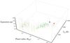 |
Fig. 1 3D plot of the known transiting exoplanets. The quantities on the axes are the planetary radius and the temperature, and their semi-major axes. The positions of HAT-P-23 b and WASP-48 b are highlighted by a blue and red point, respectively. Data taken from the TEPcat catalogue. |
1.1. HAT-P-23
The HAT-P-23 system, discovered by Bakos et al. (2011), is composed of a G0 dwarf star (mass 1.13 M⊙, radius 1.20 R⊙, and metallicity + 0.13) and a hot Jupiter (mass 2.09 MJup and radius 1.37 RJup) revolving around its parent star on a circular orbit with a period of P = 1.2 d. Using the SOPHIE spectrograph, Moutou et al. (2011) measured the projected spin-orbit angle through observation of the Rossiter-McLaughlin (R-M) effect. Their finding of λ = 15° ± 22° suggests an aligned and prograde planetary orbit. A reanalysis of the main parameters of the system was performed by Ramón-Fox & Sada (2013). Recently, O’Rourke et al. (2014) reported accurate photometry of planet occultations observed at 3.6 μm and 4.5 μm with the Spitzer space telescope and at H and KS bands with the Hale Telescope. They found the emission spectrum to be consistent with a planetary atmosphere having a low efficiency of energy transport from its day-side to night-side, no thermal inversion and a lack of strongly absorbing substances, similar to the case of WASP-19 b (Mancini et al. 2013c).
1.2. WASP-48
WASP-48 is a TEP system composed of a slightly evolved F-type star (mass 1.19 M⊙, radius 1.75 R⊙, and metallicity −0.12) and an inflated hot Jupiter (mass 0.98 MJup, radius 1.67 RJup, and an orbital period of P = 2.1 d; Enoch et al. 2011). The lithium abundance and the absence of Ca II H and K emission suggests that the host star is old and evolving off the main sequence. However, by measuring the age from the rotation period, the star seems to be much younger (Enoch et al. 2011). This discrepancy can be explained if tidal forces between the planet and the parent star have spun up the latter, making it difficult to obtain a reasonable value for the age based on gyrochronology (e.g. Pont 2009). The emission spectrum of WASP-48 b was also investigated by O’Rourke et al. (2014) through IR observations of the planet occultations with the Spitzer and the Hale telescopes. The nature of the atmosphere of WASP-48 b was found to be very similar (moderate energy recirculation, no temperature inversion, absence of strong absorbers) to that of HAT-P-23 b.
2. Observations and data reduction
Details of the observations presented in this work.
In this section we present photometric observations of eight transits of HAT-P-23 b and seven of WASP-48 b. For both systems, one transit was observed with a multi-band imaging camera. One transit of WASP-48 was simultaneously monitored with two telescopes from the same observatory. The details of the observations are summarized in Table 1.
2.1. Calar Alto 1.23 m telescope
Seven transits of HAT-P-23 b and four of WASP-48 b were remotely observed using the Zeiss 1.23 m telescope at the Calar Alto Observatory in Spain. The telescope has an equatorial mount and is equipped with a DLR-MKIII camera positioned at its Cassegrain focus. The CCD, which was used unbinned, has 4096 × 4096 pixels and a field of view (FOV) of 21.5′ × 21.5′ leading to a resolution of 0.32′′ pixel-1. The telescope was autoguided and defocussed for all science observations. This observing mode consists of using the telescope out of focus to spread the light of the stars in the FOV on many more pixels of the CCD than normal in-focus observations. In this way it is possible to use longer exposures, greatly increasing the signal-to-noise ratio (S/N) and reducing the uncertainties due to many sources of noise (Southworth et al. 2009). In our cases, the exposure times were fine-tuned at the beginning of each observation, together with the amount of defocussing, in order to properly optimize the S/N and have a maximum count per pixel for the target star between 25 000 to 35 000 ADUs. Once the defocussing amount was set, it was kept fixed for the entire monitoring of the transit (a typical PSF of the target covered a region with a diameter from 15 to 25 pixel). In some cases, it was necessary to modify the exposure time during the night to avoid the CCD saturation or to account for changes in counts caused by variation of the air mass of the target or weather conditions (e.g. dramatic variations of the external temperature or sudden appearance of cirrus and veils). The filter used to observe HAT-P-23 b was Cousins R; for WASP-48 b the first and last transits were observed through Cousins R and the other two transits through Cousins I (Table 1).
2.2. Cassini 1.52 m telescope
Two transit light curves of WASP-48 were obtained on 2011 May 23 and 25 at the Astronomical Observatory of Bologna in Loiano, Italy. Observations were carried out with BFOSC (Bologna Faint Object Spectrograph and Camera) mounted at the Cassegrain focus of the 1.52 m Cassini telescope (see Table 1). The 1300 × 1340 pixels CCD has a FOV of 13′ × 12.6′ resulting in a resolution of 0.58′′ pixel-1. For both transits a Gunn-r filter was used and the telescope was autoguided and defocussed. During the acquisition of the science images, the CCD was windowed to decrease the readout time, thus achieving a higher temporal cadence.
2.3. Calar Alto 2.2 m telescope
One transit of each object was observed with the Bonn University Simultaneous Camera (BUSCA, Reif et al. 1999) mounted on the Calar Alto 2.2 m telescope. BUSCA can obtain photometry in four different passbands simultaneously, the incoming light being split by dichroics. Each of the four channels has a 4096 × 4096 pixel CCD, which were used with 2 × 2 binning to give a plate scale of 0.35′′ pixel-1. The FOV of each channel depends on the filter in the light beam, which is 5.8′ in diameter for the Thuan-Gunn and Strömgren filters and 12′ × 12′ for the Cousins I filter. The telescope was autoguided and defocussed during both observing sequences.
Unfortunately, the BUSCA controller requires that the same exposure time be used in all four channels. The exposure times were therefore chosen to avoid saturation in the r band, for which the count rate was highest. This meant that the redder channels yielded better-quality data than the bluer channels, especially the u band.
2.4. Data reduction
Data reduction was performed using standard methods. Bias and flat-field images on the sky were collected before and during twilight, respectively, and median-combined to generate master bias and flat-field frames. These were used to calibrate the science images. Light curves were then obtained using aperture photometry algorithms from daophot (Stetson 1987) as implemented in the idl2-based defot pipeline (see Southworth et al. 2014, and references therein), which uses subroutines from the NASA astrolib3 library.
The sizes of the software apertures used for the aperture photometry are listed in Table 1, and were chosen to be those that gave the lowest out-of-transit (OOT) scatter. We noticed that changes in the aperture size of both the target region and the sky annulus do not affect the overall light-curve shape, but do cause a slight variation in the scatter of the data points. Once the aperture sizes were set, we extracted instrumental magnitudes for the target and possible comparison stars in the FOV. Pointing variations were corrected by cross-correlating each image against a reference frame. The light curves were then detrended by a second-order polynomial whilst optimising the weights of an ensemble of comparison stars. The choice of the comparison stars was carried out according to their brightness, by comparing the different OOT scatter and taking the combination that gave the lowest scatter.
3. Light curve analysis
We separately analyzed each of the light curves observed using the jktebop4 code (see Southworth 2008, and references therein). jktebop fits an observed light curve with a synthetic one, constructed according to the values of a set of initial parameters. Some of the input parameters are left free to vary until the best fit is reached. The main photometric parameters that we can measure with jktebop are the orbital inclination, i; the orbital period, P; the transit midpoint, T0; and the sum and ratio of the fractional radii of the star and planet, rA + rb and k = rb/rA. The fractional radii are defined as rA = RA/a and rb = Rb/a, where a is the orbital semi-major axis, and RA and Rb are the absolute radii of the star and the planet, respectively.
We assumed circular orbits for both the planetary systems (Enoch et al. 2011; O’Rourke et al. 2014). The values of the planet-star mass ratio were fixed to those obtained using the estimated masses from the discovery papers. The limb darkening effect on the light curves was taken into account by modelling it using a quadratic law, and we checked that the difference in the results obtained using a linear or a logarithmic law is negligible.
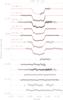 |
Fig. 2 Light curves of transits of HAT-P-23 b, observed with the Calar Alto 1.23 m telescope, compared with the best-fitting models given by jktebop. The date of each observation is given next to the corresponding light curve. The residuals from the fits are shown at the base of the figure in the same order as the light curves. |
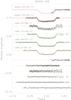 |
Fig. 3 Light curves of transits of WASP-48 b, observed with the Cassini 1.52-m (“loiano”) and Calar Alto 1.23 m (“caha”) telescopes, compared with the best-fitting curves given by jktebop. The date of each observation is given next to the corresponding light curve. The residuals from the fits are shown at the base of the figure in the same order as the light curves. |
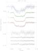 |
Fig. 4 A planetary transit event of HAT-P-23 b as observed with the BUSCA instrument mounted on the CAHA 2.2 m telescope. The light curves in the Thuan-Gunn ugrz are shown from top to bottom and are compared to the best jktebop fits. The residuals are plotted at the base of the figure. |
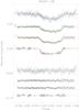 |
Fig. 5 As for Fig. 4 but for WASP-48 b. A Cousins I filter was used in the reddest arm of BUSCA, while a Strömgren u was used in the bluest arm. |
The fits of the light curves were performed using theoretical values of the limb darkening coefficients (Claret 2000, 2004a) and by fitting the linear coefficients whilst fixing the quadratic coefficients but perturbing them during the error analysis simulations. The atmospheric parameters of the stars HAT-P-23 A and WASP-48 A, assumed for deriving the initial values of the limb-darkening coefficients, and the weighted-mean values of the limb-darkening coefficient obtained from the fit of the light curves are listed in Table 2.
Stellar atmospheric parameters used to calculate the limb darkening coefficients, and weighted-mean values of the linear coefficients obtained from the fit of the light curves.
Since the aper routine, which we used to perform aperture photometry on the calibrated science images, commonly underestimates the error bars, we enlarged them for each data set by multiplying the error bar for each photometric point by the square root of the  obtained through an initial fit of the corresponding light curve. We then further inflated the errors using the β approach (e.g. Pont et al. 2006; Gillon et al. 2006; Winn et al. 2007) to take into account the presence of systematic effects and correlated noise.
Times of transit midpoint of HAT-P-23 b and their residuals.
To assign the uncertainties to each parameter obtained from the fitting process, we generated 10 000 simulations with a Monte Carlo algorithm and also used a residual-permutation algorithm (Southworth 2008). Since none of the two techniques systematically gives lower uncertainties, we took the larger of the 1σ values obtained using the two algorithms. The best-fitting model and the residuals for each of the 21 light curves are shown in Figs. 2–5.
3.1. New orbital ephemeris
We refined the orbital periods of both planets by using our new photometric data and transit timings available in the literature or at the ETD5 website.
We made a linear fit to the transit midpoints versus cycle numbers in order to improve the ephemeris. All the transits considered in the linear fit for the two planetary systems are listed in Tables 3 and 4. The new values for the ephemeris found from the fits are  (1)and
  (2)for HAT-P-23 and WASP-48, respectively. The numbers in brackets are the errors relative to the last digit, and E represents the cycle number.
If a TEP system, known to be composed of a parent star and a planet, hosts other planets, the gravitational interaction between the planetary components results in a periodic delay and advance in the times of transit of the known planet. We checked for a possible third component in the HAT-P-23 and WASP-48 systems by looking to see whether there was a periodic variation in the transit times of the known planets.
The residuals from the linear fits are plotted in Figs. 6 and 7 as a function of cycle number and do not show any clear systematic deviation from the predicted transit times. However, the quality of the fits,  for HAT-P-23 and
  for WASP-48, indicates that a linear ephemeris is not a good match to the observations in both the cases. Based on our experience with a similar situation in previous studies (e.g. Southworth et al. 2012a,b; Mancini et al. 2013a,c), we conservatively do not interpret the large
  values as a sign of transit timing variations, but as an underestimation of the uncertainties in the various T0 measurements.
3.2. Final photometric parameters
The final photometric parameters for the HAT-P-23 system were obtained taking into account only the complete transit light curves (i.e. discarding the two partial ones). This choice was made after noticing that the , relative to the ratio of the radii of the planet and the star, decreases significantly (from 4.37 to 0.99) when rejecting them. Concerning WASP-48, we discarded the incomplete light curve and those with very high scatter (i.e. the light curve observed on 2011 Aug. 23 with the CA 1.23 m and with BUSCA in the u band). Even discarding three light curves, the for the k parameter remained rather high (8.48). This discrepancy is discussed further in Sect. 4.1.
The final values were obtained as a weighted mean of all the transits taken into account. The relative errors, obtained from the weighted mean, are rescaled by multiplying them for the relative .
Times of transit midpoint of WASP-48 b and their residuals.
The parameters of the jktebop fits to each of our light curves are given in Tables 5 and 6 for HAT-P-23 and WASP-48, respectively. These tables also show the final photometric parameters in bold font, and the results from the discovery papers for comparison.
4. Physical properties of HAT-P-23 and WASP-48
Following the methodology used by Southworth (2010), the main physical parameters of the TEP systems HAT-P-23 and WASP-48 were found from the photometric parameters deduced from the parameters available in the literature (see Table 7 for values and references), and by interpolating within the tabulated predictions of five sets of theoretical stellar models (Claret 2004b; Demarque et al. 2004; Pietrinferni et al. 2004; VandenBerg et al. 2006; Dotter et al. 2008). In brief, an initial estimate of the stellar mass was specified and the observed quantities were compared to the ones predicted by stellar models for this mass. The mass was then iteratively adjusted to find the best agreement between the observed and expected values.
Since the radius versus mass relation varies according to the age of the star, the interpolation was performed for different ages of the system, starting from 0.1 Gyr until the end of the main-sequence lifetime of the star, in steps of 10 Myr. The output set of physical parameters is the one that gives the best agreement between the predicted and the measured quantities. Separate sets of results were calculated using each of the five sets of theoretical model tabulations.
The final values found are shown in Table 8 for HAT-P-23 and Table 9 for WASP-48. Most quantities have two error bars, and in these cases the first is a statistical error obtained by propagating the uncertainties on the input measurements, and the second is a systematic error which is the scatter of the results from each of the five different sets of theoretical models (see Southworth 2009).
 |
Fig. 6 Residuals of the timing of mid-transit of HAT-P-23 versus a linear ephemeris. The points indicate literature results (blue), data obtained from the TRESCA catalogue (red), and our data (green). |
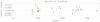 |
Fig. 7 Residuals of the timing of mid-transit of WASP-48 versus a linear ephemeris. The points indicate the value from the discovery paper (blue), data obtained from the TRESCA catalogue (red), and our data (green). |
Photometric properties of the HAT-P-23 system derived by fitting the light curves with jktebop.
Photometric properties of the WASP-48 system derived by fitting the light curves with jktebop.
4.1. Radius versus wavelength variation
Photometric observations of planetary transit events through different filters allow us to measure the apparent radius of transiting planets in each passband, obtaining an insight of the composition of their atmosphere (e.g. Southworth et al. 2012b; Copperwheat et al. 2013; Nikolov et al. 2013; Mancini et al. 2013c; Narita et al. 2013; Chen et al. 2014). We used our multi-band data to investigate possible variations of the radius of HAT-P-23 b and WASP-48 b in different optical passbands.
Spectroscopic parameters of the stars HAT-P-23 A and WASP-48 A.
Physical properties for the HAT-P-23 system.
We phased all the light curves collected with the same telescope and filter combination and, following the strategy used by Southworth et al. (2012b), we re-fitted them and the BUSCA curves with all parameters fixed to the final values listed in Tables 8 and 9, with the exception of k. This approach allows the sources of uncertainty common to all data sets to be removed, maximizing the accuracy of estimations of the planet/star radius ratio as a function of wavelength. Because of the very large uncertainty, the values of k measured in the u band were ignored. The results in the other bands are shown in Fig. 8 for HAT-P-23 b and Fig. 9 for WASP-48 b. The vertical bars represent the relative errors in the measurements and the horizontal bars show the full width at half-maximum (FWHM) transmission of the passbands used. Transmission curves of the adopted filters are shown in the bottom panel.
For illustration, the results obtained for HAT-P-23 b are compared with three spectra calculated from 1D model atmospheres by Fortney et al. (2010) for a Jupiter-mass planet with a surface gravity of gb = 25 m s-2, a base radius of 1.25 RJup at 10 bar, and Teq = 2000 K. The first model (red line) is run in an isothermal case taking into account chemical equilibrium and the presence of strong absorbers, such as TiO and VO. The second model (green line) is obtained omitting the presence of the strong absorbers. The last model (blue line) is obtained by artificially removing the strong absorbers, as in the previous case, but also increasing the H2/He Rayleigh scattering by a factor of 100. The values of k for WASP-48 b were compared with another model from Fortney et al. (2010) similar to previous ones, but for a Jupiter-mass planet with a surface gravity of gb = 10 m s-2 and without strong absorbers.
The precision of the final results does not allow us to discriminate among the models. We can only note that, since there are no large variations in the planet’s radius at shorter wavelengths within the experimental uncertainties, the atmospheres of the two planets should be quite transparent and not affected by large Rayleigh scattering. They are well suited to further investigation at the optical wavelengths with more precise instruments.
Final results for the physical parameters of WASP-48 obtained in this work compared to those of the discovery paper.
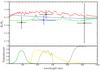 |
Fig. 8 Variation of the planetary radius of HAT-P-23 b, in terms of planet/star radius ratio, with wavelength. The black points are from the transit observed with BUSCA, while the blue point is the weighted-mean results coming from the seven transits observed in Cousins R with the CA 1.23 m telescope. The vertical bars represent the errors in the measurements and the horizontal bars show the FWHM transmission of the passbands used. The observational points are compared with three synthetic spectra for a Jupiter planet with a surface gravity of gb = 25 m s-2 and Teq = 2000 K. The synthetic spectra in green and blue do not include TiO and VO opacity, while the spectrum in red does, based on equilibrium chemistry. With respect to the model identified with the green line, the blue one has H2/He Rayleigh scattering increased by a factor of 100. An offset is applied to all three models to provide the best fit to our radius measurements. Transmission curves of the filters used are shown in the bottom panel. |
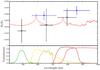 |
Fig. 9 Variation of the planetary radius of WASP-48 b, in terms of planet/star radius ratio, with wavelength. The black points are from the transit observed with BUSCA, while the blue points are the weighted-mean results coming from the two transits observed in Cousins R and the two in I with the CA 1.23 m telescope. The vertical bars represent the errors in the measurements and the horizontal bars show the FWHM transmission of the passbands used. The observational points are compared with a synthetic spectrum for a Jupiter planet with a surface gravity of gb = 10 m s-2 and Teq = 2000 K, which does not include TiO and VO opacity. An offset is applied to all three models to provide the best fit to our radius measurements. Transmission curves of the filters used are shown in the bottom panel. |
4.2. Eclipsing binary
The eclipsing binary candidate NSVS 3071474 is located at sky position RA(J2000) = 19 24 03.821 and Dec(J2000) = 55 27 33.33. It is sufficiently close to WASP-48 that it is present in the FOV of some of the transits that we monitored. We have extracted light curves of this object and confirm the nature of the system to be that of a contact eclipsing binary.
We also obtained the light curve observed by the SuperWASP survey (Pollacco et al. 2006), where it is called 1SWASP J192403.81+552734.5. The phased and binned WASP data, and the light curves obtained from our frames are shown in Figs. 10 and 11, respectively.
By fitting both the WASP data, and our light curves with jktebop we obtained a measurement of the period of the eclipsing binary of 0.458998509 ± 0.000000011 days.
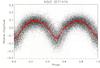 |
Fig. 10 Light curves of NSVS 3071474 (1SWASP J192403.81+ 552734.5) phased (black dots) and binned (red dots) observed by the WASP survey between 2008 and 2010. |
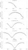 |
Fig. 11 Light curves of NSVS 3071474, the eclipsing binary close to WASP-48. The curves in the top two panels were observed with the 1.52 m Cassini telescope while the bottom two were observed with the 1.23 m Calar Alto telescope. |
5. Discussion and conclusions
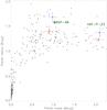 |
Fig. 12 Mass versus radius diagram of the transiting planets. The blue and red dots represent the values for HAT-P-23 and WASP-48 found in literature and obtained in this work, respectively. |
In this paper we presented refined parameters for the two TEP systems HAT-P-23 and WASP-48 obtained from new photometric data of transit events. We also presented simultaneous observations in different optical bands. Our principal results are as follows.
-
We confirmed the mass value ofHAT-P-23 b, but obtained a radius for it that is smaller by roughly 1.5 σ . This TEP now occupies a more populated region of the mass-radius diagram and is no longerfound to be one of the highly inflated transiting planets (see Fig. 12). The mean density is therefore higher than what was found in the discovery paper.
-
We obtained improved estimates of the mass and radius of both the star and the planet of the WASP-48 planetary system. The values for the stellar and planetary radius are smaller than those found in the discovery paper by roughly 2.2 σ and 2.4 σ , respectively. The masses are consistent with previous results.
-
A study of the planet’s radius variation as a function of optical wavelength, based on the data presented in this work, do not indicate any large variation for either planet, suggesting that their atmospheres are not affected by a large Rayleigh scattering. Further investigations of the transmission spectra of these two planets are needed to validate this statement.
-
Finally, we also presented new light curves for the eclipsing binary NSVS 3071474, refining the measurement of the orbital period to be 0.458998509 (11) days.
TEPcat is the catalogue of the physical properties of transiting planetary systems (Southworth 2011) and is available at http://www.astro.keele.ac.uk/jkt/tepcat/
The acronym idl stands for Interactive Data Language and is a trademark of ITT Visual Information Solutions. For further details see: http://www.ittvis.com/ProductServices/IDL.aspx
The astrolib subroutine library is distributed by NASA. For further details see: http://idlastro.gsfc.nasa.gov/
The source code of jktebop is available at http:// www.astro.keele.ac.uk/jkt/codes/jktebop.html
The Exoplanet Transit Database (ETD) website can be found at http://var2.astro.cz/ETD
Acknowledgments
Based on observations obtained with the 1.52 m Cassini telescope at the OAB Observatory in Loiano (Italy), and with the 1.23 m and 2.2 m telescopes at the Centro Astronómico Hispano Alemán (CAHA) at Calar Alto (Spain), jointly operated by the Max-Planck Institut für Astronomie and the Instituto de Astrofísica de Andalucía (CSIC). The reduced light curves presented in this work will be made available at the CDS (http://cdsweb.u-strasbg.fr/). Special thanks go to D. Pollacco and A. Cameron for allowing us to use both the public and the unpublished WASP data of the eclipsing binary NSVS 3071474. S.C. thanks M. Line, J. Fortney and his group for useful discussions and for the kind hospitality at UCSC. We acknowledge the use of the following internet-based resources: the ESO Digitized Sky Survey; the TEPCat catalog; the SIMBAD data base operated at CDS, Strasbourg, France; and the arXiv scientific paper preprint service operated by Cornell University.
References
- Anderson, D. R., Smith, A. M. S., Lanotte, A. A., et al. 2010, MNRAS, 416, 2108 [Google Scholar]
- Bakos, G., Hartman, J., Torres, G., et al. 2011, ApJ, 742, 116 [NASA ADS] [CrossRef] [Google Scholar]
- Baraffe, I., Chabrier, G., Fortney, J., & Sotin, C. 2014, Protostar and Planet VI Conf. Proc., 763 [Google Scholar]
- Brown, T. M. 2001, ApJ, 553, 1006 [NASA ADS] [CrossRef] [Google Scholar]
- Ciceri, S., Mancini, L., Southworth, J., et al. 2013, A&A, 557, A30 [NASA ADS] [CrossRef] [EDP Sciences] [Google Scholar]
- Claret, A. 2000, A&A, 363, 1081 [NASA ADS] [Google Scholar]
- Claret, A. 2004a, A&A, 428, 1001 [NASA ADS] [CrossRef] [EDP Sciences] [Google Scholar]
- Claret, A. 2004b, A&A, 424, 919 [NASA ADS] [CrossRef] [EDP Sciences] [Google Scholar]
- Chen, G., van Boekel, R., Wang, H., et al. 2014, A&A, 563, A40 [NASA ADS] [CrossRef] [EDP Sciences] [Google Scholar]
- Copperwheat, C. M., Wheatley, P. J., Southworth, J., et al. 2013, MNRAS, 434, 661 [NASA ADS] [CrossRef] [Google Scholar]
- Demarque, P., Woo, J.-H., Kim, Y.-C., & Yi, S. K. 2004, ApJS, 155, 667 [NASA ADS] [CrossRef] [Google Scholar]
- Dotter, A., Chaboyer, B., Jevremović, D., et al. 2008, ApJS, 178, 89 [NASA ADS] [CrossRef] [Google Scholar]
- Enoch, B., Anderson, D. R., Barros, S. C. C., et al. 2011, ApJ, 142, 86 [Google Scholar]
- Fortney, J. J., Shabram, M., Showman, A. P., et al. 2010, ApJ, 709, 1396 [NASA ADS] [CrossRef] [Google Scholar]
- Gillon, M., Pont, F., Moutou, C., et al. 2006, A&A, 459, 249 [NASA ADS] [CrossRef] [EDP Sciences] [Google Scholar]
- Ginzburg, S., & Sari, R. 2015, ApJ, 803, 111 [NASA ADS] [CrossRef] [Google Scholar]
- Mancini, L., Southworth, J., Ciceri, S., et al. 2013a, A&A, 551, A11 [NASA ADS] [CrossRef] [EDP Sciences] [Google Scholar]
- Mancini, L., Nikolov, N., Southworth, J., et al. 2013b, MNRAS, 430, 2932 [NASA ADS] [CrossRef] [Google Scholar]
- Mancini, L., Ciceri, S., Chen, G., et al. 2013c, MNRAS, 436, 2 [NASA ADS] [CrossRef] [Google Scholar]
- Mancini, L., Southworth, J., Ciceri, S., et al. 2014a, A&A, 562, A126 [NASA ADS] [CrossRef] [EDP Sciences] [Google Scholar]
- Mancini, L., Southworth, J., Ciceri, S., et al. 2014b, MNRAS, 443, 2391 [NASA ADS] [CrossRef] [Google Scholar]
- Mancini, L., Southworth, J., Ciceri, S., et al. 2014c, A&A, 568, A127 [NASA ADS] [CrossRef] [EDP Sciences] [Google Scholar]
- Moutou, C., Díaz, R. F., Udry, S., & Hébrard, G. 2011, A&A, 533, A113 [NASA ADS] [CrossRef] [EDP Sciences] [Google Scholar]
- Narita, N., Fukui, A., Ikoma, M., et al. 2013, ApJ, 773, 144 [NASA ADS] [CrossRef] [Google Scholar]
- Nikolov, N., Chen, G., Fortney, J. J., et al. 2013, A&A, 533, A26 [NASA ADS] [CrossRef] [EDP Sciences] [Google Scholar]
- O’Rourke, J. G., Knutson, H. A., Zhao, M., et al. 2014, ApJ, 781, 109 [NASA ADS] [CrossRef] [Google Scholar]
- Pietrinferni, A., Cassisi, S., Salaris, M., & Castelli, F. 2004, ApJ, 612, 168 [NASA ADS] [CrossRef] [Google Scholar]
- Pollacco, D. L., Skillen, I., Collier Cameron, A., et al. 2006, PASP, 118, 1407 [NASA ADS] [CrossRef] [Google Scholar]
- Pont, F. 2009, MNRAS, 396, 1789 [NASA ADS] [CrossRef] [Google Scholar]
- Pont, F., Zucker, S., & Queloz, D. 2006, MNRAS, 373, 231 [NASA ADS] [CrossRef] [Google Scholar]
- Ramón-Fox, F. G., & Sada, P. V. 2013, Rev. Mex. Astron. Astrofís., 49, 71 [NASA ADS] [Google Scholar]
- Reif, K., Bagschik, K., de Boer, K. S., et al. 1999, Proc. SPIE, 3649, 109 [Google Scholar]
- Seager, S., & Mallén-Ornelas, G. 2003, ApJ, 585, 1038 [NASA ADS] [CrossRef] [Google Scholar]
- Seager, S., & Sasselov, D. D. 2000, ApJ, 537, 916 [NASA ADS] [CrossRef] [Google Scholar]
- Seeliger, M., Dimitrov, D., Kjurkchieva, D., et al. 2014, MNRAS, 441, 304 [NASA ADS] [CrossRef] [Google Scholar]
- Southworth, J. 2008, MNRAS, 386, 1644 [NASA ADS] [CrossRef] [Google Scholar]
- Southworth, J. 2009, MNRAS, 394, 272 [NASA ADS] [CrossRef] [Google Scholar]
- Southworth, J. 2010, MNRAS, 408, 1689 [NASA ADS] [CrossRef] [Google Scholar]
- Southworth, J. 2011, MNRAS, 417, 2166 [NASA ADS] [CrossRef] [Google Scholar]
- Southworth, J., Wheatley, P. J., & Sams, G. 2007, MNRAS, 379, L11 [NASA ADS] [CrossRef] [Google Scholar]
- Southworth, J., Hinse, T. C., Jørgensen, U. G., et al. 2009, MNRAS, 396, 1023 [NASA ADS] [CrossRef] [Google Scholar]
- Southworth, J., Dominik, M., Jørgensen, U. G., et al. 2011, A&A, 527, A8 [NASA ADS] [CrossRef] [EDP Sciences] [Google Scholar]
- Southworth, J., Bruni, I., Mancini, L., & Gregorio, J. 2012a, MNRAS, 420, 2580 [NASA ADS] [CrossRef] [Google Scholar]
- Southworth, J., Mancini, L., Maxted, P. F. L., et al. 2012b, MNRAS, 422, 3099 [NASA ADS] [CrossRef] [Google Scholar]
- Southworth, J., Hinse, T. C., Burgdorfet, M., et al. 2014, MNRAS, 444, 776 [NASA ADS] [CrossRef] [Google Scholar]
- Sozzetti, A., Torres, G., Charbonneau, D., et al. 2007, ApJ, 664, 1190 [NASA ADS] [CrossRef] [Google Scholar]
- Sozzetti, A., Bonomo, A. S., Biazzo, K., et al. 2015, A&A, 575, L15 [NASA ADS] [CrossRef] [EDP Sciences] [Google Scholar]
- Spiegel, D. S., & Burrows, A. 2013, ApJ, 772, 76 [NASA ADS] [CrossRef] [Google Scholar]
- Stetson, P. B. 1987, PASP, 99, 191 [NASA ADS] [CrossRef] [Google Scholar]
- Torres, G., Winn, J. N., & Holman, M. W. 2008, ApJ, 677, 1324 [NASA ADS] [CrossRef] [Google Scholar]
- Torres, G., Fischer, D. A., Sozzetti, A., et al. 2012, ApJ, 757, 161 [NASA ADS] [CrossRef] [Google Scholar]
- VandenBerg, D. A., Bergbusch, P. A., & Dowler, P. D. 2006, ApJS, 162, 375 [NASA ADS] [CrossRef] [MathSciNet] [Google Scholar]
- Winn, J. N., Holman, M. J., Bakos, G. Á., et al. 2007, AJ, 134, 1707 [NASA ADS] [CrossRef] [Google Scholar]
All Tables
Stellar atmospheric parameters used to calculate the limb darkening coefficients, and weighted-mean values of the linear coefficients obtained from the fit of the light curves.
Photometric properties of the HAT-P-23 system derived by fitting the light curves with jktebop.
Photometric properties of the WASP-48 system derived by fitting the light curves with jktebop.
Final results for the physical parameters of WASP-48 obtained in this work compared to those of the discovery paper.
All Figures
|
Fig. 1 3D plot of the known transiting exoplanets. The quantities on the axes are the planetary radius and the temperature, and their semi-major axes. The positions of HAT-P-23 b and WASP-48 b are highlighted by a blue and red point, respectively. Data taken from the TEPcat catalogue. |
| In the text | |
|
Fig. 2 Light curves of transits of HAT-P-23 b, observed with the Calar Alto 1.23 m telescope, compared with the best-fitting models given by jktebop. The date of each observation is given next to the corresponding light curve. The residuals from the fits are shown at the base of the figure in the same order as the light curves. |
| In the text | |
|
Fig. 3 Light curves of transits of WASP-48 b, observed with the Cassini 1.52-m (“loiano”) and Calar Alto 1.23 m (“caha”) telescopes, compared with the best-fitting curves given by jktebop. The date of each observation is given next to the corresponding light curve. The residuals from the fits are shown at the base of the figure in the same order as the light curves. |
| In the text | |
|
Fig. 4 A planetary transit event of HAT-P-23 b as observed with the BUSCA instrument mounted on the CAHA 2.2 m telescope. The light curves in the Thuan-Gunn ugrz are shown from top to bottom and are compared to the best jktebop fits. The residuals are plotted at the base of the figure. |
| In the text | |
|
Fig. 5 As for Fig. 4 but for WASP-48 b. A Cousins I filter was used in the reddest arm of BUSCA, while a Strömgren u was used in the bluest arm. |
| In the text | |
|
Fig. 6 Residuals of the timing of mid-transit of HAT-P-23 versus a linear ephemeris. The points indicate literature results (blue), data obtained from the TRESCA catalogue (red), and our data (green). |
| In the text | |
|
Fig. 7 Residuals of the timing of mid-transit of WASP-48 versus a linear ephemeris. The points indicate the value from the discovery paper (blue), data obtained from the TRESCA catalogue (red), and our data (green). |
| In the text | |
|
Fig. 8 Variation of the planetary radius of HAT-P-23 b, in terms of planet/star radius ratio, with wavelength. The black points are from the transit observed with BUSCA, while the blue point is the weighted-mean results coming from the seven transits observed in Cousins R with the CA 1.23 m telescope. The vertical bars represent the errors in the measurements and the horizontal bars show the FWHM transmission of the passbands used. The observational points are compared with three synthetic spectra for a Jupiter planet with a surface gravity of gb = 25 m s-2 and Teq = 2000 K. The synthetic spectra in green and blue do not include TiO and VO opacity, while the spectrum in red does, based on equilibrium chemistry. With respect to the model identified with the green line, the blue one has H2/He Rayleigh scattering increased by a factor of 100. An offset is applied to all three models to provide the best fit to our radius measurements. Transmission curves of the filters used are shown in the bottom panel. |
| In the text | |
|
Fig. 9 Variation of the planetary radius of WASP-48 b, in terms of planet/star radius ratio, with wavelength. The black points are from the transit observed with BUSCA, while the blue points are the weighted-mean results coming from the two transits observed in Cousins R and the two in I with the CA 1.23 m telescope. The vertical bars represent the errors in the measurements and the horizontal bars show the FWHM transmission of the passbands used. The observational points are compared with a synthetic spectrum for a Jupiter planet with a surface gravity of gb = 10 m s-2 and Teq = 2000 K, which does not include TiO and VO opacity. An offset is applied to all three models to provide the best fit to our radius measurements. Transmission curves of the filters used are shown in the bottom panel. |
| In the text | |
|
Fig. 10 Light curves of NSVS 3071474 (1SWASP J192403.81+ 552734.5) phased (black dots) and binned (red dots) observed by the WASP survey between 2008 and 2010. |
| In the text | |
|
Fig. 11 Light curves of NSVS 3071474, the eclipsing binary close to WASP-48. The curves in the top two panels were observed with the 1.52 m Cassini telescope while the bottom two were observed with the 1.23 m Calar Alto telescope. |
| In the text | |
|
Fig. 12 Mass versus radius diagram of the transiting planets. The blue and red dots represent the values for HAT-P-23 and WASP-48 found in literature and obtained in this work, respectively. |
| In the text | |
Current usage metrics show cumulative count of Article Views (full-text article views including HTML views, PDF and ePub downloads, according to the available data) and Abstracts Views on Vision4Press platform.
Data correspond to usage on the plateform after 2015. The current usage metrics is available 48-96 hours after online publication and is updated daily on week days.
Initial download of the metrics may take a while.