| Issue |
A&A
Volume 585, January 2016
|
|
|---|---|---|
| Article Number | A38 | |
| Number of page(s) | 8 | |
| Section | Interstellar and circumstellar matter | |
| DOI | https://doi.org/10.1051/0004-6361/201425112 | |
| Published online | 15 December 2015 | |
Allsky NICER and NICEST extinction maps based on the 2MASS near-infrared survey⋆
1
Department of Physics, PO Box 64, 00014 University of Helsinki,
Finland
e-mail:
This email address is being protected from spambots. You need JavaScript enabled to view it.
2
Institut UTINAM, CNRS UMR 6213, OSU THETA, Université de
Franche-Comté, 41 bis avenue de l’Observatoire, 25000
Besançon,
France
Received: 5 October 2014
Accepted: 22 October 2015
Abstract
Context. Extinction remains one of the most reliable methods of measuring column density of nearby Galactic interstellar clouds. The current and ongoing near-infrared surveys enable the mapping of extinction over large sky areas.
Aims. We produce allsky extinction maps using the 2MASS near-infrared survey.
Methods. We use the NICER and NICEST methods to convert the near-infrared colour excesses to extinction estimates. The results are presented in Healpix format at the resolutions of 3.0, 4.5, and 12.0 arcmin.
Results. The main results of this study are the calculated J-band extinction maps. The comparison with earlier large-scale extinction mappings shows good correspondence but also demonstrates the presence of resolution-dependent bias. A large fraction of the bias can be corrected by using the NICEST method.
Conclusions. For individual regions, best extinction estimates are obtained by careful analysis of the local stellar population and the use of the highest resolution afforded by the stellar density. However, the uniform allsky maps should still be useful for many global studies and as the first step into the investigation of individual clouds.
Key words: ISM: clouds / infrared: ISM / submillimeter: ISM / dust, extinction / stars: formation
Final extinction maps are only available at the CDS via anonymous ftp to cdsarc.u-strasbg.fr (130.79.128.5) or via http://cdsarc.u-strasbg.fr/viz-bin/qcat?J/A+A/585/A38
© ESO, 2015
1. Introduction
Extinction measurements are one of the main methods by which the column density of interstellar clouds can be measured. With the development of near-infrared (NIR) observations, it has become possible to extend the studies into dense clouds. The usual range accessed by NIR observations is 1–20 mag of visual extinction, AV. However, with dedicated deep observations, even higher values can be measured. This also makes NIR studies relevant for studies of star formation from the formation of molecular clouds to the structure of individual dense cores.
In the optical regime, extinction has been mapped using the star-counting method (see, e.g. Dobashi et al. 2005). The same technique can be extended to NIR wavelengths, but it is more common to use the colour excesses of individual stars (e.g. Cambresy et al. 1997, and references below). This is based on two observations. First, the dispersion of the intrinsic colours of the stars is relatively small at NIR wavelengths (e.g. Lombardi & Alves 2001; Cambrésy et al. 2002; Davenport et al. 2014). Secondly, the variations of the NIR extinction curve are also small (e.g. Cardelli et al. 1989; Wang & Jiang 2014). Thus, the comparison of the observed NIR colours and the expected intrinsic colour gives a good estimate of the extinction. To bring the uncertainty down to a few tenths of visual magnitude, the data need to average over ten or more stars. Furthermore, to take into account the variations of stellar colours over the sky, the intrinsic colour is estimated using a nearby extinction-free area. Although each star gives an AV estimate for a very narrow line of sight (LOS), the final resolution is determined by the stellar density. With the 2MASS survey (Skrutskie et al. 2006), a resolution of ~1 arcmin can be reached but this degrades rapidly towards high Galactic latitudes.
The extinction of several large areas has already been mapped using the 2MASS survey. These include the Polaris Flare (Cambrésy et al. 2001), the Pipe nebula (Lombardi et al. 2006), Ophiuchus and Lupus (Lombardi et al. 2008), Taurus (Padoan et al. 2002; Lombardi et al. 2010), Orion (Lombardi et al. 2011, 2014), and Corona Australis (Alves et al. 2014). Most studies have used the optimised multifrequency methods the near-infrared color excess revised (NICER; Lombardi & Alves 2001) or NICEST (Lombardi 2009) to combine the information of the J − H and H − K colours. Depending on the region and its local density of background stars, the spatial resolution of these maps varies from one arcmin to a few arcmin. In Cambrésy et al. (2002), instead of using a fixed spatial resolution, the resolution was varied based on the local stellar density, thus keeping the signal-to-noise ratio (S/N) approximately constant.
The first all-sky maps of NIR extinction were presented by Rowles et al. (2009) and Dobashi (2011), the latter including an extensive catalogue of dark clouds detected in extinction. Dobashi et al. (2013) included a further modification where the Besançon model of the Galactic stellar populations was used to correct estimates of stellar intrinsic colours. These papers included extinction maps based on the J − H and H − K colours separately, but no all-sky NICER and NICEST maps have been published so far.
In this paper we describe the calculation of all-sky NIR extinction maps with the NICER and NICEST methods. The structure of the paper is the following. In Sect. 2 we describe the methods, including the calculation of the intrinsic stellar colours. In Sect. 3 we describe the pre-filtering of 2MASS catalogue data. The results and comparison with some previously presented extinction maps are given in Sect. 4 before a short discussion of the findings in Sect. 5. The final conclusions are listed in Sect. 6.
2. Methods
We use two methods, NICER (Lombardi & Alves 2001) and NICEST (Lombardi 2009), to calculate J-band extinctions based on 2MASS data. Both methods are based on the comparison between the observed NIR colours and the reference colours that would correspond to zero extinction. We use the reference colours defined in Sect.3.2. Any additional extinction of intervening dust reddens the observed colours, in our case the J − H and H − K colours. In the (J − H, H − K) plane the change is determined by the amount of extinction and the shape of the extinction curve. Because of the dispersion in intrinsic stellar colours, both methods require the averaging of the extinction estimates of many individual stars.
NICER technique seeks to combine two (or more) colour measurements in an optimal way. It is a generalisation of the earlier Near-Infrared Colour Excess (NICE) method that deals with single NIR colours (Lada et al. 1994). In NICER the reference colours are described by their average values, ⟨ J − H ⟩ and ⟨ H − K ⟩, and their covariance matrix. The dispersion of the values should be dominated by the scatter of the intrinsic colours, not by the photometric errors of individual stars. The method first calculates extinction estimates for each star. It solves the least squares problem taking into account both the dispersion of the reference colours and the uncertainty of the colour measurements of the individual stars. In practice, the distribution of intrinsic colours must be assumed to be well characterised using just a covariance matrix and, furthermore, that the same extinction law is applicable to all stars. Once the estimates of individual stars are known, the final extinction values are obtained as spatial averages calculated with a Gaussian smoothing kernel. Because of the scatter of the intrinsic colours, there should be at least ~10 stars within the area covered by the kernel. In addition to weighted averaging, the NICER method includes the so-called sigma-clipping procedure: individual stars are not included in the average if their extinction estimates deviate more than kσσA from the average. Here kσ is a sigma-clipping threshold and σA the standard deviation of the extinction estimates of individual stars. The procedure is repeated until no more stars get eliminated. This is useful, for example, to reduce the contamination by foreground stars. For details of the implementation, see Lombardi & Alves (2001).
In the presence of column density variations, the estimates of NICE and NICER are biased. If the extinction varies within the smoothing kernel, more stars are seen through the lower extinction parts and, therefore, the average extinction is underestimated. The problem can be significant at high column densities, if column density variations are large. This applies equally in the case of steep large-scale gradients and in the case of complex structures not resolved by the chosen smoothing kernel. The NICEST method adds a correction for the bias (Lombardi 2009). This involves adjusting the weights of individual stars so that stars with higher extinction estimates have larger influence. Furthermore, a correction that depends on the slope of the cumulative star counts and on the uncertainties in the extinction of individual stars is applied to the final extinction estimate. This ensures that the result remains unbiased even when the averages are calculated using only a few stars. However, the bias correction is more efficient if averages are calculated over more stars. NICEST cannot solve the problem of such column density peaks where no background stars are observed.
In our implementations of NICER and NICEST we follow closely the descriptions given in Lombardi & Alves (2001) and Lombardi (2009). In practice, calculations are performed using Healpix pixelisation, smoothing kernels with FWHM equal to 3.0, 4.5, and 12.0 arcmin, and the reference colours described in Sects. 3.2−3.3. NICEST also requires an estimate of the slope α of the stellar density vs. magnitude, ρ ~ 10α × m. We use a single value of 0.31 (H-band) (see also Lombardi 2009; Dobashi et al. 2013). When calculated directly from the 2MASS catalogue, α shows a latitude dependence, rising from ~0.1 at Galactic poles up to ~0.34 in the plane (median values over constant latitudes). However, the value α = 0.31 is valid to within ±0.05 units for all latitudes up to | b | ~ 30°. This covers most regions where the NICEST method could be useful. We assume the parameterised extinction curve of Cardelli et al. (1989) (RV = 3.1) with AJ/E(J − H) = 2.77 and AJ/E(H − K) = 4.44. These values are not sensitive to assumptions of the selective extinction RV. For RV = 3.1 our AJ values can be converted to AV by multiplying them with 3.55.
In addition to the normal sigma-clipping procedure, we will calculate a few variations of the NICER maps, using stars selected based on their extinctions relative to other stars within the smoothing kernel. Maps Q1-Q4 correspond to different quartiles. Thus Q1 is calculated with 25% of stars with the smallest AJ values and Q4 with 25% of the largest AJ values. Finally, Q12 and Q34 employ stars below and above the median value, respectively.
Large differences are not expected between the new NICER maps and those presented in Dobashi (2011) and Dobashi et al. (2013). Those earlier maps were also based on the J − H and H − K colours of 2MASS stars, the AV values being calculated with the NICE method (Lada et al. 1994). However, with the NICER method the reliability of the extinction estimates is improved by the optimal combination of the J − H and H − K colours, the expected gain being a factor of two in the variance of the extinction estimates (Lombardi 2009). All stars detected in at least two bands are used. Compared to NICE and NICER estimates, NICEST maps should differ because of their smaller bias (and somewhat larger noise). This may be important in dense clouds because, due to the large size of the smoothing kernel, averages are calculated over a wide range of column densities. Without bias correction, the extinction values can be underestimated by tens of per cent or even more (Lombardi 2009; Juvela et al. 2015).
3. Input data
3.1. 2MASS stars
The input data consists of the 2003 data release of the 2MASS point source catalogue (PSC) (Skrutskie et al. 2006). We started by rearranging the data into files, one for each of the pixels of the Healpix NSIDE = 16 pixelisation (see Górski et al. 2005). This results in 3072 files where each file includes all the point sources falling within the corresponding healpix pixel (some 3.7 degree in size) or outside the pixel but closer than ~20.0′ of its boundaries. This allows each input file to be used independently to calculate an extinction map for an area corresponding to one healpix NSIDE = 16 pixel. When spatial smoothing is done with a Gaussian beams with FWHM = 12′ and kernel is placed at the boundary of a NSIDE = 16 pixel, the data still cover an area with more than 99.995% of the convolution kernel.
In the file conversion, we carry over the coordinates, magnitude, magnitude errors, and the flags ph_qual, rd_flag, and mp_flg. We drop all sources with mp_flg set (sources associated with known solar system objects) and further require rd_flag equal to 1, 2, or 3 and ph_qual equal to A, B, or C (best quality detections with reliable photometry). However, we do not drop sources where only one band, either J or K, fails the above selection. This was done under the assumption that the other colour (J − H or H − K) still carries useful information and the influence of the more uncertain magnitude measurement is weighted down by ensuring it has a very large error estimates. We also reject extended sources with either of the flags ext_key or gal_contam set. After these criteria we are left with a total of 409 million sources, some 87% of the full PSC catalogue.
3.2. The reference colours
In addition to the apparent magnitudes of stars behind a column of dust, extinction estimation requires information of the average intrinsic stellar colours and their covariances. For individual clouds, these are often calculated using the stars in a nearby low-extinction region. This corresponds to an idealised scenario where a foreground cloud is seen against a constant background. In this case, even if the chosen reference region is not completely free of extinction, the extinction relative to the reference region would be correctly traced. When the reference region contains significant amounts of extinction, the estimated intrinsic colours become redder and also our estimate of the dispersion of the intrinsic colours is likely to increase. Nevertheless, if the background is constant, a nearby reference region provides a good approximation of the average colour of the stars as their radiation reaches the foreground cloud. In a general case the concept of a “background star” is not well defined and depends on what part of the medium along the LOS is being studied.
For an all-sky map the procedure is even less straightforward. We need reference colours that are a compromise between the actual intrinsic stellar colours and the apparent stellar colours for the radiation reaching nearby clouds. The difference is relevant mostly at low Galactic latitudes. The reference colours should also be continuous over the whole sky to avoid discontinuities in the extinction maps. We have examined colours extracted directly from the 2MASS data and colours obtained from stars simulated with the Besançon model. Figure 1 shows six versions of the maps of J − H and H − K colours.
 |
Fig. 1 Six versions of all-sky maps of the average J − H (left frames) and H − K (right frames) colours. The first three are based on observed 2MASS sources (frames a)−c)) and the last three (frames d), f)) on stars simulated with the Besançon model. See text for details. The labels M1, M2a, and M2b refer to extinction maps where the corresponding data are used as reference colours. |
In the first maps (frame a), the values are calculated as direct averages of all stars falling inside a given NSIDE = 256 Healpix pixel (pixel size ~13.7′). These values are affected by whatever foreground extinction the stars have and, especially in the plane, the colours are strongly reddened. These are thus not a particularly good reference for extinction calculations, with the possible exception of compact clumps whose extinction is estimated relative to the local extended background. Nevertheless, we will use the average values at high-latitudes | b | > 60° as the most basic reference to be used in extinction calculations.
The second maps (frame b) is calculated also on NSIDE = 256 resolution, in each pixel dropping 30% of the stars located in the highest extinction areas. For this procedure, the extinction values were read from a NICER extinction map produced with the high-latitude reference colours (see above); only relative extinctions at scales much below one degree are needed. The 30% cut-off is arbitrary but is used to mask regions that are strongly affected by extinction (mainly by distinct nearby clouds). The results depend only weakly on the exact value of this threshold. The colours of the remaining stars are further corrected using the E(B − V) map of Schlegel et al. (1998), assuming an extinction curve with RV = 3.1. In the correction all extinction is assumed to reside between the stars and us. This results in over-correction, especially near the plane. The plots of the resulting J − H and H − K colours are included in Fig. 1b only for reference and they are not used in actual extinction calculations.
The third maps are calculated at NSIDE = 64 resolution, dropping all stars with extinction exceeding 1 mag in Fig. 1a. This means that for many pixels near the Galactic plane, no estimates can be derived. For the remaining stars below 1 mag, we apply now a small correction that is again derived from Schlegel et al. (1998)E(B − V) map, this time assuming that half of the extinction resides between the stars and us. The J − H and H − K maps are shown in Fig. 1c, where we have masked all pixels | b | < 8°. As in the frame b, the correction has removed most of the column density related structures at higher latitudes. Again, these maps are included only for illustration and are not used any further.
The last three pairs of maps in Fig. 1 are based on stars simulated using the Besançon model (Robin et al. 2014). In frames d and e we have used only stars within a distance of either 2.0 kpc or 8.0 kpc, respectively. At high latitudes, these are identical and close to the values derived from 2MASS stars. On the other hand, both J − H and H − K now decrease towards the centre of the Galactic plane. When the sample is extended to 8 kpc distances, stars in the central bulge increase J − H and H − K towards the Galactic centre. In these plots stars are not affected by any extinction. Because the extinction maps will be used mostly to examine nearby structures, it would seem necessary to assume that very distant stars are affected by at least some diffuse extinction. Thus, the light from the stars behind a nearby cloud should already be reddened when it reaches our cloud. The selected procedure is described in Sect. 3.3
3.3. Selected reference colours
Besançon model provides description of the intrinsic colours of stars as a function of Galactic location. When we examine a given region on the sky, it is likely to contain structures at different distances. Conversely, if we are examining a nearby cloud, the “background stars” can be at very different distances and they may be affected by varying amounts of extinction not related to our cloud. If we define the colour of background stars based on the radiation reaching a nearby cloud, extinction further along the LOS changes the reference colours and their dispersion. This affects the error estimates of extinction and also directly the results of the NICEST method.
The problem cannot be fully addressed without information about the distribution of interstellar medium along the LOS. If we relied directly on the intrinsic colours of Besançon stars, in the plane the values would be affected by distant stars that in reality are never observed. We attempt to make a crude correction using the following procedure. In the mid-plane we assume a diffuse extinction of AV = 1.0 mag kpc-1. This is lower than the canonical value of ~1.8 mag kpc-1 which includes the contribution of dense clouds. To estimate the dependence on Galactic height, we first examined the all-sky E(B − V) map of (Planck Collaboration XI 2014), which traces the total amount of material along the LOS. We calculated the average profile of this total extinction as a function of Galactic height, using median values calculated over all Galactic longitudes. Assuming that the profile is mostly determined by relatively nearby regions, we modelled the Galactic plane as a slab with single profile f(z) as a function of Galactic height z. When f is assumed to be an exponential function, we obtain a scale height of ~210 pc. Thus, this 3D density distribution reproduces the latitude dependence of LOS extinction as seen in the Planck E(B − V) map. The scale height is higher than the typical values quoted for the ISM. This is possibly an effect of nearby cloud complexes (Taurus-Auriga, Orion, etc.) that should not be counted in our model of diffuse extinction. Therefore, we finally adopted a steeper exponential function with a scale height 150 pc. As mentioned above, the absolute scaling is determined by using at z = 0 pc a value of 1.0 mag kpc-1.
In Fig. 1, the last frame f shows the colours that are calculated using Besançon model, including the diffuse extinction as defined above. Based on its distance and Galactic latitude, the NIR magnitudes of each star are increased with the corresponding amount, using RV = 3.1 extinction curve to calculate the NIR extinction. Stars falling beyond detection limits of 15.8, 15.1, and 14.3 mag in J, H, and K bands, respectively, are dropped. In the plane, the J − H and H − K colours are now higher because of the diffuse extinction. This should be a better reference when estimating the extinction of nearby clouds. However, we again emphasise that without a full 3D image of the interstellar medium, it is not possible to calculate the “correct” reference colours that would result in correct extinction estimates in absolute terms. The final extinction maps should not be used, for example, to estimate the distribution of interstellar medium as a function of latitude. In the plane the zero point of the extinction scale is essentially arbitrary.
In the following, we calculate extinction maps using three versions of reference colours. The first extinction maps, called M1, correspond to the average statistics of 2MASS stars at Galactic latitudes | b | > 60°. The reference colours of the M1 maps thus represent the mean properties over the high-latitude sky as seen in Fig. 1a. This serves as a useful point of reference when we test the sensitivity of the extinction values on the assumptions concerning the reference colours. The extinction maps M2a and M2b employ the reference colours shown in Figs. 1e−f. Map M2a uses the average colours of all simulated stars up to a distance of 8 kpc. For version M2b these colours are modified by diffuse extinction that is calculated from the model described above, using the distance distribution of simulated stars. Thus, M2a has higher and M2b lower absolute values of extinction and the difference should be most noticeable at low latitudes. To calculate the reference colours, the Besançon model was used to create stellar catalogues with over 879 million stars over the full sky. The average colours and their covariances are calculated for each NSIDE = 256 pixel (size ~13.7′), finally smoothing the parameter maps with a Gaussian beam with FWHM equal to one degree.
4. Results
Figure 2 shows the extinction maps calculated with the NICER method and using the M1, M2a, and M2b versions of reference colours.
The main difference is in the latitude dependence of the large scale distribution. The M1 and M2a versions are relatively similar although M2a values increase more consistently towards the Galactic plane. This is also the expected behaviour, especially if the M2a reference colours underestimate the effective reddening of the “background stars”. On the other hand, M2b map has values closer to zero but large areas at mid-latitudes have negative values. Again, this is consistent with the M2b reference colours being too red because of the model we used for the extended extinction.
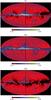 |
Fig. 2 M1, M2a, and M2b versions of NICER extinction maps. The colour scale is linear with respect to AJ. |
The latitude dependence of AJ is better visible in Fig. 3, which plots the median extinction against the latitude. The left frame shows how the extinction in the M2a maps rises towards the Galactic mid-plane, the profile being almost identical on the two hemispheres. On the other hand, the latitude profiles of M2b version are flat with values close to zero. In other words, in this case the reference colours are very close to the stellar colours reddened by the average extinction at each latitude. In principle, M2b represents the correct reference colours for a very nearby object whose extinction is seen above the average Galactic background. Because of the strong spatial variations of column densities, this is almost never precisely the case.
Figure 3b shows the also variations of the M2a maps where map is constructed using only the stars that are either below or above the median value of AJ of all stars within the smoothing kernel. The maps are at 3′ resolution. At high latitudes, the values are mostly noise and the selection of either low extinction or high extinction stars results in a significant bias, ΔAJ ~ 0.5 mag. Near the plane, the steeper rise of the AJ>median map should also have physical reasons related to unresolved high column density structures. Furthermore, when stars and extincting structures are mixed along LOS, AJ<median favours nearby clouds, resulting in larger scale height.
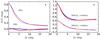 |
Fig. 3 Comparison of median NICER AJ profiles as function of Galactic latitude. Frame a) compares M2a (thin lines) and M2b maps (thick lines) for the profiles at positive (blue lines) and negative (red lines) Galactic latitudes. Frame b) shows comparison of M2a maps constructed using those stars that have values below (thin lines) or above (thick lines) the median AJ of all stars within the smoothing kernel. |
All extinction map versions (M1, M2a, M2b) should provide relatively similar measurements of local relative AJ changes. This is because the J − H and H − K reference values have a much weaker effect on AJ differences than on their absolute values. Figure 4 shows the correlations between the M2a and M2b extinction maps in a 10° × 10° region in Taurus. The two maps have an offset of ΔAJ = − 0.12 mag relative to each other but the slope of the linear correlation is close to one. The slope of an unweighted least squares fit is 0.98 but a slope 1.0 gives an almost perfect fit up to the highest AJ values. The small non-linearity (the least squares fit underestimating the values at the highest extinction) is caused by the difference of the M2a and M2b reference colours that changes as a function of latitude. However, above | b | ~ 10° the effect is already almost unnoticeable, apart from the zero point differences that makes the appearance of the two all-sky maps quite different near the plane.
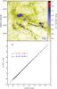 |
Fig. 4 Extinction map of Taurus and the correlation between the M2a and M2b estimates within the field. The scatter plot includes all pixels of the image (black dots). The red dashed line is the least squares fit and the blue line is a with slope set equal to one. |
5. Discussion
We have used the 2MASS survey stars to calculate all-sky NICER and NICEST maps at 3.0′, 4.5′, and 12.0′ resolution, all sampled onto Healpix pixels with NSIDE = 2048 (pixel size ~1.7′). We discuss below the possible uses of these maps and make comparisons with other all-sky extinction maps and detailed extinction mappings of selected clouds.
5.1. All-sky extinction estimates
The main motivation of this work was to provide a resource that can be easily checked for the presence of Galactic extinction. The maps do not and cannot measure the full extinction along the LOS and are instead weighted towards nearby structures.
There are previous estimates of extinction over the whole sky. Some of these “extinction” maps are, however, in fact derived from dust emission and are therefore measuring the total amount of dust along the LOS (Schlegel et al. 1998; Planck Collaboration XI 2014). First all-sky NIR extinction maps were presented by Dobashi (2011), together with an extensive catalogue of dark clouds detected in extinction. Those extinction maps were calculated based on J − H and H − K colours separately. The main improvement of the new NICER maps is that it makes an optimised combination of the colour information contained in the J, H, and K band magnitudes. This should result in an increase in S/N. Furthermore, the NICEST maps should give a more unbiased picture of the highest column density structures. By providing extinction maps in Healpix format, we hope that they will be useful for studies of extended regions of the sky or in studies involving large number of targets distributed over the whole sky.
We calculated NICER maps with three alternative definition of the reference colours that would correspond to zero extinction (see Sects. 3.2−3.3). These were M1 (average statistics at high latitudes, | b | > 60°) and two versions, M2a and M2b, based on Besançcon model of the Galactic distribution of stars with different intrinsic colours (M2a using the intrinsic colours, M2b colours further reddened by a simple model of diffuse extinction). The resulting extinction maps showed strong differences at large scales, especially near the Galactic plane. In spite of this, they give almost identical results for differential measures of extinction, if these are calculated over fields no larger than a few degrees. Near the Galactic plane the zero point of the extinction scale is not well defined because of the unknown mixture of stars and dust along the LOS. This ambiguity could be resolved only with knowledge of the 3D distribution of the stars and the ISM.
We believe the all-sky maps to be useful in many studies, at least as the first step towards more in-depth analysis of the local stellar populations and the reddening of their colours. The NICER maps (M1, M2a, M2b) and NICEST map (M1 version) are available on the web1. The site also includes NICER maps computed based on the stars below and above the median AJ of all stars in the beam. These may be useful in estimating the robustness of the extinction estimates. In the Galactic plane, they may also reveal distinct structures that might be located at different distances along the LOS (see Fig. 5). However, to actually prove the distance differences, more work is needed on the actual 3D distribution of the dense clouds (cf Marshall et al. 2009).
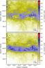 |
Fig. 5 Comparison of extinction maps using stars below (frame a)) or above (frame b)) the median extinction of all stars within the beam. Figures show a 6° × 6° field centred at Galactic coordinates (l, b) = (21.0, +0.0) degrees. The spatial resolution of the maps is 3′ and we have applied offsets to set the minimum of both maps at AJ ≈ 0 mag. |
5.2. Comparison with other NICER and NICEST maps
We compared our all-sky maps with some previously published extinction maps. As shown in Sect. 4, in a small field the different versions of extinction maps (M1, M2a, M2b) are very similar, with the exception of the AJ zero point. Therefore, we carry out the comparison using the M2a map only.
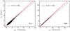 |
Fig. 6 Comparison at 6′ resolution of the M1 maps and the NICER maps of Perseus and Ophiuchus regions available at the COMPLETE web site. In Ophiuchus a half degree radius region centred at (l, b) = (351.9, 15.1) is affected by artefacts and is omitted from the plot. |
The COMPLETE data releases include a 9 × 12 degree NICER extinction map of the Perseus region, with a pixel size of 2.5′ and a spatial resolution of 5.0′2, and a 9 × 8 degree NICER map of Ophiuchus, with a spatial resolution of 3′ and a pixel size of 1.5′3. Figure 6 compares these with our M2a map. We resampled our data onto the pixels of the COMPLETE maps, and, to reduce the scatter resulting from the resampling, all data were convolved to a final spatial resolution of 6.0′.
The overall correspondence is good, the fitted least squares lines having a slope ~1.1 in both fields. The ~10% difference in the scaling can be explained by the adoption of a slightly different extinction curves (transformation from AJ to AV). Part of the scatter in Fig. 6 can be attributed to the different resolution of the original data and the uncertainty of the convolution for maps sampled at steps near the actual resolution. The relation of M2a vs. COMPLETE is well fitted by a linear relation up to the highest extinctions. In the correlation with M1 map (not shown) the slopes are identical but the scatter is somewhat smaller. The residual rms values were 0.13 mag and 0.11 mag instead of 0.18 mag and 0.13 mag (Perseus and Ophiuchus, respectively). This suggests that part of the dispersion originates because the reference colours in the M2a map change slowly across the field while they were probably kept constant in the case of the COMPLETE maps. However, the convolution of our data (originally at 3.0′ resolution but sampled only on ~1.7′ pixels) stands for most of the scatter in Fig. 6.
NICER and NICEST extinction maps of the Pipe Nebula are available on the web4 (see Lombardi et al. 2006). These maps have a resolution of 1.0′ and a pixel size of 30″. Figure 7 shows the comparison between this NICER map (“reference maps”, convolved to 3.0′ resolution) and our M1 maps calculated with NICER and NICEST methods. The zero point difference of ~0.12 mag is again related to the different assumption of the reference colours. Because the comparison is using NIR extinction AK, the scale should not be sensitive to the adopted extinction law.
The overall match is good but, compared to the reference map, our NICER estimates are systematically lower at high AK. This remains true even relative to a fit with slope forced to the value of one. Our map was calculated directly at the 3.0′ resolution and, therefore, suffers from higher bias because there are more column density variations within the beam. Using the NICEST method, most of the bias disappears. Thus, these errors indeed appear to be caused by small scale structures. Compared to the reference map, the overall scatter is reduced also in regions of lower extinction. The rms values of the difference are 0.015 and 0.011 mag, for Fig. 7a and b, respectively, significantly smaller than in the case of the Perseus and Ophiuchus fields because the comparison was done using directly our values on the original Healpix pixels, carrying out convolution only on the reference data that were well sampled.
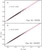 |
Fig. 7 Comparison at 3′ resolution of our M1 NICER map and the NICER map ( |

In the comparison, it is useful to look also at individual structures in the maps. Figure 8 shows a detail of the Pipe extinction map with two compact clumps. The comparison of the NICER and NICEST reference maps shows that NICEST method recovers (when examined at 3.0′ resolution, frame b) almost 20% higher peak values of extinction. Similarly, our M1-NICER map, being calculated at 3′ resolution instead of the 1′ resolution, shows peak values that are lower by a similar amount (frame c). M1-NICEST is much closer to the peak values of the reference NICER map. This shows that NICEST is able to compensate for much of the bias (almost all of the bias between 1′ and 3′ maps). In fact, Fig. 8d shows some negative residuals at the location of the extinction peaks. Thus, our NICEST estimates calculated at 3′ resolution are remarkably between the NICER and NICEST estimates calculated at 1′ resolution. Of course, even NICEST cannot replace all the information that is lost in the initial spatial averaging of the extinction estimates of individual stars. In particular, if some high column density regions are completely void of background stars, calculated extinction estimates are still only a lower limit of the true peak extinction.
In Fig. 8c and d some hatch pattern can be seen. This is because, unlike in Fig. 7, we have resampled our Healpix maps onto the pixels of the reference maps. Because the original M1 maps are defined on Healpix pixels with a size of 1.7′, after convolution the residual maps show artificial small scale structure. It would be better to resample the higher resolution data onto the pixels of the lower resolution data (as in Fig. 7) or, preferably, to have better sampling of all data. However, at the next higher resolution, NSIDE = 4096, the files would four times larger. This would diminish the practical usability of the maps, with little practical improvement. For the lower resolutions of 4.5′ and 12′, the sampling is more adequate.
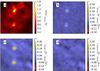 |
Fig. 8 A detail of the Pipe extinction maps. Frame a) shows the 1′ resolution NICER reference map (Lombardi et al. 2006) convolved to 3′ resolution. The other frames show relative differences between: Lombardi et al. NICEST and NICER maps (frame b); both convolved from 1′ to 3′), M1-NICER with the original resolution of 3′ and Lombardi et al. NICER convolved to the same resolution (frame c)), and M1-NICEST with the original resolution of 3′ and Lombardi et al. NICER convolved to the same resolution (frame d)). |
6. Conclusions
We have calculated all-sky extinction maps with 2MASS catalogue stars and using both NICER and NICEST methods. Calculations have been repeated with different assumptions of the reference colours corresponding to zero extinction. The analysis of the extinction estimates and comparison with extinction maps already available for some regions, we arrive at the following conclusions.
-
The appearance of the all-sky extinction map depends on the assumptions of reference colours, which are not well defined when stars and dust are intermixed along the LOS. However, the relative extinction estimates always agree very well when calculated for fields no larger than a few degrees in size.
-
The comparison carried out with extinction maps published for Taurus, Perseus, Ophiuchus, and Pipe Nebula regions shows good agreement. This suggests that extinction structures can be mapped relatively precisely without an in-depth analysis of the stellar populations in the field.
-
Because of small-scale column density variations, NICER maps underestimate at highest column densities the beam-averaged extinction. However, comparison with higher resolution maps showed the NICEST method to be effective in reducing this bias.
COMPLETE team, “2MASS Final Perseus Extinction Map”, http://hdl.handle.net/10904/10080 V2.
COMPLETE team, “2MASS Final Ophiuchus Extinction Map”, http://hdl.handle.net/10904/10081 V2.
Lombardi, Marco; Alves, Joao; Lada, Charles J., 2014, “2MASS extinction map of the Pipe Nebula”, http://dx.doi.org/10.7910/DVN/25112 Harvard Dataverse Network V3.
Acknowledgments
This publication makes use of data products from the Two Micron All Sky Survey, which is a joint project of the University of Massachusetts and the Infrared Processing and Analysis Center/California Institute of Technology, funded by the National Aeronautics and Space Administration and the National Science Foundation. M.J. acknowledges the support of the Academy of Finland Grant No. 250741. M.J. acknowledges the Observatoire Midi-Pyrenees (OMP) in Toulouse for its support for a 2 months stay at IRAP in the frame of the “OMP visitor programme 2014”, during which time this work was initiated.
References
- Alves, J., Lombardi, M., & Lada, C. J. 2014, A&A, 565, A18 [NASA ADS] [CrossRef] [EDP Sciences] [Google Scholar]
- Cambresy, L., Epchtein, N., Copet, E., et al. 1997, A&A, 324, L5 [NASA ADS] [Google Scholar]
- Cambrésy, L., Boulanger, F., Lagache, G., & Stepnik, B. 2001, A&A, 375, 999 [NASA ADS] [CrossRef] [EDP Sciences] [Google Scholar]
- Cambrésy, L., Beichman, C. A., Jarrett, T. H., & Cutri, R. M. 2002, AJ, 123, 2559 [NASA ADS] [CrossRef] [Google Scholar]
- Cardelli, J. A., Clayton, G. C., & Mathis, J. S. 1989, ApJ, 345, 245 [NASA ADS] [CrossRef] [Google Scholar]
- Davenport, J. R. A., Ivezić, Ž., Becker, A. C., et al. 2014, MNRAS, 440, 3430 [NASA ADS] [CrossRef] [Google Scholar]
- Dobashi, K. 2011, PASJ, 63, 1 [NASA ADS] [CrossRef] [Google Scholar]
- Dobashi, K., Uehara, H., Kandori, R., et al. 2005, PASJ, 57, 1 [Google Scholar]
- Dobashi, K., Marshall, D. J., Shimoikura, T., & Bernard, J.-P. 2013, PASJ, 65, 31 [NASA ADS] [Google Scholar]
- Górski, K. M., Hivon, E., Banday, A. J., et al. 2005, ApJ, 622, 759 [NASA ADS] [CrossRef] [Google Scholar]
- Juvela, M., Ristorcelli, I., Marshall, D., & et al. 2015, A&A, 584, A94 [NASA ADS] [CrossRef] [EDP Sciences] [Google Scholar]
- Lada, C. J., Lada, E. A., Clemens, D. P., & Bally, J. 1994, ApJ, 429, 694 [NASA ADS] [CrossRef] [Google Scholar]
- Lombardi, M. 2009, A&A, 493, 735 [NASA ADS] [CrossRef] [EDP Sciences] [Google Scholar]
- Lombardi, M., & Alves, J. 2001, A&A, 377, 1023 [NASA ADS] [CrossRef] [EDP Sciences] [Google Scholar]
- Lombardi, M., Alves, J., & Lada, C. J. 2006, A&A, 454, 781 [NASA ADS] [CrossRef] [EDP Sciences] [Google Scholar]
- Lombardi, M., Lada, C. J., & Alves, J. 2008, A&A, 489, 143 [NASA ADS] [CrossRef] [EDP Sciences] [Google Scholar]
- Lombardi, M., Lada, C. J., & Alves, J. 2010, A&A, 512, A67 [NASA ADS] [CrossRef] [EDP Sciences] [Google Scholar]
- Lombardi, M., Alves, J., & Lada, C. J. 2011, A&A, 535, A16 [NASA ADS] [CrossRef] [EDP Sciences] [Google Scholar]
- Lombardi, M., Bouy, H., Alves, J., & Lada, C. J. 2014, A&A, 566, A45 [NASA ADS] [CrossRef] [EDP Sciences] [Google Scholar]
- Marshall, D. J., Joncas, G., & Jones, A. P. 2009, ApJ, 706, 727 [NASA ADS] [CrossRef] [Google Scholar]
- Padoan, P., Cambrésy, L., & Langer, W. 2002, ApJ, 580, L57 [NASA ADS] [CrossRef] [Google Scholar]
- Planck Collaboration XI. 2014, A&A, 571, A11 [NASA ADS] [CrossRef] [EDP Sciences] [Google Scholar]
- Robin, A. C., Reyle, C., Fliri, J., et al. 2014, A&A, 569, A13 [NASA ADS] [CrossRef] [EDP Sciences] [Google Scholar]
- Rowles, J., & Froebrich, D. 2009, MNRAS, 395, 1640 [NASA ADS] [CrossRef] [Google Scholar]
- Schlegel, D. J., Finkbeiner, D. P., & Davis, M. 1998, ApJ, 500, 525 [NASA ADS] [CrossRef] [Google Scholar]
- Skrutskie, M., Cutri, R., Stiening, R., et al. 2006, Aj, 131, 1163 [NASA ADS] [CrossRef] [Google Scholar]
- Wang, S., & Jiang, B. W. 2014, ApJ, 788, L12 [NASA ADS] [CrossRef] [Google Scholar]
All Figures
|
Fig. 1 Six versions of all-sky maps of the average J − H (left frames) and H − K (right frames) colours. The first three are based on observed 2MASS sources (frames a)−c)) and the last three (frames d), f)) on stars simulated with the Besançon model. See text for details. The labels M1, M2a, and M2b refer to extinction maps where the corresponding data are used as reference colours. |
| In the text | |
|
Fig. 2 M1, M2a, and M2b versions of NICER extinction maps. The colour scale is linear with respect to AJ. |
| In the text | |
|
Fig. 3 Comparison of median NICER AJ profiles as function of Galactic latitude. Frame a) compares M2a (thin lines) and M2b maps (thick lines) for the profiles at positive (blue lines) and negative (red lines) Galactic latitudes. Frame b) shows comparison of M2a maps constructed using those stars that have values below (thin lines) or above (thick lines) the median AJ of all stars within the smoothing kernel. |
| In the text | |
|
Fig. 4 Extinction map of Taurus and the correlation between the M2a and M2b estimates within the field. The scatter plot includes all pixels of the image (black dots). The red dashed line is the least squares fit and the blue line is a with slope set equal to one. |
| In the text | |
|
Fig. 5 Comparison of extinction maps using stars below (frame a)) or above (frame b)) the median extinction of all stars within the beam. Figures show a 6° × 6° field centred at Galactic coordinates (l, b) = (21.0, +0.0) degrees. The spatial resolution of the maps is 3′ and we have applied offsets to set the minimum of both maps at AJ ≈ 0 mag. |
| In the text | |
|
Fig. 6 Comparison at 6′ resolution of the M1 maps and the NICER maps of Perseus and Ophiuchus regions available at the COMPLETE web site. In Ophiuchus a half degree radius region centred at (l, b) = (351.9, 15.1) is affected by artefacts and is omitted from the plot. |
| In the text | |
|
Fig. 7 Comparison at 3′ resolution of our M1 NICER map and the NICER map ( |
| In the text | |
|
Fig. 8 A detail of the Pipe extinction maps. Frame a) shows the 1′ resolution NICER reference map (Lombardi et al. 2006) convolved to 3′ resolution. The other frames show relative differences between: Lombardi et al. NICEST and NICER maps (frame b); both convolved from 1′ to 3′), M1-NICER with the original resolution of 3′ and Lombardi et al. NICER convolved to the same resolution (frame c)), and M1-NICEST with the original resolution of 3′ and Lombardi et al. NICER convolved to the same resolution (frame d)). |
| In the text | |
Current usage metrics show cumulative count of Article Views (full-text article views including HTML views, PDF and ePub downloads, according to the available data) and Abstracts Views on Vision4Press platform.
Data correspond to usage on the plateform after 2015. The current usage metrics is available 48-96 hours after online publication and is updated daily on week days.
Initial download of the metrics may take a while.