| Issue |
A&A
Volume 567, July 2014
|
|
|---|---|---|
| Article Number | A32 | |
| Number of page(s) | 11 | |
| Section | Interstellar and circumstellar matter | |
| DOI | https://doi.org/10.1051/0004-6361/201322945 | |
| Published online | 07 July 2014 | |
Grain growth in the envelopes and disks of Class I protostars ⋆
1
European Southern Observatory (ESO),
Karl-Schwarzschild-Strasse 2,
85748
Garching,
Germany
e-mail:
This email address is being protected from spambots. You need JavaScript enabled to view it.
2
Università degli Studi di Milano, Dipartimento di
Fisica, via Celoria
16, 20133
Milano,
Italy
3
INAF – Osservatorio Astrofidico di Arcetri, Largo E. Fermi 5,
50125
Firenze,
Italy
4
Excellence Cluster Universe, Boltzmannstr. 2, 85748
Garching,
Germany
5
Department of Astronomy, California Institute of
Technology, MC
249-17, Pasadena
CA
91125,
USA
6
Max-Planck-institute für extraterrestrische Physik,
Giessenbachstraße, 85748
Garching,
Germany
7
Australia Telescope National Facility, PO Box 76,
NSW 1710
Epping,
Australia
8
Harvard-Smithsonian Center for Astrophysics, 60 Garden Street,
Cambridge
MA
02138,
USA
9
School of Cosmic Physics, Dublin Institute for Advanced Studies,
31 Fitzwilliam Place,
2
Dublin,
Ireland
Received:
30
October
2013
Accepted:
1
May
2014
Abstract
We present new 3 mm ATCA data of two Class I young stellar objects (YSOs) in the Ophiucus star forming region: Elias29 and WL12. For our analysis we compare them with archival 1.1 mm SMA data. In the (u,v) plane the two sources present a similar behavior: a nearly constant non-zero emission at long baselines, which suggests the presence of an unresolved component and an increase of the fluxes at short baselines, related to the presence of an extended envelope. Our data analysis leads to unusually low values of the spectral index α1.1−3 mm, which may indicate that mm-sized dust grains have already formed both in the envelopes and in the disk-like structures at such early stages. To explore the possible scenarios for the interpretation of the sources we perform a radiative transfer modeling using a Monte Carlo code, in order to take into account possible deviations from the Rayleigh-Jeans and optically thin regimes. Comparison between the model outputs and the observations indicates that dust grains may form aggregates up to millimeter size already in the inner regions of the envelopes of Class I YSOs. Moreover, we conclude that the embedded disk-like structures in our two Class I YSOs are probably very compact, in particular in the case of WL12, with outer radii down to tens of AU.
Key words: circumstellar matter / opacity / radiative transfer / protoplanetary disks / stars: protostars / dust, extinction
Appendices are available in electronic form at http://www.aanda.org
© ESO, 2014
1. Introduction
Stars are formed out of the gas present in dense molecular clouds. In particular small-scale cores (with sizes on the order of 0.1 pc and estimated lifetime ~106 yr) within molecular clouds have been identified as the first stage of star formation (see review by Bergin & Tafalla 2007). The new-born protostars are initially embedded in rotating and collapsing envelopes made of cold gas and dust, which form in those cores. The material is gradually accreting from the envelopes onto the central objects through circumstellar disks, which form because of the conservation of angular momentum. Disks are thought to be the birthplace of planets. For the formation of rocky planets like our Earth, and probably also for rocky cores of giant planets, the dust component has to grow from grains of interstellar medium (ISM) of a few submicrons in diameter (Mathis et al. 1977) into bodies that are thousands of kilometers in diameter. During the first stages of the grain growth process gas and dust interact, leading the solid particles to collide and finally to aggregate (see the extensive reviews in Beckwith et al. 2000; Natta et al. 2007; Testi et al. 2013).
Young stellar objects (YSOs) are classified according to the slope of their spectral energy distributions (SEDs), usually in the range of wavelengths from 2.2 μm to 20 μm. Initially YSOs were studied in the infrared (IR; Lada 1987), and were classified as Class I, Class II, and Class III YSOs, depending on their near-infrared (NIR) slope. Subsequently, Class 0 YSOs were also defined observationally by André et al. (1993).
This observational classification is usually interpreted as an evolutionary sequence. In particular Class 0 YSOs are considered to be the first stage, when the prostostar is still completely embedded in its envelope that absorbs and reemits the radiation from the central star and disk (and Menv ≫ Mproto−⋆). They evolve towards the Class I phase, where the envelope is partially dissipated (Menv ≲ Mproto−⋆) and the emission from the primordial disk can be better separated from that of the envelope. In the Class II stage the envelope has disappeared, the central pre-main-sequence star (PMS) becomes optically visible, and the disk is optically thick in the IR and optically thin in the mm. Then the source enters in the Class III phase, where the more evolved PMS may be surrounded by a tenuous, optically thin disk and planets or a so-called debris disk may be present.
An interesting question is when and where dust grains begin to grow during this evolutionary sequence. Observational results indicate that nearly all the disks in the Class II phase contain dust grains with sizes of at least 1 mm in their outer regions (see, e.g., Ricci et al. 2010a, and references therein), independent of mass and environment (we note, however, the interesting case of the Chamaeleon I region by Ubach et al. 2012). This shows that the formation of these large grains has to be very rapid, occurring before a YSO enters the Class II stage, in the early phases of disk formation or possibly even in the collapsing envelopes.
Pagani et al. (2011) present preliminary evidence of grain growth up to ~1 μm already within dense cores, through the detection of an IR core-shine, i.e, strong scattering of background radiation due to micron-sized grains within the core. Similar levels of grain growth have also been derived from the study of the extinction law in Perseus dense cores (Foster et al. 2013). Moreover, according to the studies by Jørgensen et al. (2007), Kwon et al. (2009), and Chiang et al. (2012) there are possible indications from millimeter observations that even larger grains are present in the central regions of the evelopes surrounding Class 0 protostars. There is, however, a caveat in studying Class 0, i.e., the emission may come from regions that are optically thick at submillimeter wavelengths.
Class I YSOs represent the transition phase between cores and disks, where both the envelope and the disk are detectable and the two different components can be separated more easily than in Class 0 YSOs. They are well suited to studying the first stages of grain growth and to constraining the initial condition for the evolution of protoplanetary disks.
The radiative emission by dust grains depends on the typical grain size. Dust continuum emission in the millimeter allows us to place constraints on dust properties of disks and envelopes in nearby star forming regions (SFRs). Unlike optical and infrared studies that are mostly sensitive to growth up to micron-sized particles, millimeter wavelengths allow us to test the presence of mm/cm-sized grains. At these long wavelengths the emission of the disk is mostly optically thin and, as a consequence, the spectral index αmm of the SED (Fν ≈ ναmm) carries the information on the spectral index βmm of the dust opacity coefficient (κν ≈ νβmm; see Beckwith & Sargent 1991; Testi et al. 2001; Natta et al. 2007; Draine 2006). In particular, for the approximate case of optically thin emission in the Rayleigh-Jeans regime, αmm = βmm + 2, ISM-like particles are usually characterized by βmm ~ 1.7 (and αmm ~ 3.5), while larger mm/cm-sized grains have lower values of βmm and αmm (Draine 2006). This relation between αmm and βmm holds independent of the geometry of the system, i.e. also in the envelope Fν ~ ν2+βmm. Therefore, multi-wavelength observations of YSOs in the (sub-)millimeter can reveal the presence of mm/cm-sized pebbles in disks and in envelopes (Testi et al. 2013).
In this paper we present new mm and cm observations of Elias29 and WL12, two Class I YSOs in the ρ Ophiuchi SFR, with the aim of constraining the grain size distribution on the disk and envelope of each object separately. These objects have been studied previously with the Submillimeter Array (SMA) at 1.1 mm by Jørgensen et al. (2009). In Sect. 2 we present our new observations of both Elias29 and WL12 with the Australian Telescope Compact Array (ATCA) at 3 mm, 3 cm and 6 cm. Then, in Sects. 3 and 4 we present the results of the data reduction process and a first-order analysis of the dataset. A more accurate analysis is presented in Sect. 5 and discussed in Sect. 6. Finally, we summarize our results in Sect. 7.
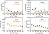 |
Fig. 1 Visibility amplitudes expressed in jansky against the u–v distances in kλ.The data points give the amplitudes per bin. The data are binned in annuli according to u–v distance. In the top panels we present the amplitudes of Elias29: in the left panel, the archival 1.1 mm SMA dataset (Jørgensen et al. 2009), and in the right panel the new 3 mm ATCA dataset. In the bottom panels we plot the same for WL12. The histograms give the expected amplitudes for zero signal. The open triangles at zero u–v distance give the zero spacing 1.1 mm fluxes, interpolated between 850 μm and 1.25 mm single-dish fluxes (Lommen et al. 2008; Jørgensen et al. 2009). The orange lines are the best fits of the observed emission, obtained using a combination of a two-layer disk model (Chiang & Goldreich 1997; Dullemond et al. 2001) surrounded by a power-law density envelope. We used the Monte Carlo radiative transport model RADMC-3D (Dullemond & Dominik 2004) to compute the emission from the envelope. The separate contributions given by the disk and the envelope are plotted with the dotted and dashed lines, respectively |
2. Observations
2.1. Selection of sources
We selected two sources located in the ρ Ophiuchi SFR, taken to be at a distance D = 125 ± 25 pc (de Geus et al. 1989; Lombardi et al. 2008): Elias29 and WL12. Their infrared colors, their bolometric luminosities, and their temperatures were obtained with Spitzer photometry from the “Cores to Disk” legacy program (Evans et al. 2009). The two sources have similar bolometric temperatures, Tbol = 391 K for Elias29 and Tbol = 440 K for WL12, while their bolometric luminosities are estimated to be Lbol = 13.6 L⊙ and Lbol = 2.6 L⊙, respectively.
The two sources have been classified as Class I from the slope of their SED in the near- and mid-infrared (Evans et al. 2009). They have been also observed at 1.1 mm with SMA within the PROSAC program (Jørgensen et al. 2009), and in particular Elias 29 was studied by Lommen et al. (2008), who gave an estimate of the star, disk, and envelope masses (Table 1).
2.2. ATCA observations
The observations were performed with ATCA using the CABB wideband correlator between July 2011 and September 2011 in three variations of its hybrid configurations: H75, H168 and H214. Two 2 GHz wideband centered at 93.0 and 95.0 GHz were used for the 3 mm observations, while for 3 and 6 cm we used 2 GHz wideband centered at 9.0 and 5.0 GHz, respectively. The projected baselines provided were in the range 7–79 kλ for Elias29, while they were 7–98 kλ for WL12. Calibration was done using the MIRIAD package (Sault et al. 1995). The sources 1253-055 and 1622-297 served as band-pass and phase calibrators and the absolute fluxes were calibrated on Uranus.
2.3. SMA observations
In our analysis we also made use of archival 1.1 mm data (frequencies: 267 and 277 GHz), obtained with SMA within the PROSAC program (Jørgensen et al. 2009). The observations were performed between May 2006 and July 2007 in two variations of SMA compact configuration. The projected baselines were from 5.9 kλ to 64 kλ for Elias29 and from 9 kλ to 104 kλ for WL12.
Parameters from literature.
3. Results
3.1. Results at mm wavelengths
The visibility amplitudes at 3 mm are plotted in the right panels of Fig. 1 as a function of projected baselines, 7–60 kλ for Elias29 and 7–70 kλ for WL12. We also report the visibility amplitudes obtained with the archival 1.1 mm SMA data (left panels), whose baselines range from 5.9 kλ to 60 kλ for Elias29 and from 9 kλ to 70 kλ for WL12. The observations at 3 mm were taken using a range of u–v distances chosen to overlap with those of the SMA dataset. The smallest physical scales that we are able to resolve at both 1.1 and 3 mm are around 400 AU, while the short baselines correspond to scales larger than a few thousands of AU.
In the case of Elias29 the emission at 1.1 mm rises at the shortest baselines, indicating the presence of an envelope, as already concluded by Lommen et al. (2008). The u–v distances at which the fluxes start to increase correspond to physical scales too large to be related with a resolved disk. The increasing trend is not as evident in the 3 mm plot, because of the lack of data for projected baselines shorter than 7 kλ. At larger u–v distances, on the other hand, the emission is approximately constant in both datasets, showing the presence of an unresolved source, i.e. a disk-like structure. Similar behavior is found for WL12, even if the rise is less steep at the short baselines.
3.2. Estimated ionized gas contribution
We obtained a clear detection of the two sources at 3 mm (Figs. 2 and 3). On the other hand, we did not detect either of the two sources at 3 cm and at 6 cm. Dzib et al. (2013) have recently published a deep cm continuum survey of the ρ-Ophiuchi SFR using the VLA. They detected Elias 29 ( J162709.41-243719.0), but not WL12. Their upper limits at 6 and 4 cm are a factor of ~10 lower than ours. The measured cm-wave fluxes of Elias 29 are ~0.25 mJy at 6 cm and ~0.36 mJy at 4 cm, with a spectral index of ~0.7. The source is reported to be variable at the 30% level. The extrapolated contribution of the gas emission at 3 mm would be ~2 mJy, about 20% of the total flux. We decided not to subtract this possible contribution from the 3 mm fluxes we measured, reported in the next paragraph, because of the source variability and because our observations and those of Dzib et al. (2013) are not simultaneous. The VLA observations were obtained in the period February–May 2011, while our own ATCA data were acquired in June, August, and September 2011. The time difference between the various epochs is not large, but Dzib et al. (2013) report variability on a monthly timescale.
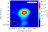 |
Fig. 2 Elias29 map: detection of the source at 3 mm. The total flux of the source at 3 mm is 10.36 mJy, with a 3σ rms of 0.18 mJy. |
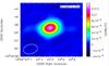 |
Fig. 3 WL12 map: detection of the source at 3 mm. The total flux of the source at 3 mm is 17.48 mJy, with a 3σ rms of 0.22 mJy. |
To provide a worst case scenario for the contamination of the gas emission at 3 mm we use
our simultaneous upper limits at 3 and 6 cm. The most efficient way to produce ionized gas
which can contaminate the dust thermal emission at 3 mm is given by the presence of a
stellar wind (i.e. mass ejection from the star). In this case the radio spectrum is found
to vary as Fν ∝
ν0.6 (Panagia & Felli 1975), while, for example, the free-free emission coming
from an optically thin HII region would give Fν ∝
ν-0.1 (Mezger 1970). Using the 3σ limits at 3 and 6 cm (Table 2) we then compute the maximum possible contribution
from an ionized wind at 3 mm. The extrapolated contributions from ionized gas at 3 mm are
 mJy for Elias29 and
 mJy for WL12, less than
36% and 20% of the observed total fluxes at 3 mm
respectively.
mJy for WL12, less than
36% and 20% of the observed total fluxes at 3 mm
respectively.
In Sect. 4 we use our upper limits to estimate the impact of the free-free emission on the measurement of the spectral index of the dust emission; this choice corresponds to a larger maximum estimated contamination and is thus a conservative estimate.
4. Analysis
As a first-order analysis, we assume our sources to be composed of two elements, the envelope and the disk, whose emission are expected to be easily separable (see, e.g., Jørgensen et al. 2009). Since our observations do not allow us to resolve the disk (60 kλ are related to disk diameters on the order of almost 400 AU) we expect the disk amplitude to be constant (unresolved source), without changing appreciably with baseline length. On the other hand, we expect the envelope to be resolved and to dominate the emission on the largest detected scale. Therefore, its emission should be high at the small baselines and approach zero at the larger ones where the disk contribution is expected to dominate. An analysis of the SMA data similar to these suggested the presence of extended envelopes and compact disks around these two sources (see Lommen et al. 2008; Jørgensen et al. 2009), as it also has for other sources.
Source fluxes at different wavelengths.
For Elias29 in particular, the value of the amplitudes is constant within the errorbars
for baselines larger than 25 kλ both at 1.1 and 3 mm. We assume this to be the
emission coming from the embedded disk-like structure whose average values at the two
wavelengths are  and
and
 . These values were obtained
using a weighted average using the weights associated with the single observed visibilities.
For WL12 we make the same assumption, relating the disk contribution to the amplitudes at
baselines larger than 40 kλ. The disk average fluxes at the two wavelengths are
. These values were obtained
using a weighted average using the weights associated with the single observed visibilities.
For WL12 we make the same assumption, relating the disk contribution to the amplitudes at
baselines larger than 40 kλ. The disk average fluxes at the two wavelengths are
 and
and
 .
.
Under the optically thin assumption and the Rayleigh-Jeans approximation, given a
dual-frequency observation where the fluxes at the frequencies ν1 and
ν2
are F1 and F2,
β can be
easily obtained as  (1)Using the fluxes in the
same u–v ranges at 1 and 3 mm, we obtain therefore the average value of
β in the
disk, which is βdisk
= −0.16 ± 0.19 for Elias29 and βdisk = −0.47 ±
0.07 for WL12. These estimates assume that all the emission at 3 mm is
due to thermal dust emission. We can use the upper limits on the cm-wave emission (see Sect.
3.2) to estimate the maximum possible contribution of
the gas emission at 3 mm. If we assume that there is a compact gas component emission at a
level equivalent to the 3σ upper limit derived from our cm observations (Table
2), then the value of β in the disk becomes higher
for both sources:
(1)Using the fluxes in the
same u–v ranges at 1 and 3 mm, we obtain therefore the average value of
β in the
disk, which is βdisk
= −0.16 ± 0.19 for Elias29 and βdisk = −0.47 ±
0.07 for WL12. These estimates assume that all the emission at 3 mm is
due to thermal dust emission. We can use the upper limits on the cm-wave emission (see Sect.
3.2) to estimate the maximum possible contribution of
the gas emission at 3 mm. If we assume that there is a compact gas component emission at a
level equivalent to the 3σ upper limit derived from our cm observations (Table
2), then the value of β in the disk becomes higher
for both sources:  for
Elias29 and
for
Elias29 and  for WL12.
Second, we find an excess of emission at the very short baselines (i.e. from 6.9
kλ up to 10
kλ for
Elias29 and from 6.8 kλ up to 15 kλ for WL12), when subtracting the disk visibilities
from the total visibilities. The physical scales related to these u–v
distances range from around 2000 AU to 4000 AU. The excess values at these short
baselines are  and
and
 for
Elias29 and
for
Elias29 and  and
and
 for
WL12. The excesses, even if they are not very large in the ATCA datasets, are detected
especially in Elias29 and can be linked with the presence of an envelope in both sources.
This hypothesis is also supported by the single-dish fluxes extrapolated at 1.1 mm combining
1.25 mm fluxes (André & Montmerle 1994) and
850 μm fluxes
(Johnstone et al. 2004; Ridge et al. 2006) as done by Lommen et
al. (2008). They are shown by the open triangles in Fig. 1, and are substantially larger than the interferometer fluxes. They
indicate that extended emission is present around the compact component source picked up in
both the sources by the long baselines. This extended emission is due to the circumstellar
envelope, as discussed by Lommen et al. (2008) and
Jørgensen et al. (2009). Considering only the
interferometer fluxes at these very short baselines, using the same u–v
distance ranges at 1.1 and 3 mm, it is possible to obtain an average value of
β given by
the excess fluxes, accordingly with Eq. (1),
which are: βenv = 0.6
± 0.3 for Elias29 and βenv = 0.8 ± 0.7 for WL12. The errors on
β are
estimated following the procedure shown in Appendix A.
The uncertainties on the values of βenv are large, since the visibilities are
few and the signal-to-noise ratio is accordingly very low.
for
WL12. The excesses, even if they are not very large in the ATCA datasets, are detected
especially in Elias29 and can be linked with the presence of an envelope in both sources.
This hypothesis is also supported by the single-dish fluxes extrapolated at 1.1 mm combining
1.25 mm fluxes (André & Montmerle 1994) and
850 μm fluxes
(Johnstone et al. 2004; Ridge et al. 2006) as done by Lommen et
al. (2008). They are shown by the open triangles in Fig. 1, and are substantially larger than the interferometer fluxes. They
indicate that extended emission is present around the compact component source picked up in
both the sources by the long baselines. This extended emission is due to the circumstellar
envelope, as discussed by Lommen et al. (2008) and
Jørgensen et al. (2009). Considering only the
interferometer fluxes at these very short baselines, using the same u–v
distance ranges at 1.1 and 3 mm, it is possible to obtain an average value of
β given by
the excess fluxes, accordingly with Eq. (1),
which are: βenv = 0.6
± 0.3 for Elias29 and βenv = 0.8 ± 0.7 for WL12. The errors on
β are
estimated following the procedure shown in Appendix A.
The uncertainties on the values of βenv are large, since the visibilities are
few and the signal-to-noise ratio is accordingly very low.
Our inferred values of β for both the disks and the envelopes are surprisingly low if compared to typical values found in the ISM, as reported in the introduction. To investigate the possible explanations, proper radiative transfer modeling of both structures is needed, taking into account possible deviations from the Rayleigh-Jeans and optically thin regimes, which can affect the determined β values.
Estimated stellar parameters.
5. Modeling
The modeling approach used in this work consists in separating the disk+protostar system from the envelope, as extensively done in previous studies (e.g, Butner et al. 1994; Hogerheijde et al. 1999; Looney et al. 2003; Jørgensen et al. 2004, 2009). The disk+protostar system is modeled adopting the two-layer model by Dullemond et al. (2001), whose output spectrum is taken as the central source of heating in the envelope modeling. The envelope is modeled as done by Crapsi et al. (2008), using the Monte Carlo radiative transfer code RADMC-3D (Dullemond & Dominik 2004). Below we discuss in more detail the disk and the envelope models separately.
5.1. Disk models
We adopt the two-layer model of a flared disk heated by the central protostellar radiation by Chiang & Goldreich (1997), as developed by Dullemond et al. (2001). These models have been used by, e.g., Testi et al. (2003), Natta et al. (2004), and Ricci et al. (2010b) and we refer to these papers for a detailed description of the models.
First, in order to characterize a model we need to specify the properties of the central
heating source, approximated with a photosphere: its luminosity L⋆, its effective
temperature Teff, and its mass M⋆. We estimate
L⋆ = 13.6
L⊙, Teff = 4786 K,
and M⋆ = 3
M⊙ for Elias29 and L⋆ = 2.6
L⊙, Teff = 3980 K,
and M⋆ = 0.6
M⊙ for WL12, following the procedure
discussed in Appendix B. Then, a characterization of
the disk structure is needed, i.e. the inner and the outer radii Rin and
Rout, the disk inclination angle
i
(90° for an
edge-on disk), and the dust surface density profile, which for simplicity is assumed to be
a power law,  (2)where Σ0 is the surface dust density at
a radial distance of 1 AU from the central object and where we set p = 1, since the quality of
our data does not allow us to discriminate between different values of p. The value of
Σ0 was scaled to
accomodate the total disk mass Mdisk. The disk inclination angle is
assumed to be i =
60°, because the corresponding disk luminosity is equal to
the one obtained by averaging over all possible inclination angles (see, e.g., Butner et al. 1994).
(2)where Σ0 is the surface dust density at
a radial distance of 1 AU from the central object and where we set p = 1, since the quality of
our data does not allow us to discriminate between different values of p. The value of
Σ0 was scaled to
accomodate the total disk mass Mdisk. The disk inclination angle is
assumed to be i =
60°, because the corresponding disk luminosity is equal to
the one obtained by averaging over all possible inclination angles (see, e.g., Butner et al. 1994).
The mm-SED is not sensitive to Rin, which we then set equal to 0.25 AU. The measured fluxes at 1.1 and 3 mm are instead sensitive to the dust density, so that Rout and the mass of the dust in the disk Mdisk can be constrained by the observations (assuming a dust opacity and a gas-to-dust mass ratio). We fix gas/dust to 100 by mass and we explore the effects of using different prescriptions for κν depending on the dust size.
5.2. Envelope models
In order to model the envelopes of our sources we adopted the theoretical structure of a rotating and collapsing spheroid as derived by Ulrich (1976), and as done by Crapsi et al. (2008) and Lommen et al. (2008). This model assumes that matter crosses a spherical surface r0 at a uniform rate and then it falls freely, conserving angular momentum. The surface at r0 rotates uniformly.
The envelope density structure for a rotating and collapsing spheroid is given by
 (3)where Rrot is the
centrifugal radius of the envelope, ρ0 is the density in the equatorial
plane at the centrifugal radius and the quantity θ0 is the
solution of the parabolic motion of an infalling particle given by [r (cosθ0 −
cosθ) /(Rrotcosθ0sin2θ0)] = 1. Equation (3)
represents a free-falling envelope on large scales and flattened on smaller. On larger
scales it therefore matches the assumptions in Jørgensen
et al. (2009).
(3)where Rrot is the
centrifugal radius of the envelope, ρ0 is the density in the equatorial
plane at the centrifugal radius and the quantity θ0 is the
solution of the parabolic motion of an infalling particle given by [r (cosθ0 −
cosθ) /(Rrotcosθ0sin2θ0)] = 1. Equation (3)
represents a free-falling envelope on large scales and flattened on smaller. On larger
scales it therefore matches the assumptions in Jørgensen
et al. (2009).
The outer radius of the envelope is fixed to 50 000 AU, the value of the centrifugal radius Rrot is 300 AU as found by Lommen et al. (2008) for Elias29, while ρ0 is a free parameter used to adjust the envelope mass Menv. In our envelope models we do not include outflow cavities, as Lommen et al. (2008) did.
For each of the two sources, the temperature structure of the envelope was computed using the RADMC-3D code (Dullemond & Dominik 2004), implementing the envelope density structure of Eq. (3). The source of heating at the center was the disk-star system, whose emission was previously computed using the two-layered disk model (Dullemond et al. 2001) and the disk not included specifically in the 3D dust radiative transfer models used for the envelope structure. The source of heating has been implemented in a similar way to the one discussed in Butner et al. (1994).
5.2.1. Dust opacity
The dust opacity depends on grain sizes, shape and composition (e.g., Miyake & Nakagawa 1993; Pollack et al. 1994; Draine 2006). Estimates of the level of grain growth from the mm-SED can be made by making assumptions on the chemical composition and shape of the dust grains.
During the early stages of planet formation dust grains are thought to either stick or fragment, depending on their relative velocity. Therefore, it is important to consider a dust population characterized by a distribution of grains with different sizes. We adopt a truncated power law n(a) ∝ a− q, between a minimum and a maximum size, respectively amin and amax (see Birnstiel et al. 2011). In this paper, we consider the grains as having a spherical geometry, since the growth of small particles to larger ones (with sizes of ~1 mm) typically leads to compact structures, that are closer to spheres (Beckwith et al. 2000). When the chemical composition and the shape of the grains are fixed, the dust opacity law depends only on q, amin and amax.
We set amin ~ 0.1 μm, because grains are supposed to grow from submicron ISM-like grains (Mathis et al. 1977) and can be subject to collisional fragmentation, to a distribution in size of the grain population (Birnstiel et al. 2011). Moreover, amin can be set equal to a fixed value, since the dependence of the millimeter dust opacity on it is very weak, as long as amin ≪ 0.1 mm. We set q = 3 and therefore amax remains the only variable to determine. The dependence on q is discussed in Natta & Testi (2004). The values of the dust opacity per unit dust mass κν at 1.1 mm and 3 mm are 2.47 cm2 g-1 and 1.59 cm2 g-1, respectively.
5.3. Model fitting
Our aim is to find the set of parameters to simulate the sky brightness distribution that
best fits the observations. The free parameters for the disk are its mass Mdisk, its outer
radius Rout, and
 which
determines the disk dust opacity; for the envelope the free parameters are its mass
Menv and its dust opacity, i.e.
which
determines the disk dust opacity; for the envelope the free parameters are its mass
Menv and its dust opacity, i.e.
 .
.
Once the simulated images are produced, they need to be compared with the interferometric observations. To do that, we interpolate the model output images at the exact wavelengths of our observations.
It is not appropriate to compare the model images with the observed images, as the interferometer acts as a spatial filter. Therefore, it is necessary to simulate interferometric observaitons of the model images, to account for the interferometer primary beam attenuation and the filtering effect on the Fourier plane. To do this, we first multiply the model images with the primary beam attenuation pattern of the interferometer (assuming a Gaussian beam for both interferometers) and then we perform the Fourier ransform of the attenuated model images and sample them at the appropriate (u,v) locations in order to obtain simulated visibilities.
Our procedure starts with fitting the disk emission: using the two-layered disk model
(Dullemond et al. 2001) we vary Mdisk,
Rout, and
 to
reproduce together
to
reproduce together  and
and  .
In particular the three parameters need not only to reproduce the integrated fluxes at the
two frequencies, but also to take into account the interferometric data at the long
baselines (i.e. since the disks appear not resolved on the u–v plane, the
outer radii need to be Rout < 200 AU).
.
In particular the three parameters need not only to reproduce the integrated fluxes at the
two frequencies, but also to take into account the interferometric data at the long
baselines (i.e. since the disks appear not resolved on the u–v plane, the
outer radii need to be Rout < 200 AU).
Once the three parameters are found, we implement the output flux of the disk model as
the source of heating at the center of the envelope. Using the Monte Carlo radiative
transfer code RADMC-3D (Dullemond & Dominik
2004), we vary Menv and
 , in order
to reproduce at the same time the single-dish and the interferometric fluxes both at 1.1
mm and at 3 mm.
, in order
to reproduce at the same time the single-dish and the interferometric fluxes both at 1.1
mm and at 3 mm.
In Fig. 1 we present the best fit for the observed visibilities, both at 1.1 mm and 3 mm for Elias29 and WL12. Within the signal-to-noise ratio of the observations and the simplified models adopted, the simulated (u,v) profiles reproduce adequately the observed ones. The parameters of the models that provide a best match with the data are presented in Sect. 6 and in Table 4. The best models have been selected as to provide a reasonably good match with the data; a full χ2 minimization analysis is beyond the scope of this simplified modeling. We will, however, discuss the model uncertaintes below.
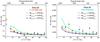 |
Fig. 4 Visibility amplitudes vs. u–v distances for Elias29 at both 1.1 and 3 mm. The orange line is our best fit of the data, while the blue and green lines represent two models obtained by decreasing and increasing the envelope mass, respectively. We note that these two models also fail to reproduce the single-dish flux at 1.1 mm (Lommen et al. 2008; Jørgensen et al. 2009), shown by the open triangle. |
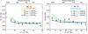 |
Fig. 5 Visibility amplitudes vs. u–v distances for WL12 at both 1.1 and 3 mm. The orange line is our best fit of the data, while the blue and green lines represent two models obtained by decreasing and increasing the envelope mass, respectively. We note that these two models also fail to reproduce the single-dish flux at 1.1 mm (Lommen et al. 2008; Jørgensen et al. 2009), shown by the open triangle. |
6. Discussion
6.1. Envelopes properties
Since our interferometric data allow us to probe only the inner envelope regions, i.e. R ≲ 3000 AU, with our simplified models we do not claim to give a detailed description of the whole envelope. For this reason we consider a large uniform envelope with a constant dust grain population, with the aim of reproducing the single-dish fluxes and the behavior of the interferometric data on the u–v plane. This approach is too simplistic to accurately model the outer envelope; one would need to compare more detailed models with observations at more compact baselines. Consequently, our models to not reproduce the full observed SEDs of Elias29 and WL12: this kind of study is beyond the scope of our work.
The models that provide the best match to our observations were computed using the
following parameters, reported also in Table 4; a
distribution of dust grains in the envelopes with maximum size
 mm for
both sources and inner envelope masses1Minn env
~ 0.03 M⊙ for Elias29 and Minn env ~ 0.04
M⊙ for WL12. To estimate the
uncertainties on the determination of the inner envelope masses, we show in Figs. 4 and 5 the effects
of changing this parameter. The orange line is our best match to the data, while the blue
and the green lines represent the predictions given by two models where we decreased and
increased the inner envelope mass in order to roughly reproduce (within 1σ) the observed
interferometric amplitudes. With this method we estimate an uncertainty in our derivation
of the inner envelope mass of the order of 50% (on top of the assumptions on the dust
opacity coefficient and the gas to dust ratio mentioned above). The predicted single-dish
fluxes at 1.1 mm are represented by the coloured rhombi at zero u–v
distances in the left panels. The values obtained with the increased- and
decreased-mass models highly overstimate and understimate the single-dish fluxes and are
shown by the open triangles.
mm for
both sources and inner envelope masses1Minn env
~ 0.03 M⊙ for Elias29 and Minn env ~ 0.04
M⊙ for WL12. To estimate the
uncertainties on the determination of the inner envelope masses, we show in Figs. 4 and 5 the effects
of changing this parameter. The orange line is our best match to the data, while the blue
and the green lines represent the predictions given by two models where we decreased and
increased the inner envelope mass in order to roughly reproduce (within 1σ) the observed
interferometric amplitudes. With this method we estimate an uncertainty in our derivation
of the inner envelope mass of the order of 50% (on top of the assumptions on the dust
opacity coefficient and the gas to dust ratio mentioned above). The predicted single-dish
fluxes at 1.1 mm are represented by the coloured rhombi at zero u–v
distances in the left panels. The values obtained with the increased- and
decreased-mass models highly overstimate and understimate the single-dish fluxes and are
shown by the open triangles.
We can constrain the level of grain growth in the envelopes within the framework of our physical but idealized collapsing rotating envelope models. For example, if we consider a dust grain size distribution in the envelope of Elias29 (see Fig. 6), with a maximum size of 1 μm we can reproduce the 1.1 mm observations, but we very significantly understimate the 3 mm fluxes. The observations directly constrain the frequency dependence of the dust opacity coefficient β, and we find β~ 0.5–1. If we use our dust model to infer the maximum grain size from this value of β, we would imply the presence of dust grains grown to millimeter-size aggregates. As discussed by many authors, while the exact maximum size of grains depends on the assumption of the geometry and composition of grains, it is very difficult to explain the measured values of β below 1 at millimeter wavelengths without invoking a significant growth of the dust aggregates (e.g., Natta & Testi 2004; Draine 2006; Banzatti et al. 2011).
Parameters derived from the modeling procedure.
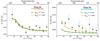 |
Fig. 6 Visibility amplitudes vs. u–v distances for Elias29 at both 1.1 and 3 mm. The orange line is our best fit of the data, obtained with a 2 M⊙ envelope, where grains have already grown up to mm size. The green line represents a model obtained with a 1.1 M⊙ envelope, with grains up to the micrometer size, in order to reproduce the 1.1 mm observations. It fails, however, to reproduce the 3 mm data. This shows that only the presence of already grown grains can give the dust an opacity able to reproduce the dual-frequency observations. |
The low values of β in our sources are compatible with those found by Tobin et al. (2013) in L1527 IRS. The fact that we find mm-sized grains in the envelope of Class I sources is also in agreement with the evidence of grown particles in the envelope of the Class 0 L1157-mm (Chiang et al. 2012). These findings are consistent with the timeline proposed by the latest meteoritic studies for the growth of solids in our own solar system: from chronological studies of solids found in meteorites, we know that the formation timescales of such mm-sized grains are similar to the median lifetimes of Class 0 and I (Connelly et al. 2012). Grain growth in cores and protostellar envelopes has been modeled by Ormel et al. (2009), although current models cannot easily explain growth at the level we are inferring. The results of our analysis show that grain growth up to mm-size occurred in Elias29 and WL12 at scales between 2000 AU and 4000 AU. In our envelope models, this corresponds to a range of number densities between 104 cm-3 and 105 cm-3. This is at least two orders of magnitude below the volume densities required by the models of Ormel et al. (2009) for grains to grow to millimeter sizes in reasonable timescales. The models require n> 106−107 cm-3 to form mm-sized grains on a timescale of 1 Myr. This discrepancy needs to be analysed in more detail, both observationally and on the modeling side.
The possibility that grains can grow up to mm-size already in the collapsing envelopes of Class 0 and I is a result that may have important implications on the initial conditions for the models of dust evolution in protoplanetary disks. This would imply that the grain growth process within the disk starts with mm-sized particles rather than with ISM-like grains as typically assumed by models of dust evolution in disks (Birnstiel et al. 2011). However, this would probably not lead to very different conclusions on the dust evolution in the disk, since grain growth is expected to be a very fast process in the disk environment.
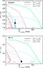 |
Fig. 7 Millimeter flux density vs. spectral index for disk models for Elias29 (top panel) and WL12 (bottom panel). The black dots show our ATCA data. Each line represents the prediction of disk models with the same disk outer radius and dust opacity spectral index β, but increasing disk mass from left to right. For Elias29 the observed flux and spectral index are consistent with both a small (R ~ 15 AU) optically thick disk, in which case we cannot constrain the dust properties, or a relatively large (R ~ 50–200 AU) optically thin disk populated with cm-sized pebbles. For WL12 the match between the observed data and the models suggests a very small and optically thick disk with a 30 AU radius. It is not possible to determine whether the grains are in the μm- , mm- or cm-sized regime . |
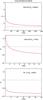 |
Fig. 8 Radial profile of the stability parameter Q. For Elias29 in the upper panel an extended disk model is assumed (Rout = 300 AU), while in the central panel a compact disk model is assumed (Rout = 15 AU). In the first case, in the outer regions of the disk Q approaches unity, showing marginal stability. In the second case, the value of Q drops below unity, showing the presence of strong gravitational instability. In the bottom panel a compact disk model is assumed (Rout = 30 AU) for WL12. In this case Q also assumes very low values, showing that prominent gravitational instability is present. |
6.2. Disk properties
For both sources the estimated value of αdisk and consequently of βdisk are very low. To compare these results with the predictions of disk models we plotted the spectral index vs. the millimeter flux density for our data and for a set of families of disk models in Fig. 7, following the method developed in Testi et al. (2001). Different line colours represent the predictions of disk models with different disk outer radii. For each line the disk mass increases from left to right and accordingly also the mass surface density and the optical depth also increase. For smaller disk masses the disk is optically thin and the flux increases when the mass increases. When the optical depth becomes ≫1, the disk emission becomes less and less dependent on the disk mass and the spectral index assumes lower values. This explains the trend of the lines in the α vs. F diagram in Fig. 7. The predictions of models where we assumed different dust opacities, i.e. different grain sizes, are presented with different line styles. The overplotted black dots show our ATCA data for the two sources.
The observed flux and spectral index of Elias29 are consistent with both a small (R ~ 15 AU) optically thick disk, in which case we cannot constrain the dust properties, or a relatively large (R ~ 50–200 AU) optically thin disk populated with large cm-sized pebbles. In the case of WL12, our data suggest a very small and optically thick disk with a 30 AU radius and a lower limit for the mass of 0.3 M⊙. In this case it is also not possible to determine whether the grains are in the μm- , mm- or cm-sized regime. We can, however, rule out the possibility of having a more extended disk with larger dust grains, since larger disks (Rout > 100 AU) would require solids as large as 1 m to explain the low observed spectral index (Ricci et al. 2010b). This is, however, not supported by models of dust evolution in disks (Birnstiel et al. 2011). The disk parameters derived from our analysis are summarized in Table 4.
Another parameter that can be varied to match the observed spectral index shown in Fig. 7 with a more extended disk is the power-law index of the grain size distribution q, assumed to be q = 3. Decreasing q, with no variation in the other free parameters, gives lower spectral index values. This decreasing trend stops, however, around q = 2.5, as shown by Natta et al. (2007). If we decrease q from 3 to the minimal value 2.5, we would obtain a spectral index just a factor of two lower (Ricci et al. 2010b). This difference is not big enough to require a substantialy larger disk. We therefore consider the hypothesis of an optically thick disk of 30 AU as the most plausible one.
Such compact disks, however, are not expected to form in the traditional scenario of disk formation if one neglects the effect of magnetic fields. Because of the so-called angular momentum problem (Spitzer 1978), if the specific angular momentum is conserved during the collapse, the formation of large (≳100 AU), rotationally supported disks is expected both in analytical models and in numerical simulations (Terebey et al. 1984; Yorke & Bodenheimer 1999). On the other hand, the inclusion of the magnetic fields can significantly change the picture. Because of magnetic braking, angular momentum is removed from the collapsing inner envelope and transferred at large radii, allowing the formation of only a small disk. Some simulations run in the ideal MHD regime and for an initial alignment between the rotation axis of the core and the magnetic field lines found this process to be so efficient that it can even inhibit completely the formation of a disk (Allen et al. 2003; Mellon & Li 2008; Hennebelle & Fromang 2008). The misaligment between the field lines and the rotation axis (Hennebelle & Ciardi 2009; Joos et al. 2012) can mitigate this effect. This misaligment was confirmed, at least in some cases, from recent observations (Hull et al. 2013). Inclusion of the non-ideal MHD processes, namely ambipolar diffusion, Ohmic resistivity, and the Hall effect (Dapp & Basu 2010; Krasnopolsky et al. 2010, 2011; Li et al. 2011; Dapp et al. 2012), also reduce the efficiency of magnetic braking, allowing in some cases the formation of small (~10 AU), rotationally supported disks. However, this is an open problem, and a clear consensus has yet to emerge. If the size of Elias 29 and of WL12 were confirmed by higher angular resolution observations, this would put a strong constraint on models of disk formation.
Such compact and relatively massive disks are expected to be subject to gravitational
instabilities. In order to estimate the importance of such processes, we compute the
stability parameter Q for both our sources, where Q is defined as
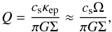 (4)where
κep ≈
Ω is the epicyclic frequency, and cs is the
thermal sound speed. The radial profiles of Q are shown in Fig. 8, for Elias29 for the two cases where an extended disk model is assumed
(Rout ~
300 AU, upper panel) and where a compact disk model is assumed
(Rout ~
15 AU, central panel), and for WL12 (Rout ~ 30 AU,
bottom panel). Even in the case where the extended disk model for Elias 29 is considered,
we see that the disk approaches marginal stability (Q ≈ 1) in the outer disk,
implying that it can also be weakly gravitationally unstable in this case. For the two
other cases considered, where the disk is more compact, the Q parameter formally drops
significantly below unity, indicating that some additional support against self-gravity
needs to be present, for example in the form of turbulent motions generated by the
instability. Gravitational instability is expected to provide turbulent motions at the
sonic level (Lodato & Rice 2004; Cossins et al. 2009) that for both sources would
correspond to vturb on the order of a few
km s-1. Such
turbulent phenomena induced by the disk self-gravity could thus represent an important
source of angular momentum transport to bring Class I objects into the Class II phase.
Additionally, gravitational instabilities are likely to result in strongly time-varying
behavior, such as episodic accretion (Audard et al.
2013) and/or fragmentation into bound objects, such as low-mass stellar
companions or giant planets (Rice et al. 2005).
(4)where
κep ≈
Ω is the epicyclic frequency, and cs is the
thermal sound speed. The radial profiles of Q are shown in Fig. 8, for Elias29 for the two cases where an extended disk model is assumed
(Rout ~
300 AU, upper panel) and where a compact disk model is assumed
(Rout ~
15 AU, central panel), and for WL12 (Rout ~ 30 AU,
bottom panel). Even in the case where the extended disk model for Elias 29 is considered,
we see that the disk approaches marginal stability (Q ≈ 1) in the outer disk,
implying that it can also be weakly gravitationally unstable in this case. For the two
other cases considered, where the disk is more compact, the Q parameter formally drops
significantly below unity, indicating that some additional support against self-gravity
needs to be present, for example in the form of turbulent motions generated by the
instability. Gravitational instability is expected to provide turbulent motions at the
sonic level (Lodato & Rice 2004; Cossins et al. 2009) that for both sources would
correspond to vturb on the order of a few
km s-1. Such
turbulent phenomena induced by the disk self-gravity could thus represent an important
source of angular momentum transport to bring Class I objects into the Class II phase.
Additionally, gravitational instabilities are likely to result in strongly time-varying
behavior, such as episodic accretion (Audard et al.
2013) and/or fragmentation into bound objects, such as low-mass stellar
companions or giant planets (Rice et al. 2005).
7. Summary and conclusion
We present new 3 mm ATCA data of two Class I YSOs in the Ophiucus SFR: Elias29 and WL12. For our analysis we compared them with archival 1.1 mm SMA data (Jørgensen et al. 2009). In the u–v plane the two sources present similar behavior: a constant non-zero emission at the long baselines, which shows the presence of an embedded unresolved disk and an increase of the fluxes at the short u–v distances, related to the presence of an extended envelope. The main results from our analysis are the following.
-
Grain growth in the envelopes. Our observations suggest thatdust grains start to aggregate up to mm sizesalready in the envelope of the two Class I YSOs we have ob-served. This result is in agreement with the evidence of largegrains in the envelope of the Class 0 L1157-mm(Chiang et al. 2012) and withchronological studies of solids found in meteorites (Connellyet al. 2012). The fact that grainscan already grow up to mm-size in the collapsingenvelopes of Class 0 and I is a result that may haveimportant implications on the initial conditions for the models ofdust evolution in protoplanetary disks.
-
Optically thick disks. From our modeling we conclude that the embedded disks in our Class I are probably very compact, with outer radii down to tens of AU, at least for WL12. The existence of such compact disks can suggest that magnetic fields are acting to remove the cloud angular momentum during collapse. The magnetic braking is more efficient during the first stages of collapse (Class 0, or early Class I YSOs) when the envelope is still massive. This may indicate that Elias29 and WL12 are young Class I. If the size of the two sources were confirmed by resolved observations, this would put a strong constraint on models of disk formation. Additionally, such compact disks are expected to be gravitationally unstable, which would result in large turbulent velocities, up to a few km/sec, and in the formation of a spiral structure in the disk that might be observed through ALMA (Cossins et al. 2010).
Surely future higher resolution observations with the Atacama Large Millimeter/submillimeter Array (ALMA), which has the capability to resolve such compact disks, will be needed to accurately describe the structure of Class I YSOs. Moreover, a larger sample of Class I sources, easily obtainable with ALMA’s high sensitivity, would be essential in order to understand how universal our results are.
Online material
Appendix A: Error estimate of the approximate dust opacity spectral index
In the optically thin limit and the Rayleigh-Jeans regime, the dust opacity spectral
index β can
be approximated using the flux density at two wavelengths. In this appendix, we discuss
the error propagation from the observational uncertainty to the deduced β value as done by Chiang et al. (2012). We take F1 and
F2 to be the flux density at frequencies
ν1 and ν2 and
β can be
expressed as in Eq. (1): 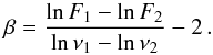 (A.1)We assume that
the variables F1 and F2 are
independent and that σ1 and σ2 are their
standard deviations; propagating the errors we obtain
(A.1)We assume that
the variables F1 and F2 are
independent and that σ1 and σ2 are their
standard deviations; propagating the errors we obtain  (A.2)Calculating the
partial derivative of Eq. (A.1) in both
the variables F1 and F2, we obtain
Combining these two results with Eq. (A.2) we obtain the uncertainty on β:
(A.2)Calculating the
partial derivative of Eq. (A.1) in both
the variables F1 and F2, we obtain
Combining these two results with Eq. (A.2) we obtain the uncertainty on β:
 (A.3)
(A.3)
Appendix B: Estimate of the protostars’ parameters
In order to model the mm emission coming from the disks, the bolometric luminosity Lbol and the effective temperature Teff of the central objects are needed. Once these two parameters are known, then one can obtain the black-body emissions related to the central protostars which are used as the input sources of energy for the computation of the disks dust temperature.
The bolometric luminosities were obtained with Spitzer photometry from the “Cores to Disk” legacy program
(Evans et al. 2009) and are shown in Table 3. On the other hand, in order to obtain Teff some assumptions are needed.
We assume that our two Class I YSOs lie along the stellar birthline, namely the locus in the H-R diagram along which young stars first appear as optically visible objects (Stahler 1983). We adopt the birthline constructed by Palla & Stahler (1990) to obtain Teff given Lbol (Evans et al. 2009) as inputs.
We expect Class I YSOs to have two important contributions from the central protostar: the photospheric stellar luminosity, Lphot (the one just considered), and the accretion luminosity, Lacc. At this stage of evolution Lacc can be comparable with Lphot, while using this simple procedure we are assuming Lacc ≪ Lphot, therefore negligible.
This could in principle lead to some differences in the results, in particular because Lacc tends to enhance the temperature and therefore to change the stellar spectrum. Since we do not have any kind of observation to constrain how much the accretion contributes to the total stellar luminosity, we only assume a photospheric contribution. This could lead to underestimating the temperature in the internal regions of the disk-envelope structure, and thus to overestimating the total dust mass. However, we do not expect this effect to be crucial: Natta et al. (2000) show that the average temperatures of disks around stars with very different Teff change only by a factor of two. This means that our errors on the estimation of the dust mass given by the lack of informations on Lacc is only of a factor of two, which is comparable to the uncertainties we have on the dust opacities.
We can anyway check whether our results are reasonable or not, deducing the effective masses of the central objects and comparing it with the masses Ms given by Jørgensen et al. (2009) and Lommen et al. (2008), presented in Table 1.
From Lbol and Teff we obtain
Reff using the standard photosphere
relation as follows:  (B.1)Then, to deduce
Meff, we use the radius vs. mass
relation obtained by Palla & Stahler
(1990) for a spherical protostar accreting at a rate of 10-5 M⊙
yr-1.
(B.1)Then, to deduce
Meff, we use the radius vs. mass
relation obtained by Palla & Stahler
(1990) for a spherical protostar accreting at a rate of 10-5 M⊙
yr-1.
All the effective parameters obtained with the birthline method are summarized in Table 3 together with the measured protostars masses already present in the literature. The effective mass of Elias 29 is compatible with the measured ones.
We define the inner envelope mass as Minn env ≡ Menv(R < 3000 AU), i.e. the mass enclosed in a sphere of radius R = 3000 AU.
Acknowledgments
The authors wish to thank ATNF&CSIRO staff for the support and the hospitality, F. Trotta and F. Testi for their help during the observing session. The authors also thank E. van Dishoeck and the referee, J. Jørgensen, for insightful comments that significantly improved our work. This work was partly supported by the ESO DGDF program and by the Italian Ministero dell’Istruzione, Università e Ricerca through the grant Progetti Premiali 2012- iALMA.
References
- Allen, A., Li, Z.-Y., & Shu, F. H. 2003, ApJ, 599, 363 [NASA ADS] [CrossRef] [Google Scholar]
- André, P., & Montmerle, T. 1994, ApJ, 420, 837 [NASA ADS] [CrossRef] [Google Scholar]
- André, P., Ward-Thompson, D., & Barsony, M. 1993, ApJ, 406, 122 [NASA ADS] [CrossRef] [Google Scholar]
- Audard, M., Abraham, P., Dunham, M. M., et al. 2013, PPVI Review [Google Scholar]
- Banzatti, A., Testi, L., Isella, A., et al. 2011, A&A, 525, A12 [NASA ADS] [CrossRef] [EDP Sciences] [Google Scholar]
- Beckwith, S. V. W., & Sargent, A. I. 1991, ApJ, 381, 250 [NASA ADS] [CrossRef] [Google Scholar]
- Beckwith, S. V. W., Henning, T., & Nakagawa, Y. 2000, in Protostars and Planets IV, eds. V., Mannings, A.P., Boss, & S. S., Russell (Tucson: University of Arizona Press), 533 [Google Scholar]
- Bergin, E. A., & Tafalla, M. 2007, ARA&A, 45, 339 [NASA ADS] [CrossRef] [Google Scholar]
- Birnstiel, T., Ormel, C. W., & Dullemond, C. P. 2011, A&A, 525, A11 [NASA ADS] [CrossRef] [EDP Sciences] [Google Scholar]
- Butner, H. M., Natta, A., & Evans, N. J., II 1994, ApJ, 420, 326 [NASA ADS] [CrossRef] [Google Scholar]
- Chiang, E. I., & Goldreich, P. 1997, ApJ, 490, 368 [NASA ADS] [CrossRef] [Google Scholar]
- Chiang, H.-F., Looney, L. W., & Tobin, J. J. 2012, ApJ, 756, 168 [NASA ADS] [CrossRef] [Google Scholar]
- Connelly, J. N., Bizzarro, M., Krot, A. N., et al. 2012, Science, 338, 651 [NASA ADS] [CrossRef] [Google Scholar]
- Cossins, P., Lodato, G., & Clarke, C. J. 2009, MNRAS, 393, 1157 [Google Scholar]
- Cossins, P., Lodato, G., & Testi, L. 2010, MNRAS, 407, 181 [NASA ADS] [CrossRef] [Google Scholar]
- Crapsi, A., van Dishoeck, E. F., Hogerheijde, M. R., Pontoppidan, K. M., & Dullemond, C. P. 2008, A&A, 486, 245 [NASA ADS] [CrossRef] [EDP Sciences] [Google Scholar]
- Dapp, W. B., & Basu, S. 2010, A&A, 521, L56 [NASA ADS] [CrossRef] [EDP Sciences] [Google Scholar]
- Dapp, W. B., Basu, S., & Kunz, M. W. 2012, A&A, 541, A35 [NASA ADS] [CrossRef] [EDP Sciences] [Google Scholar]
- de Geus, E. J., de Zeeuw, P. T., & Lub, J. 1989, A&A, 216, 44 [NASA ADS] [Google Scholar]
- Draine, B. T. 2006, ApJ, 636, 1114 [NASA ADS] [CrossRef] [Google Scholar]
- Dullemond, C. P., & Dominik, C. 2004, A&A, 417, 159 [NASA ADS] [CrossRef] [EDP Sciences] [Google Scholar]
- Dullemond, C. P., Dominik, C., & Natta, A. 2001, ApJ, 560, 957 [NASA ADS] [CrossRef] [Google Scholar]
- Dzib, S. A., Loinard, L., Mioduszewski, A. J., et al. 2013, ApJ, 775, 63 [NASA ADS] [CrossRef] [Google Scholar]
- Evans, N. J., Dunham, M. M., Jørgensen, J. K., et al. 2009, VizieR Online Data Catalog: J/ApJS/181/321 [Google Scholar]
- Foster, J. B., Mandel, K. S., Pineda, J. E., et al. 2013, MNRAS, 428, 1606 [NASA ADS] [CrossRef] [Google Scholar]
- Hennebelle, P., & Ciardi, A. 2009, A&A, 506, L29 [NASA ADS] [CrossRef] [EDP Sciences] [Google Scholar]
- Hennebelle, P., & Fromang, S. 2008, A&A, 477, 9 [NASA ADS] [CrossRef] [EDP Sciences] [Google Scholar]
- Hogerheijde, M. R., van Dishoeck, E. F., Salverda, J. M., & Blake, G. A. 1999, ApJ, 513, 350 [NASA ADS] [CrossRef] [PubMed] [Google Scholar]
- Hull, C. L. H., Plambeck, R. L., Bolatto, A. D., et al. 2013, ApJ, 768, 159 [NASA ADS] [CrossRef] [Google Scholar]
- Johnstone, D., Di Francesco, J., & Kirk, H. 2004, ApJ, 611, L45 [Google Scholar]
- Joos, M., Hennebelle, P., & Ciardi, A. 2012, A&A, 543, A128 [NASA ADS] [CrossRef] [EDP Sciences] [Google Scholar]
- Jørgensen, J. K., Hogerheijde, M. R., van Dishoeck, E. F., Blake, G. A., & Schöier, F. L. 2004, A&A, 413, 993 [NASA ADS] [CrossRef] [EDP Sciences] [Google Scholar]
- Jørgensen, J. K., Bourke, T. L., Myers, P. C., et al. 2007, ApJ, 659, 479 [NASA ADS] [CrossRef] [Google Scholar]
- Jørgensen, J. K., van Dishoeck, E. F., Visser, R., et al. 2009, A&A, 507, 861 [NASA ADS] [CrossRef] [EDP Sciences] [Google Scholar]
- Krasnopolsky, R., Li, Z.-Y., & Shang, H. 2010, ApJ, 716, 1541 [NASA ADS] [CrossRef] [Google Scholar]
- Krasnopolsky, R., Li, Z.-Y., & Shang, H. 2011, ApJ, 733, 54 [NASA ADS] [CrossRef] [Google Scholar]
- Kwon, W., Looney, L. W., Mundy, L. G., Chiang, H.-F., & Kemball, A. J. 2009, ApJ, 696, 841 [NASA ADS] [CrossRef] [Google Scholar]
- Lada, C. J. 1987, in Proc. Star Forming Regions (Springer Verlag), IAU Symp., 115, 1 [Google Scholar]
- Li, Z.-Y., Krasnopolsky, R., & Shang, H. 2011, ApJ, 738, 180 [NASA ADS] [CrossRef] [Google Scholar]
- Lodato, G., & Rice, W. K. M. 2004, MNRAS, 351, 630 [Google Scholar]
- Lombardi, M., Lada, C. J., & Alves, J. 2008, A&A, 480, 785 [NASA ADS] [CrossRef] [EDP Sciences] [Google Scholar]
- Lommen, D., Jørgensen, J. K., van Dishoeck, E. F., & Crapsi, A. 2008, A&A, 481, 141 [NASA ADS] [CrossRef] [EDP Sciences] [Google Scholar]
- Looney, L. W., Mundy, L. G., & Welch, W. J. 2003, ApJ, 592, 255 [NASA ADS] [CrossRef] [Google Scholar]
- Mathis, J. S., Rumpl, W., & Nordsieck, K. H. 1977, ApJ, 217, 425 [NASA ADS] [CrossRef] [Google Scholar]
- Mellon, R. R., & Li, Z.-Y. 2008, ApJ, 681, 1356 [NASA ADS] [CrossRef] [Google Scholar]
- Mezger, P. G. 1970, in Proc. The Spiral Structure of our Galaxy (Springer Verlag), IAU Symp. 38, 107 [Google Scholar]
- Miyake, K., & Nakagawa, Y. 1993, 106, 20 [Google Scholar]
- Mohanty, S., Greaves, J., Mortlock, D., et al. 2013, ApJ, 773, 168 [NASA ADS] [CrossRef] [Google Scholar]
- Natta, A., & Testi, L. 2004, Star Formation in the Interstellar Medium: In Honor of David Hollenbach, ASP Conf. Proc., 323, 279 [Google Scholar]
- Natta, A., Grinin, V., & Mannings, V. 2000, in Protostars and Planets IV (Tucson: University of Arizona Press), 559 [Google Scholar]
- Natta, A., Testi, L., Neri, R., Shepherd, D. S., & Wilner, D. J. 2004, A&A, 416, 179 [NASA ADS] [CrossRef] [EDP Sciences] [Google Scholar]
- Natta, A., Testi, L., Calvet, N., et al. 2007, in Protostars and Planets V (Tucson: University of Arizona Press), 767 [Google Scholar]
- Ormel, C. W., Paszun, D., Dominik, C., & Tielens, A. G. G. M. 2009, A&A, 502, 845 [NASA ADS] [CrossRef] [EDP Sciences] [Google Scholar]
- Pagani, L., Bacmann, A., Steinacker, J., Stutz, A., & Henning, T. 2011, EAS Pub. Ser., 52, 225 [CrossRef] [EDP Sciences] [Google Scholar]
- Palla, F., & Stahler, S. W. 1990, ApJ, 360, L47 [NASA ADS] [CrossRef] [Google Scholar]
- Panagia, N., & Felli, M. 1975, A&A, 39, 1 [NASA ADS] [Google Scholar]
- Pollack, J. B., Hollenbach, D., Beckwith, S., et al. 1994, ApJ, 421, 615 [NASA ADS] [CrossRef] [Google Scholar]
- Ricci, L., Testi, L., Natta, A., & Brooks, K. J. 2010a, A&A, 521, A66 [NASA ADS] [CrossRef] [EDP Sciences] [Google Scholar]
- Ricci, L., Testi, L., Natta, A., et al. 2010b, A&A, 512, A15 [NASA ADS] [CrossRef] [EDP Sciences] [Google Scholar]
- Ricci, L., Trotta, F., Testi, L., et al. 2012, A&A, 540, A6 [NASA ADS] [CrossRef] [EDP Sciences] [Google Scholar]
- Rice, W. K. M., Lodato, G., & Armitage, P. J. 2005, MNRAS, 364, L56 [NASA ADS] [CrossRef] [Google Scholar]
- Ridge, N. A., Di Francesco, J., Kirk, H., et al. 2006, AJ, 131, 2921 [NASA ADS] [CrossRef] [Google Scholar]
- Sault, R. J., Teuben, P. J., & Wright, M. C. H. 1995, Astronomical Data Analysis Software and Systems IV, ASP Conf. Ser., 77, 433 [NASA ADS] [Google Scholar]
- Spitzer, L. 1978, Physical processes in the interstellar medium (New York: Wiley-Interscience) [Google Scholar]
- Stahler, S. W. 1983, ApJ, 274, 822 [NASA ADS] [CrossRef] [Google Scholar]
- Terebey, S., Shu, F. H., & Cassen, P. 1984, ApJ, 286, 529 [NASA ADS] [CrossRef] [Google Scholar]
- Testi, L., Natta, A., Shepherd, D. S., & Wilner, D. J. 2001, ApJ, 554, 1087 [Google Scholar]
- Testi, L., Natta, A., Shepherd, D. S., & Wilner, D. J. 2003, A&A, 403, 323 [NASA ADS] [CrossRef] [EDP Sciences] [Google Scholar]
- Testi, L., Andrews, S., Birnstiel, T., et al. 2013, PPVI Review [Google Scholar]
- Tobin, J. J., Hartmann, L., Chiang, H.-F., et al. 2013, ApJ, 771, 48 [NASA ADS] [CrossRef] [Google Scholar]
- Ubach, C., Maddison, S. T., Wright, C. M., et al. 2012, MNRAS, 425, 3137 [NASA ADS] [CrossRef] [Google Scholar]
- Ulrich, R. K. 1976, ApJ, 210, 377 [NASA ADS] [CrossRef] [Google Scholar]
- Yıldız, U. A., Kristensen, L. E., van Dishoeck, E. F., et al. 2013, A&A, 556, A89 [NASA ADS] [CrossRef] [EDP Sciences] [Google Scholar]
- Yorke, H. W., & Bodenheimer, P. 1999, ApJ, 525, 330 [NASA ADS] [CrossRef] [Google Scholar]
All Tables
All Figures
|
Fig. 1 Visibility amplitudes expressed in jansky against the u–v distances in kλ.The data points give the amplitudes per bin. The data are binned in annuli according to u–v distance. In the top panels we present the amplitudes of Elias29: in the left panel, the archival 1.1 mm SMA dataset (Jørgensen et al. 2009), and in the right panel the new 3 mm ATCA dataset. In the bottom panels we plot the same for WL12. The histograms give the expected amplitudes for zero signal. The open triangles at zero u–v distance give the zero spacing 1.1 mm fluxes, interpolated between 850 μm and 1.25 mm single-dish fluxes (Lommen et al. 2008; Jørgensen et al. 2009). The orange lines are the best fits of the observed emission, obtained using a combination of a two-layer disk model (Chiang & Goldreich 1997; Dullemond et al. 2001) surrounded by a power-law density envelope. We used the Monte Carlo radiative transport model RADMC-3D (Dullemond & Dominik 2004) to compute the emission from the envelope. The separate contributions given by the disk and the envelope are plotted with the dotted and dashed lines, respectively |
| In the text | |
|
Fig. 2 Elias29 map: detection of the source at 3 mm. The total flux of the source at 3 mm is 10.36 mJy, with a 3σ rms of 0.18 mJy. |
| In the text | |
|
Fig. 3 WL12 map: detection of the source at 3 mm. The total flux of the source at 3 mm is 17.48 mJy, with a 3σ rms of 0.22 mJy. |
| In the text | |
|
Fig. 4 Visibility amplitudes vs. u–v distances for Elias29 at both 1.1 and 3 mm. The orange line is our best fit of the data, while the blue and green lines represent two models obtained by decreasing and increasing the envelope mass, respectively. We note that these two models also fail to reproduce the single-dish flux at 1.1 mm (Lommen et al. 2008; Jørgensen et al. 2009), shown by the open triangle. |
| In the text | |
|
Fig. 5 Visibility amplitudes vs. u–v distances for WL12 at both 1.1 and 3 mm. The orange line is our best fit of the data, while the blue and green lines represent two models obtained by decreasing and increasing the envelope mass, respectively. We note that these two models also fail to reproduce the single-dish flux at 1.1 mm (Lommen et al. 2008; Jørgensen et al. 2009), shown by the open triangle. |
| In the text | |
|
Fig. 6 Visibility amplitudes vs. u–v distances for Elias29 at both 1.1 and 3 mm. The orange line is our best fit of the data, obtained with a 2 M⊙ envelope, where grains have already grown up to mm size. The green line represents a model obtained with a 1.1 M⊙ envelope, with grains up to the micrometer size, in order to reproduce the 1.1 mm observations. It fails, however, to reproduce the 3 mm data. This shows that only the presence of already grown grains can give the dust an opacity able to reproduce the dual-frequency observations. |
| In the text | |
|
Fig. 7 Millimeter flux density vs. spectral index for disk models for Elias29 (top panel) and WL12 (bottom panel). The black dots show our ATCA data. Each line represents the prediction of disk models with the same disk outer radius and dust opacity spectral index β, but increasing disk mass from left to right. For Elias29 the observed flux and spectral index are consistent with both a small (R ~ 15 AU) optically thick disk, in which case we cannot constrain the dust properties, or a relatively large (R ~ 50–200 AU) optically thin disk populated with cm-sized pebbles. For WL12 the match between the observed data and the models suggests a very small and optically thick disk with a 30 AU radius. It is not possible to determine whether the grains are in the μm- , mm- or cm-sized regime . |
| In the text | |
|
Fig. 8 Radial profile of the stability parameter Q. For Elias29 in the upper panel an extended disk model is assumed (Rout = 300 AU), while in the central panel a compact disk model is assumed (Rout = 15 AU). In the first case, in the outer regions of the disk Q approaches unity, showing marginal stability. In the second case, the value of Q drops below unity, showing the presence of strong gravitational instability. In the bottom panel a compact disk model is assumed (Rout = 30 AU) for WL12. In this case Q also assumes very low values, showing that prominent gravitational instability is present. |
| In the text | |
Current usage metrics show cumulative count of Article Views (full-text article views including HTML views, PDF and ePub downloads, according to the available data) and Abstracts Views on Vision4Press platform.
Data correspond to usage on the plateform after 2015. The current usage metrics is available 48-96 hours after online publication and is updated daily on week days.
Initial download of the metrics may take a while.