| Issue |
A&A
Volume 553, May 2013
|
|
|---|---|---|
| Article Number | A129 | |
| Number of page(s) | 15 | |
| Section | The Sun | |
| DOI | https://doi.org/10.1051/0004-6361/201220804 | |
| Published online | 28 May 2013 | |
Particle scattering in turbulent plasmas with amplified wave modes⋆
1 Lehrstuhl für Astronomie, Universität Würzburg, Emil-Fischer-Straße 31, 97074 Würzburg, Germany
e-mail: This email address is being protected from spambots. You need JavaScript enabled to view it.
2 Centre for Space Research, North-West University, 2520 Potchefstroom, South Africa
3 Department of Physics and Astronomy, University of Turku, 20014 Turun yliopisto, Finland
4 Department of Physics, PO Box 64, University of Helsinki, 00014 Helsinki, Finland
5 Jeremiah Horrocks Institute, University of Central Lancashire, PR1 2HE, Preston, UK
Received: 28 November 2012
Accepted: 6 March 2013
Abstract
High-energy particles stream during coronal mass ejections or flares through the plasma of the solar wind. This causes instabilities, which lead to wave growth at specific resonant wave numbers, especially within shock regions. These amplified wave modes influence the turbulent scattering process significantly. In this paper, results of particle transport and scattering in turbulent plasmas with excited wave modes are presented. The method used is a hybrid simulation code, which treats the heliospheric turbulence by an incompressible magnetohydrodynamic approach separately from a kinetic particle description. Furthermore, a semi-analytical model using quasilinear theory (QLT) is compared to the numerical results. This paper aims at a more fundamental understanding and interpretation of the pitch-angle scattering coefficients. Our calculations show a good agreement of particle simulations and the QLT for broad-band turbulent spectra; for higher turbulence levels and particle beam driven plasmas, the QLT approximation gets worse. Especially the resonance gap at μ = 0 poses a well-known problem for QLT for steep turbulence spectra, whereas test-particle computations show no problems for the particles to scatter across this region. The reason is that the sharp resonant wave-particle interactions in QLT are an oversimplification of the broader resonances in test-particle calculations, which result from nonlinear effects not included in the QLT. We emphasise the importance of these results for both numerical simulations and analytical particle transport approaches, especially the validity of the QLT.
Key words: Sun: particle emission / magnetohydrodynamics (MHD) / Sun: coronal mass ejections (CMEs) / turbulence / acceleration of particles
Appendices A–D are available in electronic form at http://www.aanda.org
© ESO, 2013
1. Introduction
Coronal mass ejections (CME) are believed to be an important source of solar energetic particles (SEP). The acceleration mechanism taking place is the diffusive shock acceleration process (Reames 1999). One cornerstone in the theory behind this mechanism is understanding particle scattering of SEP in the background plasma. The general approach used for this purpose is the quasilinear theory (QLT) (Jokipii 1966).
The CME may be represented as a system of a thermal plasma with a turbulent energy spectrum and a nonthermal proton and electron component. These constituents are interacting with each other in a nonlinear way. In order to understand this system, it is necessary to model wave excitation by particle beams, turbulent energy transfer, and the transport of high-energy particles. Models have been developed by, e.g. Vainio & Laitinen (2007) and Ng & Reames (2008). While these models are capable of describing the interaction of particles and waves, the details of the specific processes are implemented in a simple way, basically relying on QLT or its simple extensions as the correct description of particle scattering and ignoring oblique or perpendicular wave modes completely. Lange & Spanier (2012) did numerical simulations of the turbulent cascading process of energy injected via proton beams. The basic concept of this paper is to take first steps towards a consistent description of particle transport within these plasma configurations and investigate how well the QLT describes scattering in such turbulence.
The general problem in the derivation of transport coefficients is a gap between theoretical and numerical approaches. Numerical simulations have used artificial turbulence spectra (Qin et al. 2002), while analytical calculations use any possible spectrum. However, the applicability of these calculations is unclear. This work combines the previous turbulence simulations by Lange & Spanier (2012) with a particle tracking algorithm derived from Spanier & Wisniewski (2011). The results are compared with QLT calculations using an identical input spectrum.
This approach allows a comparison of QLT and numerical simulations. The latter are assumed to be valid for a wide range of turbulent spectra and particle energies. Therefore, a determination of the validity of QLT is possible. Novel visualization and comparison methods are used to probe nonlinear and time-dependent scattering processes. Thus, a more fundamental understanding of the scattering process is achieved.
2. Theory
2.1. Numerical model
The region of the heliosphere we are interested in is within the weak turbulence regime, with magnetic field fluctuations defined as  (1)where ⟨ δB ⟩ = 0 is the mean value of the fluctuations, which leads to ⟨ B ⟩ = B0. In that sense, weak turbulence is connected to small fluctuation amplitudes compared to the magnetic background field B0. In terms of wave turbulence, this means that the linear Alfvén wave timescale is shorter than the intrinsically nonlinear time. It is observed that the solar wind magnetic fluctuations decrease as δB2 ∝ r-3, while the background field decreases as
  (Bavassano et al. 1982; Bruno & Carbone 2005). Consequently the δB/B0 ratio within the heliosphere is increasing with distance from the Sun (Hollweg et al. 2010).
The magnetic background field B0 is defined towards the z-direction within our simulations and hence is also denoted as B0ez. The parallel direction is, therefore, defined as the z-direction and the x- and y-direction are the perpendicular directions. For symmetry reasons, there will be no further distinction between the two perpendicular directions, and all plots show values averaged over the azimuthal angle in cylindrical coordinates of the x–y plane.
High Reynolds numbers in combination with massive energy injection, as seen in, e.g. the solar wind, are strong indicators of a highly turbulent state. This means that most parts of the heliosphere are dominated by turbulent evolution and consequently energy cascading to smaller spatial scales. In situ measurements of the energy spectrum (Tu et al. 1989) are in agreement with this fact.
To simulate conditions within the turbulent heliospheric plasma with particle transport and scattering, the research group at the University of Würzburg has developed a hybrid simulation code, Gismo. It is divided into two parts, the magnetohydrodynamic (MHD) algorithm Gismo-MHD and the kinetic particle transport simulation tool Gismo-Particles.
Gismo-MHD is an incompressible pseudospectral MHD code that is fully parallelised and capable of efficiently using massive computing clusters. For a more detailed description we refer to Lange & Spanier (2012). A brief overview is presented below. The basis of the simulation software is to solve the following set of incompressible MHD equations: 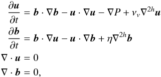 (2)where
  is the normalised magnetic field, u is the fluid velocity, and ϱ is the constant mass density. The dissipative terms due to viscous and Ohmic dissipation are denoted by νv and η. In the following we introduce the parameter ν as a global diffusivity with η = νv ≡ ν. The approach is valid for magnetic Prandtl number of order unity, which is applicable within the regime of Alfvén wave turbulence where an equipartition between magnetic and kinetic energy can be assumed (Bershadskii 2002; Bigot et al. 2008). The artificial increase of the dissipation by the hyperdiffusivity parameter h is often used in spectral methods. The pressure term ∇P fulfils the closure condition for incompressibility (Maron & Goldreich 2001):
  (3)In the incompressible regime of a magnetised plasma, the MHD turbulence consists of only two types of waves, which transport energy along the parallel direction: the so-called pseudo and shear Alfvén waves. The former are the incompressible limit of slow magnetosonic waves and play a minor role within anisotropic turbulence (Maron & Goldreich 2001). The pseudo Alfvén waves polarisation vector is in the plane spanned by the wave vector k and B0. The shear waves are transversal modes with a polarisation vector perpendicular to the k − B0 plane. They are circularly polarised for parallel propagating waves. Both species exhibit the dispersion relation ω2 = (vAk∥)2. We note that the shear mode seems to be dominant because pseudo waves are heavily damped by the Barnes damping process within weakly turbulent regimes (Sridhar & Goldreich 1994). The damping weakens in strong turbulence, but according to Goldreich & Sridhar (1995), the wave generation of pseudo Alfvénic wave modes is only possible via three-wave interactions by two shear wave modes. Barnes damping is important for high-β plasmas. Since this is not fulfilled for the solar corona, the role of pseudo Alfvén waves should not be ignored. However, the solar wind and especially its fast component is strongly dominated by Alfvén waves (Bruno & Carbone 2005; Howes et al. 2012) and therefore incompressible MHD is well applicable.
Because of this model, a suitable description of the system is achieved by the use of Alfvénic waves moving either forwards or backwards. Therefore the Elsässer variables (Elsässer 1950) are introduced:  (4)Applying this definition to Eqs. (2) and transformation to the Fourier space yields
 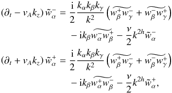 (5)where the tilde-notation represents quantities in the Fourier space. This is the final set of equations which is iterated by Gismo-MHD.
Obviously, the nonlinearities of Eqs. (5) that describe the turbulent behaviour of the MHD plasma cannot be solved in Fourier space in a straightforward fashion. Hence the main numerical load is the transfomation between real and wavenumber space for each iterative step. For this purpose we used the P3DFFT algorithm, which is an MPI-parallelised fast Fourier transfomation based on FFTW3 (Pekurovsky 2011).
A basic problem of spectral methods that use discrete Fourier transformation is the aliasing effect. Because of discrete sampling in the wavenumber space, high k-values exhibit errors that depend on the structure of the real space fields. Therefore we used zero padding, which is also referred to as Orszag’s 2/3 rule, i.e. 2/3 of the wavenumbers below the Nyquist frequency have to be truncated to achieve maximum anti-aliasing, hence reducing the Fourier space resolution to 1/3 of the original wavenumber range (Orszag 1971). This process is repeated for each step, immediately before calculating the nonlinearities and, accordingly, calculating the right-hand side (RHS) of the MHD equations. Consequently, the change in the antialiasing-range of one MHD step is physically correct, but not the long-term evolution.
The code Gismo is capable of using different foward-in-time schemes, namely, Euler and Runge-Kutta (RK) second as well as fourth order. All the simulations in this paper have been peformed using RK-4.
The Alfvén wave generation mechanism by SEPs is not investigated in detail here. The driving mechanism assumed for our simulations is the streaming instability. The estimation of the wave growth rate is described in Vainio (2003). The streaming instability is caused by energetic proton scattering off the coronal Alfvén waves. During the the scattering process the particle changes its pitch-angle cosine by Δμ, while its wave-frame energy remains constant. Thus the particles’ energy in the plasma frame is changed by vApΔμ, where p is the wave-frame particle momentum. Accordingly, the Alfvén wave energy in the plasma frame changes due to energy conservation. Another important instability in the solar corona is the electrostatic instability, which is caused by an electron current and streaming ions. Ion acoustic waves would be generated by this process. However, for the growth rate of these modes a sufficiently high ratio Te/Ti ≫ 1 of the electron and ion temperatures is crucial. Observations and simulations in the vicinity of three solar radii indicate temperature ratios of the order of unity (Landi 2007; Jin et al. 2012). In this regime the ion acoustic waves are also efficiently suppressed by Landau damping. For further reading about the streaming instability we refer to Gary (1993).
The numerical tool for the kinetic simulation of charged test particles is Gismo-Particles. Like Gismo-MHD it is fully parallelised and capable of using massive computing clusters. Its core is the calculation of the relativistic Lorentz force ![Mathematical equation: \begin{eqnarray} \frac{\text{d}}{\text{d}t} \; \gamma \, \vec{v} = \frac{q}{m c}\left[ \,c \vec{E}(\vec{x},t) \,+ \, \vec{v} \times \vec{B}(\vec{x},t)\, \right], \label{eq:lorentzforce} \end{eqnarray}](/articles/aa/full_html/2013/05/aa20804-12/aa20804-12-eq38.png) (6)which acts on the particles at position x through the electric E and magnetic fields B of the plasma. The particle velocities are denoted by v, c is the speed of light and γ represents the Lorentz factor. The Gismo-Particles tool is capable of simulating test particles using physical masses and charges of electrons and ions. The test particles do not influence the background plasma, i.e. self-consistent backreactions to the plasma are neglected. A charged particle within a magnetic field will perform a gyromotion with the frequency
(6)which acts on the particles at position x through the electric E and magnetic fields B of the plasma. The particle velocities are denoted by v, c is the speed of light and γ represents the Lorentz factor. The Gismo-Particles tool is capable of simulating test particles using physical masses and charges of electrons and ions. The test particles do not influence the background plasma, i.e. self-consistent backreactions to the plasma are neglected. A charged particle within a magnetic field will perform a gyromotion with the frequency  (7)and the Larmor radius
  (8)A useful numerical approach for solving Eq. (6) for gyrating particles is the implicit scheme of the Borispush. The basic idea was given by Boris (1970), where the iterations of the Lorentz force are separated in two partial steps. First, the particles are accelerated by the electric field within a half time step. Second, the gyromotion of the particles, which is caused by the magnetic field, is calculated. After that, the electric fields acts again for another half time step to complete the iteration. This approach leads to a discretisation of the Lorentz force with the following set of equations:
 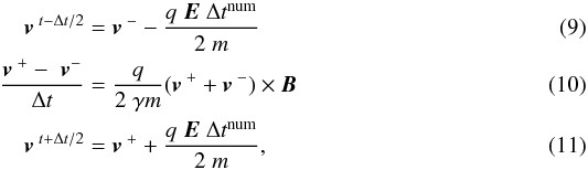 where quantities with Δtnum/2 denote the discrete half-time steps. To solve this set of equations with respect to v+, the following steps were used:
 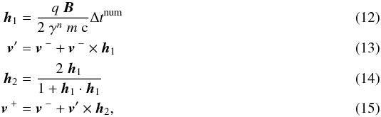 where the auxiliary vectors h were introduced to calculate v+(Birdsall & Langdon 2005). By using these equations, the new velocity and location for each particle are then
 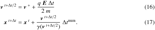 The advantage of the Borispush is the very high numerical stability. The particles are assumed to undergo gyromotions, hence the particle orbits themselves are stable for an arbitrary time discretisation. Even in the limit of Δtnum ≫ Ω-1, the particle orbit is stable but converges to an adiabatic drift motion. The limitation of this method is the correct resolution of the Larmor radius rL. If the timestep chosen is too large, this leads to a big deviation from the analytical rL.
To provide a correct resolution of the gyromotion, Gismo-Particles performs a couple of single-particle gyrations with the used parameters during each start-up phase. The Larmor radius is then measured using a three point-circle approximation. If the deviation to the analytical value is above a given accuracy threshold, the gyrosimulation is performed with a smaller timestep Δtnum. This procedure repeats until the accuracy condition is fulfilled. Specifically, in our simulations an accuracy of the order of |rL − rmeasured| /rL ≈ 10-5 was used. This ensures that in each simulation the time discretisation is chosen correctly. Of course, the discretisation of spatial grid must resolve rL as well. This means that twice the Larmor radius must be much larger than a grid cell and smaller than the whole system length.
Ultrarelativistic particle speeds present limitation to the method of the Borispush. In this case the conservation of energy would be violated, since the ideal ohmic law is not fulfilled anymore. Beyond Lorentz factors of γ ≈ 103, fictitious forces start to act and this approach is no longer applicable (Vay 2008).
Both parts of Gismo are calculated for each step. After iterating the Elsässer MHD fields w±, they are transformed into the physical, electric, and magnetic fields which are transferred to Gismo-Particles. Then the Borispush is performed. Each particle responds to its local fields, which are calculated by an averaging method via three-dimensional splines (Spanier & Wisniewski 2011; Wisniewski et al. 2012). Periodic spatial boundary conditions were used; thus the number of particles remained constant in each simulation.
2.2. Statistical description
The general statistical approach of particle transport by the relativistic Vlasov equation,  (18)describes the development of a particle distribution fT of species T under the influence of the Lorentz force (Schlickeiser 2002). The momentum is denoted by p and the term on the RHS ST is a source term. It is useful to transform this equation into guiding centre coordinates, since we are not interested in the actual position of the gyration, but in the averaged position of the particle. The Vlasov equation then reads
 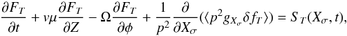 (19)where FT = ⟨ fT ⟩ is the expectation value of fT and Xσ are the guiding centre coordinates with the angle in the perpendicular plane φ and the pitch-angle cosine μ. These coordinates are given by
 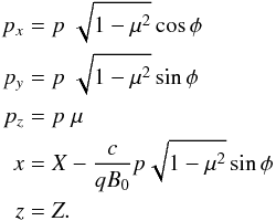 (20)The generalised forces gXσ represent the effects of the electromagnetic fields and are basically the time derivatives of the denoted variables, e.g. gXσ = Ẋσ. This equation is in general analytically unsolvable.
A common approach to describing particle transport analytically is the QLT, which was first suggested by Jokipii (1966) in the context of energetic charged particle transport in turbulent magnetic fields. Its core is the assumption of unperturbed particle orbits. This implies that the fluctuation amplitudes are small, leading to a quasilinear system. The Vlasov equation Eq. (19) would then simplify to 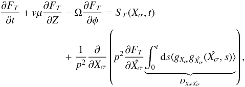 (21)where the method of characteristics was applied and the hat symbol represents quantities along the characteristics (Schlickeiser 2002). This equation is known as the Fokker-Planck equation with the Fokker-Planck coefficients
  . One of the most interesting variables is the pitch-angle diffusion coefficient Dμμ. It describes the pitch-angle scattering of the particle and is consequently connected to the scattering mean free path, which can be evaluated by the observable angle distribution and Monte Carlo simulations (Agueda et al. 2009). Here, scattering means a resonant wave-particle interaction of nth order which fulfils the condition
 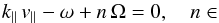 (22)(Schlickeiser 1989), where ω is the wave frequency and k∥ its parallel wavenumber. Ω is again the particle gyrofrequency and v∥ its parallel velocity component. Whether a particle with v∥ interacts resonantly with a wave with k∥ is determined by the polarisation (Kennel & Engelmann 1966). Because our MHD model consists of pseudo and shear Alfvén waves only, certain values of n can be connected to the different types of waves. The Cherenkov resonance, n = 0, is generated only by waves with a compressive magnetic field (δB·B0 ≠ 0), i.e. pseudo Alfvén waves. Purely parallel waves can contribute only to the n = ± 1 resonance, and resonances with | n | > 1 occur only for waves with nonvanishing perpendicular wavenumber, i.e. with oblique Alfvén waves. For a mathematical treatment of the resonant interactions, see Appendix B.
For further reading and a detailed insight of the derivation of Eq. (21) we refer to Schlickeiser (2002). A serious problem of the QLT is the limited applicability. The approximation of small fluctuations only holds for weak turbulent systems, where δB/B0 ≪ 1. This is important for the local field which acts on the invidual particles. For instance, a strong turbulent region would change effectively the direction of the mean magnetic field and consequently the gyromotion of the particles. Hence the assumption of unperturbed orbits would be invalid. Another problem of the QLT is the inadequate description of particles propagating perpendicular to the mean magnetic field, μ ≈ 0. However, regarding Eq. (22) a very small parallel particle velocity will generate a singularity for v∥ → 0. One aspect of this paper will concentrate on the applicability of the QLT to describe solar energetic particle transport.
2.3. The Fokker-Planck coefficient Dμμ
We will now focus on the pitch-angle scattering coefficient in more detail. The basic idea is to compare the simulation results of Gismo with the analytical approach.
Our simulations provide us with all the information of the trajectory and velocity of each individual particle within a turbulent plasma. Particle scattering will be considered here in terms of the pitch-angle cosine  (23)which describes the orientation of the particles’ velocity vector with respect to the local magnetic field. In the approximation of the QLT, there are different ways to calculate Dμμ by using the absolute change of μ during a certain time interval for a single particle. We used the definition
  (24)where the time interval Δt = t − t0 compared to an initial state at t0 is assumed to be large, i.e. the time evolution t has to be sufficient to develop resonant interactions. The necessary time development is discussed in the result section. Instead of using the change of the pitch-angle cosine Δμ = μe − μ0, the definition with the change of the pitch-angle Δα = αe − α0 itself leads to
  (25)which represents the scattering frequency.
For the analytical approach we use the magnetostatic limit for the calculation of Dμμ for pseudo ![Mathematical equation: \begin{eqnarray} D_{\mu\mu,P}&\approx & \frac{2\Omega^{2}(1-\mu^{2})}{B_{0}^{2}} \sum_{n\ne0}\int\, {\rm d}^{3}k\,\pi \delta \left(k_{\parallel}v_{\parallel}+n\Omega\right) \nonumber \\&&\times \left[J_{n}'(v_{\perp}k_{\perp}/\Omega\right]^{2}P_{xx,\rm P}(\vec{k})\label{eq:dmm-sqltP} \end{eqnarray}](/articles/aa/full_html/2013/05/aa20804-12/aa20804-12-eq98.png) (26)and shear Alfvén waves
(26)and shear Alfvén waves ![Mathematical equation: \begin{eqnarray} D_{\mu\mu,A}&= &\frac{2\Omega^{2}(1-\mu^{2})}{B_{0}^{2}} \sum_{n=-\infty}^{\infty}\int\, {\rm d}^{3}k\,\pi\delta\left(k_{\parallel}v_{\parallel}+n\Omega\right) \nonumber \\ &&\times \left[\frac{n\, J_{n}\left(v_{\perp}k_{\perp}/\Omega\right)}{v_{\perp}k_{\perp}/\Omega}\right]^{2}P_{xx,\rm A}(\vec{k}), \label{eq:dmm-sqltA} \end{eqnarray}](/articles/aa/full_html/2013/05/aa20804-12/aa20804-12-eq99.png) (27)where Pxx is the xx-component of the magnetic field fluctuation tensor, which represents the turbulence power spectrum. These equations are based on Schlickeiser (2002) and a more detailed derivation is presented in Appendix B. We note that a proper description of the Cherenkov resonance in Eq. (26) is not possible in this formulation. Using n = 0 yields an undefined mathematical expression. These coefficients were semi-analytically solved with the set of equations given in Appendix C. We note that the approach of the magnetostatic QLT (SQLT) assumes the wave frequency to be small compared to the gyro frequency, ω ≪ Ω.
(27)where Pxx is the xx-component of the magnetic field fluctuation tensor, which represents the turbulence power spectrum. These equations are based on Schlickeiser (2002) and a more detailed derivation is presented in Appendix B. We note that a proper description of the Cherenkov resonance in Eq. (26) is not possible in this formulation. Using n = 0 yields an undefined mathematical expression. These coefficients were semi-analytically solved with the set of equations given in Appendix C. We note that the approach of the magnetostatic QLT (SQLT) assumes the wave frequency to be small compared to the gyro frequency, ω ≪ Ω.
3. Simulation setup
We focus on the environmental conditions in the solar corona at a distance of three solar radii. The magnetic background field in this region is approximately B0 = 0.174G, which yields, assuming a particle density of 105cm-3, an Alfvén speed of vA = 1.2 × 10⁸cms-1(Vainio et al. 2003). This region is of special interest because particle acceleration by CME-driven shocks is strongest there.
The outer length scale of the simulated system is Lscale = 3.4 × 108cm. This value is estimated using the growth rate from Vainio (2003):  (28)with proton cyclotron frequency Ω, proton speed v, the Lorentz factor γ, the proton number density np, as well as μ, the pitch-angle cosine, and f the proton distribution function. As the resonance condition, Eq. (22) is applied, assuming that the particles are streaming along the field.
A remark on the notation: the wavenumber is in general defined as k = (2πj)/L, where j stands for the numerical grid position. For simplicity we used the normalised wavenumbers k′ = kL = (2π·j) throughout.
Parameter setup for the particle simulations.
We generated peaks at  and
and  , which can be excited by streaming protons with energies of Ep ≈ 64MeV and Ep ≈ 7MeV respectively. Using the resonance condition, this leads to a length scale of
 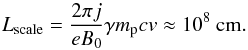 (29)On this scale the magnetic background field is assumed to be homogeneous. The spatial resolution is 2563 gridpoints, resulting in 1283 points in k-space of which | k′ | = 2π [0···42] wave modes are active modes that remain unaffected by (anti)aliasing. The resistivity parameter was set to ν = 1 in numerical units and the hyperdiffusivity coefficient to h = 2.
The turbulence was simulated using an anisotropic driving mechanism. Energy is, therefore, constantly injected into the simulation volume at the first 5 numerical wavenumbers in perpendicular (![Mathematical equation: \hbox{$k'_{\perp}=2 \pi [0\cdots4 ] $}](/articles/aa/full_html/2013/05/aa20804-12/aa20804-12-eq148.png) ) and 15 in parallel direction (
) and 15 in parallel direction (![Mathematical equation: \hbox{$k'_{\parallel}=2 \pi [0\cdots14 ] $}](/articles/aa/full_html/2013/05/aa20804-12/aa20804-12-eq149.png) ). The reference frame is the solar wind frame.
). The reference frame is the solar wind frame.
The anisotropy was chosen for two reasons: first, to mimic the preferential direction of the solar wind, where particles streaming radially away from the Sun form the Parker spiral. Consequently, these particles can deposit their energy in a parallel direction on different scales. This is mainly valid in the vicinity of the Sun, which we are interested in. Second, a slab component of solar wind turbulence is also observed at small scales in the parallel direction. To ensure turbulence evolution up to high parallel wavenumbers, the driving range was extended along the parallel axis. This is necessary because the parallel evolution is much weaker than the perpendicular one (Goldreich & Sridhar 1995, 1997). Even though this is primarily a technical aspect to ensure the extent of the spectrum to higher k∥, it is still in line with observations. An isotropic driver would not yield sufficiently turbulent modes at high k∥.
The turbulence driving is performed by allocating an amplitude with a phase to the Elsässer fields within the Fourier space. The amplitude follows a power-law of | k | -2.5 and is initialised using a normal distribution. The phase was randomly chosen between zero and 2π. These settings are divergence free and Hermitian symmetric. After this initialisation the values were scaled to the desired scenario, which in our case is a δB/B0 ratio of roughly 10-2. We note that both species, pseudo and shear Alfvén waves, are excited by this type of turbulence driving, but as presented by Maron & Goldreich (2001) the pseudo wave evolution is strongly suppressed. In this inertial range energy is injected every 0.03s (10 MHD steps), which leads to a saturated turbulence, an equilibrium between dissipation and injection.
A Gaussian-distributed energy peak with purely parallel wavenumber k = ke∥ was injected within the saturated turbulence. For this purpose, two different wave modes were chosen. To investigate the physics of an SEP-event, a wavenumber of k∥ = 1.5 × 10⁻⁷cm-1 is used. This corresponds to a numerical wavenumber of 2π·8, which is still within the driving range of the turbulence. To represent injection at smaller scales, a peak is set at k∥ = 4.4 × 10⁻⁷cm-1. With  , this wave mode is not in the driving range of the background turbulence. The injection of energy in these modes was done gradually over a specific time interval.
One important aspect of the calculations of Dμμ is the applicability of the QLT. The ratio δB/B0 is, therefore, the limiting parameter (see Sect. 2.2). Consequently, it is of interest to explore peaks at either position under the influence of different magnetic background fields. For this purpose another turbulence simulation was performed which uses the same initial conditions, except for a higher mean field  G and for stability reasons a higher dissipation rate ν = 10cm2hs-1. In the following the smaller field simulation will be denoted by
  . We note that the
  case is an artificial scenario rather than representative of coronal conditions. Peaks in such high magnetic fields represent SEP energies up to 2.65 GeV. In this case the SEPs cannot generate waves by streaming as the relativistic proton intensities are insufficient.
To summarise, these four simulations with excited wave modes at  and , both within turbulent fields governed by a strong and a weak B0, are the starting point for the test particle simulations and the calculations of the scattering coefficient Dμμ.
All of the test particle simulations by Gismo-Particles were performed with 105 protons with an initial uniform distribution in μ and φ and random positions x. This amount has proven to be sufficient in test simulations for good statistics. These initial conditions aim to provide a complete coverage of the phase space in μ for the test particles. Thus, we are not interested in the development of special distribution functions.
A constant absolute value of the momentum was chosen so that particles with a certain parallel velocity component fulfil the resonance condition Eq. (22). Consequently, a resonant value of μ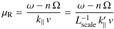 (30)must be within the interval [ − 1;1] for a given particle speed v. Since Eq. (30) is dominated by Ω and hence B0 for particles propagating significantly faster than the Alfvén speed, the particle speed v has to be different for
  and . The parameter setup and the resonant μR for each simulation is summarised in Table 1.
To investigate the particle scattering in different stages of the turbulence evolution, multiple simulations were performed. The most promising match between QLT and the simulation results is expected to be in stages with small δB/B0. According to this, the particle simulations were performed in the driving phase of the peaks as well as in the decaying phase. A simulation at maximum driven peaks would simply lead to random scattering where no reasonable prediction can be made by QLT.
The simulations with the low magnetic background field were also performed with a higher spatial resolution of 5123 grid cells, e.g. 2563 wave modes. For reasons of clarity the results of these simulations are presented and discussed in the Appendix D.
4. Results and discussion
4.1. A toy model for wave-particle resonance
In order to motivate our particle-scattering simulations, we want to present a simple model. Because of the limited applicability of QLT, it is necessary to understand its range of validity. In detail, the δB/B0 ratio and the time development are of utmost importance. Different simplified scenarios are therefore presented below.
We consider a circularly polarised Alfvén wave with k = (0,0,k∥)T. Its magnetic field is described by  (31)in the wave frame where B0 ≫ δB is assumed. The interaction between particles and the wave will then change the particles’ pitch-angles via scatterings. A detailed description of this process as well as a derivation for the time dependency of μ is given in Appendix A. Under the assumption givenby Eq. (31), the expression of the time evolution of μ in Eq. (A.8) will simplify to
 ![Mathematical equation: \begin{eqnarray} \Delta \mu^\pm (t,\psi)& = &\Omega\sqrt{(1-\mu^2)} \, \frac{\delta B}{B_0} \nonumber \\ &&\times\frac{\cos \psi - \cos\left[(\pm k v \mu - \Omega)\Delta t + \psi \right]}{\pm k v \mu - \Omega}, \label{eq:wtr-mu} \end{eqnarray}](/articles/aa/full_html/2013/05/aa20804-12/aa20804-12-eq173.png) (32)when the calculation is performed along the unperturbed orbit, μ = constant. The change in μ is then maximal at the phase
(32)when the calculation is performed along the unperturbed orbit, μ = constant. The change in μ is then maximal at the phase ![Mathematical equation: \begin{eqnarray} \psi^\pm_M = \arctan \left[ \frac{\sin(\pm k v \mu - \Omega)\Delta t}{1-\cos(\pm k v \mu - \Omega)\Delta t} \right] \label{eq:wtr-psi} \end{eqnarray}](/articles/aa/full_html/2013/05/aa20804-12/aa20804-12-eq175.png) (33)and its identical solutions at periods
(33)and its identical solutions at periods  .
.
To study this model, a single linearly polarised Alfvén wave was simulated, propagating undisturbed with vA = 107cm s-1 towards positive z-direction (w+) with a purely parallel wave vector k′ = 2π·(0,0,1)T. It should be noted that the magnetic field given by Eq. (31) does not describe a propagating wave but a static disturbance. Linear polarisation was chosen to cover both resonances at ± μR (respectively both signs in Eq. (32)), because interactions with μ < 0 are caused by left-handed circular polarised waves and μ > 0 by right-handed ones. The wave amplitude was set to δB/B0 = 0.1, where B0 = 4.34 × 10⁻⁴ G. The outer length scale of the simulation cube was set to 108 cm.
In Gismo-Particles, 5 × 10⁵ protons with random μ, φ and position x were initialised. The absolute value of v was set to 2 × 108cm s-1, where particles for n = −1 and n = + 1 are resonant at μR1 = −0.28 and μR2 = + 0.38 according to Eq. (22).
In Fig. 1, we show the pitch-angle change of the simulated particles and the QLT-predicted change as a function of the initial pitch-angle for wave amplitude δB/B = 0.1 after two gyration periods. The simulated particles are represented as a scatter plot, whereas the QLT result for different wave modes are represented by curves. As expected, two maxima develop at the predicted positions μR1 and μR2. The adjoining maxima are caused by particles interacting with the wave nonresonantly, henceforth named nonresonant ballistic interactions. These decrease their amplitudes with increasing time. Also, their positions in μ do not remain constant, like the resonant interactions, because the ballistic maxima become more numerous and move closer to the true resonance. The tilt of the maxima deviates from the prediction of Eq. (32), as clearly shown by comparison with the theoretical curves. Furthermore, the resonances of Eq. (32) are located symmetrically at μr = ± 0.33. This shift can be explained by the choice of the inertial system. The derived equation is within the wave frame. The transformation into the laboratory frame (under the assumption of Galilean transformation) via 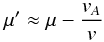 (34)will fit to the observed position in μ. This shift is caused by the magnetostatic approximation, since the difference between Eq. (30) and its magnetostatic version (ω = 0) is exactly the term vA/v. If this ratio is small, as in most of our simulations, the effect is negligible. However, for the simulations with stronger this poses a problem, which will be discussed in the results section.
The tilt cannot be explained by Eq. (32) due to its dependence on the QLT. It stems from the distortion of the orbit by the wave’s δB and consequently, arises by the presentation of Δμ as a function of the initial pitch-angle, μ0. Because of the finite δB/B0-ratio, the assumption of unperturbed orbits, which is the basic approximation in QLT, does not hold anymore. The change of μ should therefore be calculated as an average over the whole trajectory of each particle, which would introduce a nonlinear correction to the theory. A simple solution to correct the tilt is the presentation of Δμ dependent not on the intial μ0, but on the mean value ⟨ μ ⟩ of the initial and the final value of the pitch-angle cosine. We note that the angle of the tilt does not depend on δB/B0, but the scattering amplitude does. Consequently, the tilt is more visible and influences further calculations more as the δB/B0-ratio increases. This visibility is called effective tilt hereafter.
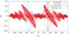 |
Fig. 1 Result of a toy model wave-particle resonance after two gyration periods with a wave amplitude of δB/B0 = 0.1. The pitch-angle scattering is presented in terms of change in Δμ dependent on the particles intial μ0. Each dot represents an individual particle. The theoretical, quasilinear prediction of the maximal change in μ by Eq. (32) deviates clearly from the observed scattering. This type of plot is hereafter denoted as scatter plot. |
In order to prove the explanations given above, we performed a similar simulation with smaller wave amplitude and longer time development. As shown in Fig. 2 the QLT is valid within this scenario. As the scattering amplitude is significantly smaller, the effect of the tilt resulting from using the initial pitch-angle is negligible and the time evolution leads to a clear resonance as the side maxima become smaller. But even under these convenient conditions the deviation from the QLT is still visible.
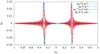 |
Fig. 2 Result of a toy model wave-particle resonance after ten gyration periods with a wave amplitude of δB/B0 = 0.001 . Each dot represents an individual particle scattered from its initial μ0 by Δμ. The prediction by Eq. (32) has been transformed into the lab frame and now describes the observed scattering very well. |
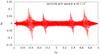 |
Fig. 3 Result of a toy model wave-particle resonance after 50 gyration periods with an oblique wave with an amplitude of δB/B0 = 0.001. As expected, also higher orders of resonances with n = [ − 3, − 2, − 1,1,2] also developed. At this timestep Eq. (32) would again deviate significantly, because only few particles would fulfil the resonance condition, where others are still disturbed by the finite distortion of B0 and thus interact nonresonantly, which produces the finite ballistic background. |
The last case of our toy model uses an oblique wave with k′ = 2π·(0,1,1)T, which was simulated under the same conditions as before. The result in Fig. 3 clearly shows the higher orders of resonance with n = [−3, −2, −1,1,2]. A prediction of Eq. (32) is not applied, since it would not describe the results of the simulation very well for two reasons. First, the assumption that the prediction by QLT becomes better with t → ∞ would not hold because of the finite δB/B0 and hence perturbed orbits. Second, the nonvanishing Bessel functions have to be taken into account and would modify Eq. (32). But although the ballistic maxima become significant in number and generate a nonresonant background scattering, the resonances are clearly visible. Another interesting fact is that the scattering caused by resonance at |n| = 2 exceeds the ones at | n | = 1. This means that in the case of an oblique wave, higher order resonances can become even more important than the fundamental ones. The time development for the purely parallel wave mode at 50 gyration periods showed expectedly only the |n| = 1 resonances (not shown in Fig. 3 for reasons of clarity).
4.2. Results of particle scattering in turbulence with amplified modes
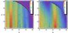 |
Fig. 4 Two-dimensional magnetic energy spectra of both peaks in the simulation with |

We first present selected results from Lange & Spanier (2012), which are the base of our particle simulations. However, we do not discuss the evolution of the peaks in detail, but focus on the stages of the driving and decay of the peaks on which our particle simulations were performed.
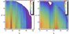 |
Fig. 5 Two-dimensional magnetic energy spectra of both peaks in the simulation with |

In Figs. 4 and 5 we show the situation for the decaying peaks. The timesteps of these figures are the starting points of our particle simulations for the decay stage. We note that the timesteps were chosen to retrieve roughly the same order of magnitude in δB/B0 at the peak positions, which are 10-3. All of the peaks show a strong perpendicular evolution at this stage. Furthermore, higher harmonics of  at positions 16, 24, 32, 40 are present. These harmonics, however, do not interact dominantly with the particles as they have already lost most of their energy compared to the maximum driven stage (not shown here,) as indicated by the logarithmic colour scaling.
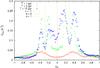 |
Fig. 6 Time evolution of the pitch-angle scattering coefficient Dαα. The setup used is the low |

As shown in the previous section on the toy model, the resonance takes several gyration periods to develop. On the other hand, if the particles are simulated for too long, the interactions with the turbulence will smooth the resonances and lead to unstructured scattering. This is again caused by the finite perturbation of the particle orbits, which are assumed to be negligible for the applicability of QLT. The resonances would not converge to a δ-function as predicted by QLT, but be scattered ballistically at the finite distortions of the fields. We find that a reasonable timescale is between 10 and 30 gyration periods for parameters used in this paper. For weaker turbulence, even results at 50 gyrations might yield a structure, but in most cases the resonances develop clearly in shorter timescales. The pitch-angle scattering coefficient Dαα was calculated for different stages of the evolution. In Fig. 6 we show Dαα for the first simulation setup with  G within the 2563 grid, with the peak position
  at the driven stage. We observe a convergence between 5 and 10 gyration periods. As presented in Table 1, the resonant interaction with the mode is located at μR = 0.29, whereas Fig. 6 shows two maxima at μ = 0.2 and μ = 0.4, which seem to move away from each other during the time development.
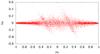 |
Fig. 7 Scatter plot for the low |
The real resonant structure is revealed by the scatter plot in Fig. 7. Indeed, the resonance is centred at the predicted position, but tilted for the same reasons presented with the toy model. The tilt spreads the particles to a wide Δμ range, which results in splitting of the maximum of the pitch-angle diffusion coefficient into two maxima at both sides of the resonant pitch-angle μR = 0.29. This is because the calculation of Dαα in the QLT with Eq. (25) is not dependent on the sign of Δμ. Consequently, the scattering coefficient is mapped due to the square value of Δμ to two different maxima. This also explains the movement of the maxima between five and ten gyration periods in Fig. 6, because Δμ increases with time. The smaller resonance at n = −1, i.e. μR = −0.27, is caused by the different polarisations of the peaked mode. That means resonances with μ < 0 are caused by left-handed circular polarised parts of the peaked mode and μ > 0 by right-handed ones. Furthermore, in the scatter plot the Cherenkov resonance n = 0 is visible. It is hardly observable in the Dαα plot due to the dominant | n | = 1 resonances and their tilt.
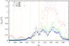 |
Fig. 8 Time evolution of the pitch-angle scattering coefficient Dαα. The setup used is the low |
The test particle simulation with the decay phase of the peaked mode at shows resonant interactions beyond the fundamental resonance. For example, the maximum located near μ = 0.6 in Fig. 8 represents the n = 2 interaction. We note that the tilt in the corresponding scatter plot in Fig. 9 causes again the split of the maximum in Dαα.
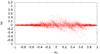 |
Fig. 9 Scatter plot for the low |
As already shown by the toy model, these higher orders are generated by oblique Alfvén waves. Those modes clearly exist in the decay stage of the peaked mode. For example, in Fig. 4 the maximum of the turbulence energy spectrum is shifted from the k∥ axis towards higher perpendicular wave modes. However, within the driven stage of the peak the energy is injected in purely parallel modes, which causes the dominant | n | = 1 resonances. Furthermore, the resonance pattern in Fig. 9 indicates that the left-handed circular polarised parts of the peaked mode decayed faster, which lowers the scattering frequency for particles with μ < 0. While this observation needs further investigation, it seems to be connected to the turbulence evolution, since the wave-particle toymodel does not show this behaviour. Additionally, the magnetic background field plays a role, which is discussed for the results of the other parameter setup below. Again the Cherenkov resonance n = 0 is visible.
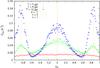 |
Fig. 10 Time evolution of the pitch-angle scattering coefficient Dαα. The setup used is the low |
The results for the particle scattering at the driven peak are presented in Fig. 10. During the driven stage of the peak, the test particles interacted resonantly at | n | = 1 and the predicted pitch-angle μR = 0.86. The effect of the tilt on the resonances is smaller compared to the peak. Consequently, the maxima in the scattering coefficient are not split.
 |
Fig. 11 Scatter plot for the low |
The situation is different for the decay stage. The energy has spread significantly to oblique modes (see Fig. 4, left-hand frame). This leads to stronger scattering and hence a stronger tilt, which is clearly visible in Fig. 11. Even the sharp lines of the maximum change of μ are observed, because several particles were strongly scattered. In this state, Dαα has no clear structure.
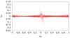 |
Fig. 12 Scatter plots for the high |

The last set of simulations used an increased magnetic background field B0. Thus, the δB/B0 ratio is decreased by an order of magnitude, which is more consistent with the assumptions of the QLT. This claim is supported by Figs. 12 and 13 where each resonance has a reduced effective tilt because of the smaller scattering frequency and represents a dominant structure. We note that the evolution time is roughly twice as long as within the weaker magnetic background field. A strong Cherenkov resonance is observed for the peak. Also both n = | 1 | resonances are visible. The small increase of the scattering rate at 0.53 could be generated by a resonant interaction with the higher harmonic at  , which is also a dominant wave mode in this stage (see Fig. 5, left-hand frame).
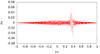 |
Fig. 13 Scatter plots for the high |

For the peak, the fundamental resonance n = 1 is strongest. A higher order of resonance is just slightly visible at μR = 0.70. An indication of the decay of the left-handed modes is the absence of resonant interactions n < 0. These are visible during the driving of the peak, but vanish in the decay stage.
4.3. Comparison between SQLT and particle simulations
In the last section we present results of the SQLT approach and compare them to the particle simulations. For this purpose, the pitch-angle scattering coefficient was calculated by using Eqs. (26) and (27) for each spectrum. In contrast to the particle simulations, the calculations via the SQLT approach produce a clear structure in the scattering coefficient, see Fig. 14. That means that the resonances are not broadened by finite time and the effect of the tilt (see the toy model section) does not influence the values of Dαα.
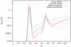 |
Fig. 14 Results for the magnetostatic SQLT approach for the |
As presented in Fig. 14, the magnetostatic calculations of the SQLT reproduce the resonant structures for n = 1,2 very well. However, the resonance gap for small pitch-angle cosine values causes a strong drop-off below | μ | ≲ 0.25. Furthermore, a slab approximation was made by the projection of the total wave energy to the parallel modes, i.e. each wave mode is assumed to be parallel. The slab comparison gives a good approximation of the scattering coefficient, except for the resonant structures caused by the oblique waves (| n | > 1). The scattering caused by the pseudo waves is comparable to the shear waves at the positions of the peaks. For values of μ = [0.35;0.55], the pseudo mode has higher scatter rates than the shear mode, whose coefficient Dαα is bigger elsewhere. In the following, we restrict the presentation to the Dαα sum of both wave modes, e.g. the fourth curve in Fig.14.
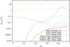 |
Fig. 15 Comparison between SQLT approach and particle simulation of the scattering coefficients Dαα for the low |
As expected, the comparison between SQLT and particle simulation is best for the pure turbulent background case, as long as the Cherenkov resonance is small or for higher values of μ. Because of the resonance gap, it cannot be reproduced by the SQLT approach. However, the particle simulation presents a clear and broad interaction for n = 0, as shown in Fig. 15. Especially for the background and driven stage, the curves increase towards μ = 0, which is caused by the Cherenkov resonance. For a clearer interpretation of Dαα it is again helpful to compare the Dαα curve with the corresponding scatter plot. According to the previous section, the Dαα is not only increased at μ = 0 but also broadened by the tilt of the resonant peak. Nevertheless, the SQLT curve becomes comparable to the particle simulation for μ > 0.6. Because the scattering is concentrated at the purely parallel peak during the driven stage, the scattering coefficient of the particle simulation shows the resonance very well and is also comparable to the SQLT calculation. Even more complicated is the situation for the scattering at the peaked modes in the decay stage. The SQLT curve in Fig. 15 shows the resonance at the predicted position μR = 0.86, whereas the Dαα of the particle simulation seems to have no structure. This is again caused by the visible effect of the tilt at the resonances (see Fig. 11).
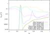 |
Fig. 16 Comparison between SQLT approach and particle simulation of the scattering coefficients Dαα for the low |
Because the effective tilt within the peak simulations is stronger and the resonance pattern for the decay stage is more complex, the particle simulation results for Dαα differ from the SQLT calculations. Nevertheless, the resonances in Fig. 16 are located at the predicted positions.
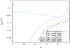 |
Fig. 17 Comparison between SQLT approach and particle simulation of the scattering coefficients Dαα for the high |
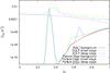 |
Fig. 18 Comparison between SQLT approach and particle simulation of the scattering coefficients Dαα for the high |
The results of the simulation with a higher magnetic background field are presented in Figs. 17 and 18. The qualitative comparison to the SQLT is much better with the smaller δB/B0 ratio. The particle scattering coefficients show clear resonant maxima at the predicted positions. A small shift of the SQLT resonances stems from the magnetostatic assumption, which sets ω in Eq. (30) to zero. This is valid for ω ≪ Ω, which is not fulfilled for this simulation, since ω8 = 177s-1, ω24 = 532s-1 and Ω = 4264s-1. Thus the resonances are slightly shifted towards smaller μR, e.g. the μR = 0.37 for the peak is μR = 0.33 in the magnetostatic limit. Another problem is the resonance gap, which is significantly broader. Consequently, the SQLT curves cannot be compared quantitatively to the particle simulations.
5. Conclusions
To summarise, we firstly presented a simple wave-particle interaction model to achieve a fundamental understanding of the underlying processes and interpretation of numerical simulation results. The effects of tilted and shifted resonances were observed and further compared to QLT predictions. Additionally, the difference between ballistic and resonant interactions could be shown in the context of time development.
Afterwards, we presented three different scenarios:
-
1)
The first scenario used parameters to resemble conditionswithin a heliospheric plasma at three solar radii.
-
2)
To study the influence of the resolution, the first simulation setup was used with a finer grid of 5123 cells (Appendix D).
-
3)
The connection between QLT to a smaller δB/B0 ratio was investigated by an approach using an artificially high B0.
Each scenario was simulated with two different amplified wave modes with peak positions at and 24. Furthermore, two different evolution stages of the peak within the turbulence were investigated, which allows interactions with purely parallel peaked modes to be studied as well as oblique modes because of the peak development towards a perpendicular direction. All of the simulations were performed with 105 protons. Their initial speed was chosen to be in resonance with the peaks. In addition, every turbulence spectrum was used for a magnetostatic QLT approach to calculate the pitch-angle scattering coefficient. We presented resonance patterns with different methods: the scatter plot Δμ (μ0) and the scattering coefficient Dαα (μ0) for both the numerical and semi-analytical quasilinear approach.
Our results show a good agreement between hybrid MHD particle simulations and QLT calculations for the scattering coefficient Dαα for a turbulent broad-band spectrum. The comparison reveals that the SQLT calculations based on the MHD spectrum are missing the Cherenkov resonance (n = 0), which is not covered by the QLT calculations used because quasilinear theory produces a singularity at μ = 0. Furthermore, the resonance gap at small values of | μ | is caused by the power spectrum, which does not have sufficient energy at high wave numbers within the dissipation range of the turbulence. The direct particle simulations, on the other hand, show problems linked to broadened resonances: Because of the finite simulation time, the wave-particle resonance peaks are broadened, which in turn yields a significant scattering background. With increasing simulation time, especially in simulations with higher δB/B0, the resonances did not become narrow but scattering would start to randomise. Consequently, the assumption of δ-shaped resonances does not apply to real particle scattering. Furthermore, the tilt in Δμ, as shown in the scatter plots (e.g. Fig. 7), causes spreading of the resonant peaks over an interval of | μ | for the particle simulations.
Due to the tilt and the broadening of the resonances, the application of the scattering coefficient resulting from Eq. (25) is questionable. The Dαα results are either difficult to interpret or without any reasonable structure. Consequently, the QLT approach does not compare well to the particle simulation results. We point out that in these cases a very nice tool in numerical simulations is the scatter plot. By evaluating the total change of μ versus its initial state μ0, even small resonance patterns become visible. This can be used for correct interpretation of the scattering coefficients. Especially in cases with multiple overlapping resonances (e.g. Fig. 9), the scatter plot yields important information. It should be noted, however, that the analysis of particle-scattering data requires more in-depth research.
A nice comparison between QLT and particle simulations is achieved with smaller δB/B0 ratio of the turbulence and the peaked modes. This is not unexpected, because the assumption of unperturbed orbits is more reasonable. In this case the effective tilt in the scatter plots decreases significantly and Dαα becomes more structured. Unfortunately, the resonance gap in the QLT approach expands in these scenarios, which leads to smaller absolute values of the scattering coefficient. This large gap stems from the used spectrum, where the magnetic background field was increased, leading to less resonant waves.
We conclude that for realistic particle transport, especially around μ ≈ 0, the QLT approach does not yield physical scattering coefficients. This is not unexpected, as it has been discussed in literature already (Shalchi et al. 2004). We are not aware of any self-consistent theory describing the numerical particle results derived from our hybrid simulations. Further investigations are needed to disentangle the different transport processes involved in order to develop a new kind of transport theory. We also note that even our numerical approach has limited validity for high δB/B0 ratios. We will discuss more sophisticated numerical methods for transport analysis in a forthcoming paper.
Online material
Appendix A: Time dependency of the pitch-angle cosine
The interaction of a charged particle with the fluctuation δB of an Alfvén wave forces the particle to leave its gyro orbit. This procedure is referred to pitch-angle scattering. Consequently the change of parallel momentum is connected to this process via  . Then the time derivative of p∥ is given by the Lorentz force
 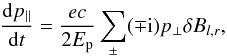 (A.1)where Ep is the energy of the particle, which is assumed to be constant as the scattering is purely elastic. Since the parallel momentum remains constant during an unperturbed gyration, only the perpendicular momentum changes due to the circular movement p⊥ = px ± ipy = p⊥ 0exp [ ∓ i(φ0 − Ωt)]. This leads to a total change of μ for a particle with intial phase φ0 to the magnetic field with
 ![Mathematical equation: \appendix \setcounter{section}{1} \begin{eqnarray} \totdiff{\mu}{t} = \frac{e c}{2 p E_{\rm p}} \sum_\pm(\mp {\rm i}) p_{\perp 0} \exp[\mp {\rm i} (\phi_0-\Omega t)] \delta B_{l,r}(\vec r), \label{eq:mudot} \end{eqnarray}](/articles/aa/full_html/2013/05/aa20804-12/aa20804-12-eq265.png) (A.2)(Lee & Lerche 1974). A similar approach is given by Schlickeiser (2002) using Eq. (19). In this case the solution along the characteristics of the generalised force term
(A.2)(Lee & Lerche 1974). A similar approach is given by Schlickeiser (2002) using Eq. (19). In this case the solution along the characteristics of the generalised force term  is given by Eq. (12.2.4b) Schlickeiser (2002). This result reduces to Eq. (A.2) by using the magnetostatic approximation, which assumes the electric field fluctuations to be negligible, δE = 0. The coordinates used are still Eqs. 20. The fluctuation δB, i.e. of an Alfvén wave as used in the presented case, is given in Fourier space by
 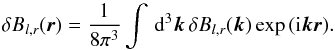 (A.3)The exponential function can be described by the generating Bessel functions Jn
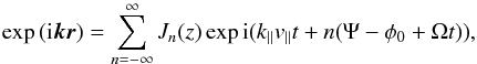 (A.4)where the argument of Jn is
  (A.5)and Ψ = cot-1(kx/ky),
  . The total time derivative of the pitch-angle cosine, separated in parallel and perpendicular interactions, reads then
 ![Mathematical equation: \appendix \setcounter{section}{1} \begin{eqnarray} \bar g_\mu = \totdiff{\mu}{t} &=& \frac{e c}{2 p E_{\rm p}} \sum_\pm(\mp {\rm i}) p_{\perp 0} \exp[\mp {\rm i}\phi_0] \nonumber \\&&\times \frac{1}{8 \pi^3} \int \, \text{d}^3 \vec k \; \delta B_{l,r}(\vec k) \sum_{n=-\infty}^\infty J_n\left(z\right) \nonumber \\&&\times \exp{[ {\rm i} n (\Psi - \phi_0) + {\rm i} t (k_\parallel v_{\parallel} \pm \Omega - n \Omega)]}, \end{eqnarray}](/articles/aa/full_html/2013/05/aa20804-12/aa20804-12-eq274.png) (A.6)For Alfvén waves δB is aligned towards k × ezB0 and consequently δBl,r(k) = δB(k)( ∓ i)exp( ± iΨ). The time integration and the identity
(A.6)For Alfvén waves δB is aligned towards k × ezB0 and consequently δBl,r(k) = δB(k)( ∓ i)exp( ± iΨ). The time integration and the identity  (A.7)(Abramowitz & Stegun 1965) then gives the time dependency of the pitch-angle cosine with
 ![Mathematical equation: \appendix \setcounter{section}{1} \begin{eqnarray} \Delta \mu (t) &= &\mu(t) - \mu_0 = - \frac{e \, c \, p_{\perp 0}}{2 p E_{\rm p} \; 8 \pi^3} \int \, \text{d}^3 \vec k \; \delta B(\vec k) \; \nonumber \\&&\times \sum_{n=-\infty}^\infty [J_{n+1}(z) + J_{n-1}(z)] \; \nonumber \\&&\times \exp{[ {\rm i} n (\Psi - \phi_0)]} \int_0^t \text{d} t' \exp{[ {\rm i} t' (k_\parallel v_{\parallel 0} - n \Omega)]}. \label{eq:mustreuung} \end{eqnarray}](/articles/aa/full_html/2013/05/aa20804-12/aa20804-12-eq278.png) (A.8)The application of a purely parallel propagating wave, as shown in our toy model, will then simplify this equation because z(k⊥ = 0) = 0. Thus, all Bessel functions vanish, except J0(0) = 1. This is the case for n = ± 1. Furthermore, the k integration reduces by the assumption of a single wave
(A.8)The application of a purely parallel propagating wave, as shown in our toy model, will then simplify this equation because z(k⊥ = 0) = 0. Thus, all Bessel functions vanish, except J0(0) = 1. This is the case for n = ± 1. Furthermore, the k integration reduces by the assumption of a single wave  , which leads to the presented form in Sect. 4.1.
Appendix B: Derivation of the pitch-angle diffusion coefficients
In the simulations, the turbulence consists of Alfvén and pseudo Alfvén waves, thus the pitch-angle diffusion coefficient must be calculated separately for the two modes. The two modes are decomposed using the method presented Maron & Goldreich (2001). For the pitch-angle diffusion coefficient for Alfvén waves, Schlickeiser (2002) gives ![Mathematical equation: \appendix \setcounter{section}{2} \begin{eqnarray} D_{\mu\mu,A}&= &\frac{2\Omega^{2}(1-\mu^{2})}{B_{0}^{2}} \sum_{n=-\infty}^{\infty} \int\, {\rm d}^{3}k\,\mathcal{R}\left(\vec{k},\omega\right)\left[1-\frac{\mu\omega}{k_{\parallel}v}\right]^{2} \nonumber \\&&\times \left[\frac{n\, J_{n}\left(v_{\perp}k_{\perp}/\Omega\right)}{v_{\perp}k_{\perp}/\Omega}\right]^{2}P_{xx,\rm A}(\vec{k}), \end{eqnarray}](/articles/aa/full_html/2013/05/aa20804-12/aa20804-12-eq283.png) (B.1)where μ, v and Ω again are the particle’s pitch-angle cosine, speed, and gyrofrequency,
(B.1)where μ, v and Ω again are the particle’s pitch-angle cosine, speed, and gyrofrequency,  , Pxx,A the xx-component of the Alfvén mode turbulence power spectrum tensor, and B0 the background magnetic field. For the resonance function ℛ(k,ω) we assume no damping, which gives the delta function ℛ(k,ω) = π δ(k∥v∥ − ω + nΩ). Thus, in the magnetostatic limit (ω = 0) we have
 ![Mathematical equation: \appendix \setcounter{section}{2} \begin{eqnarray} D_{\mu\mu,\rm A}&= &\frac{2\Omega^{2}(1-\mu^{2})}{B_{0}^{2}} \sum_{n=-\infty}^{\infty}\int\, {\rm d}^{3}k\,\pi\delta\left(k_{\parallel}v_{\parallel}+n\Omega\right) \nonumber \\&&\times \left[\frac{n\, J_{n}\left(v_{\perp}k_{\perp}/\Omega\right)}{v_{\perp}k_{\perp}/\Omega}\right]^{2}P_{xx,\rm A}(\vec{k}). \end{eqnarray}](/articles/aa/full_html/2013/05/aa20804-12/aa20804-12-eq289.png) (B.2)For the magnetosonic waves, Schlickeiser (2002) gives for the fast mode on the cold plasma limit
(B.2)For the magnetosonic waves, Schlickeiser (2002) gives for the fast mode on the cold plasma limit ![Mathematical equation: \appendix \setcounter{section}{2} \begin{eqnarray} D_{\mu\mu,M}&\approx &\frac{2\Omega^{2}(1-\mu^{2})}{B_{0}^{2}} \sum_{n=-\infty}^{\infty} \int\, {\rm d}^{3}k\,\mathcal{R}(\vec{k},\omega) \nonumber \\ &&\times\left[J_{n}'(v_{\perp}k_{\perp}/\Omega\right]^{2}P_{xx,\rm M}(\vec{k}) \end{eqnarray}](/articles/aa/full_html/2013/05/aa20804-12/aa20804-12-eq290.png) (B.3)for high particle velocities, vA ≪ v. As the polarisation of the fast mode on the cold plasma limit is the same as for the pseudo Alfvén wave, it is straightforward to show that the same form also holds for the pseudo Alfvén waves, with the difference in the dispersion relation. However, by using the magnetostatic limit with ω = 0 and again assuming no damping, we get for the resonance function ℛ(k,ω) = πδ(k∥v∥ + Ω), thus giving for the diffusion coefficient
(B.3)for high particle velocities, vA ≪ v. As the polarisation of the fast mode on the cold plasma limit is the same as for the pseudo Alfvén wave, it is straightforward to show that the same form also holds for the pseudo Alfvén waves, with the difference in the dispersion relation. However, by using the magnetostatic limit with ω = 0 and again assuming no damping, we get for the resonance function ℛ(k,ω) = πδ(k∥v∥ + Ω), thus giving for the diffusion coefficient ![Mathematical equation: \appendix \setcounter{section}{2} \begin{eqnarray} D_{\mu\mu,\rm P}&\approx &\frac{2\Omega^{2}(1-\mu^{2})}{B_{0}^{2}} \sum_{n=-\infty}^{\infty}\int\, {\rm d}^{3}k\,\pi\delta\left(k_{\parallel}v_{\parallel}+n\Omega\right) \nonumber \\&&\times \left[J_{n}'(v_{\perp}k_{\perp}/\Omega)\right]^{2}P_{xx,\rm P}(\vec{k}). \end{eqnarray}](/articles/aa/full_html/2013/05/aa20804-12/aa20804-12-eq294.png) (B.4)Unlike for the Alfvén waves, the Cherenkov resonance, n = 0, is nonzero for the pseudo Alfvén waves and has to be considered separately. In this case, the resonance function is
(B.4)Unlike for the Alfvén waves, the Cherenkov resonance, n = 0, is nonzero for the pseudo Alfvén waves and has to be considered separately. In this case, the resonance function is  (B.5)This results in
 ![Mathematical equation: \appendix \setcounter{section}{2} \begin{eqnarray} D_{\mu\mu,P}^{n=0}&= &\frac{2\Omega^{2}(1-\mu^{2})}{B_{0}^{2}} \delta\left(v_{\parallel}\right) \nonumber \\ &&\times \int\, {\rm d}^{3}k\,\frac{\pi}{k_{\parallel}}\left[J_{0}'(v_{\perp}k_{\perp}/\Omega)\right]^{2}P_{xx,\rm P}(\vec{k}), \end{eqnarray}](/articles/aa/full_html/2013/05/aa20804-12/aa20804-12-eq296.png) (B.6)which has a singularity at v∥ = 0, and equals zero elsewhere. Consequently, this term is not used by our model.
(B.6)which has a singularity at v∥ = 0, and equals zero elsewhere. Consequently, this term is not used by our model.
For other terms in the sum over n, we again use the magnetostatic approximation ω = 0, thus giving the resonance condition 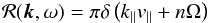 (B.7)and the pitch-angle diffusion coefficient
 ![Mathematical equation: \appendix \setcounter{section}{2} \begin{eqnarray} D_{\mu\mu,P} &\approx & \frac{2\Omega^{2}(1-\mu^{2})}{B_{0}^{2}} \sum_{n\ne0}\int\, {\rm d}^{3}k\,\pi\delta \left(k_{\parallel} v_{\parallel}+n\Omega \right) \nonumber \\ &&\times\left[J_{n}'(v_{\perp}k_{\perp}/\Omega)\right]^{2}P_{xx,\rm P}(\vec{k}). \end{eqnarray}](/articles/aa/full_html/2013/05/aa20804-12/aa20804-12-eq299.png) (B.8)
(B.8)
Appendix C: Discretisation of the pitch-angle diffusion coefficients
For the numerical calculation of the pitch-angle diffusion coefficient, we consider the spectrum to be continuous in parallel direction, but discrete in the perpendicular direction, i.e. Pxx(kx,ky,kz) = Pxx(hΔk,iΔk,kz), with h, i = −M,...,M. In this manner, the integrals over kx and ky can be written as a sum, while the integral over kz is evaluated using the delta function. Then, the diffusion coefficient for the Pseudo-Alfvén waves can be written as ![Mathematical equation: \appendix \setcounter{section}{3} \begin{eqnarray} D_{\mu\mu,P}^{n\neq0} &=&\ \frac{2\pi\Omega^{2}(1-\mu^{2})}{B_{0}^{2}\left|v_{\parallel}\right|} \nonumber \\&&\times \sum_{n=-\infty}^{\infty,n\neq0}\,\sum_{h,i=-M}^{M}\Delta k^{2}\left[J_{n}'(v_{\perp}k_{\perp}/\Omega)\right]^{2} P_{xx,\rm P}(h\Delta k, {\rm i}\Delta k,n\Omega/v_{\parallel}). \end{eqnarray}](/articles/aa/full_html/2013/05/aa20804-12/aa20804-12-eq305.png) (C.1)In this equation, (nΩ)/(μv) represents the parallel wavenumber at which δ(k∥v∥ + nΩ) is nonzero. Consequently, as turbulence data is available only at discrete wavenumbers, we define (nΩ)/(μv) = lΔk. Thus, with l restricted to integer values, we find the values of (v∥ = μv) at which the value of Dμμ can be solved. For a particle with v = Ω/(mΔk), with m ≤ l ≤ M, the pitch-angle is given as μ = m/l. Applying this discretisation, we have
(C.1)In this equation, (nΩ)/(μv) represents the parallel wavenumber at which δ(k∥v∥ + nΩ) is nonzero. Consequently, as turbulence data is available only at discrete wavenumbers, we define (nΩ)/(μv) = lΔk. Thus, with l restricted to integer values, we find the values of (v∥ = μv) at which the value of Dμμ can be solved. For a particle with v = Ω/(mΔk), with m ≤ l ≤ M, the pitch-angle is given as μ = m/l. Applying this discretisation, we have
 (C.2)
(C.2)
and thus ![Mathematical equation: \appendix \setcounter{section}{3} \begin{eqnarray} D_{\mu\mu,P}^{n\neq0}\left(\frac{m}{l}\right) &= & \; 2\pi\Omega\left(1-\frac{m^{2}}{l^{2}}\right)\, l \; \nonumber \\ &&\times \sum_{n=-M/l}^{M/l,\, n\neq0}\:\sum_{h,i=-M}^{M}\left[J_{n}'\left(\frac{1}{m}\sqrt{\left(1-\frac{m^{2}}{l^{2}}\right)\left(h^{2}+i^{2}\right)}\right)\right]^{2} \nonumber \\ &&\times \frac{\Delta k^{3}\: P_{xx,\rm P}\left(h\Delta k, {\rm i}\Delta k,n\, l\,\Delta k\right)}{B_{0}^{2}}\cdot \end{eqnarray}](/articles/aa/full_html/2013/05/aa20804-12/aa20804-12-eq315.png) (C.3)For the Alfvén waves, using the same discretisation, we get
(C.3)For the Alfvén waves, using the same discretisation, we get ![Mathematical equation: \appendix \setcounter{section}{3} \begin{eqnarray} D_{\mu\mu,\rm A}\left(\frac{m}{l}\right)& = & \; 2\pi\Omega\left(1-\frac{m^{2}}{l^{2}}\right)\, l\; \nonumber \\ &&\times\sum_{n=-M/l}^{M/l}\:\sum_{h,i=-M}^{M}\left[\frac{n\, J_{n}\left(\frac{1}{m}\sqrt{\left(1-\frac{m^{2}}{l^{2}}\right)\left(h^{2}+i^{2}\right)}\right)}{\frac{1}{m}\sqrt{\left(1-\frac{m^{2}}{l^{2}}\right)\left(h^{2}+i^{2}\right)}}\right]^{2} \nonumber \\ &&\times\frac{\Delta k^{3}\: P_{xx,\rm A}\left(h\Delta k,i\Delta k,n\, l\,\Delta k\right)}{B_{0}^{2}}\cdot \end{eqnarray}](/articles/aa/full_html/2013/05/aa20804-12/aa20804-12-eq316.png) (C.4)
(C.4)
Appendix D: 5123 results
In this section we present the results of the investigation of the resolution by using a spatial grid of 5123 cells. Again, the MHD simulations were performed, first for the background turbulence, afterward with the peaked modes at and 24. The results are in conformance with the other setups. In particular, we observed the generation of higher harmonic wave modes again.
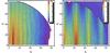 |
Fig. D.1 Two-dimensional magnetic energy spectra of the decay stage for both peaks in the simulation with |
These harmonics are also visible for the peak at within the higher resolved simulation with a 5123 grid. In this simulation setup the number of active modes is eight times greater, which means the antialiasing edge is shifted by a factor two to k′ = 2π·86. Consequently, the higher harmonics at  and 72 are visible. The evolution of the peaks in both simulations is comparable to the 2563 grid simulations. A dominant energy transport towards high perpendicular wavenumbers is observed.
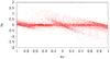 |
Fig. D.2 Scatter plots for the low |

The test particle simulations led to comparable resonance patterns. As presented in Fig. D.2 the resonant interactions at μR = 0,1 and − 0.95 are strongly tilted and a significant amount of particles reach the maximum Δμ, as indicated by the sharp thresholds. The scattering coefficient is in this case again without any structure and hence not shown here. The stronger scattering is primarily caused by the higher wave modes, which are not truncated by the antialiasing anymore and hence contribute to the wave-particle interactions. The test particle simulations were performed for the decay stage of the peaks only because of their huge computational effort.
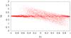 |
Fig. D.3 Scatter plots for the low |
Additionally, an increase of the scattering rate at the peak within the 5123 grid was observed. Consequently, the resonances are not as significant as in the smaller grid. When comparing Fig. 9 and D.3 it is harder to recognize the resonant structures.
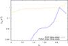 |
Fig. D.4 Comparison between SQLT approach and particle simulation of the scattering coefficients Dαα for the low |
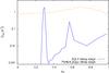 |
Fig. D.5 Comparison between SQLT approach and particle simulation of the scattering coefficients Dαα for the low |
As discussed previously, the 5123 gridsize particle simulation within the decay stage led to strong effectively tilted resonances and consequently a very unstructured Dαα curve. This can be observed in both Figs. D.4 and D.5. Thus, the results differ greatly from those given by SQLT.
Acknowledgments
We acknowledge support from Deutsche Forschungsgemeinschaft through grant SP 1124/3. S.L. additionally acknowledges support from European Framework Program 7 Grant Agreement SEPServer − 262773 and the computing time at Höchstleistungs Rechenzentrum Stuttgart (HLRS). T.L. acknowledges support from the UK Science and Technology Facilities Council (STFC) (grant ST/J001341/1)
References
- Abramowitz, M., & Stegun, I. A. 1965, Handbook of mathematical functions with formulas, graphs, and mathematical tables [Google Scholar]
- Agueda, N., Vainio, R., Lario, D., & Sanahuja, B. 2009, Adv. Space Res., 44, 794 [Google Scholar]
- Bavassano, B., Dobrowolny, M., Fanfoni, G., Mariani, F., & Ness, N. F. 1982, Sol. Phys., 78, 373 [NASA ADS] [CrossRef] [Google Scholar]
- Bershadskii, A. 2002, Phys. Rev. E, 66, 6410 [NASA ADS] [CrossRef] [Google Scholar]
- Bigot, B., Galtier, S., & Politano, H. 2008, A&A, 490, 325 [NASA ADS] [CrossRef] [EDP Sciences] [Google Scholar]
- Birdsall, C. K., & Langdon, A. B. 2005, Plasma physics via computer simulation, 1st edn. (New York: Taylor and Francis) [Google Scholar]
- Boris, J. P. 1970, Proceedings of the Fourth Conference on Numerical Simulation Plasmas, 3 [Google Scholar]
- Bruno, R., & Carbone, V. 2005, Liv. Rev. Sol. Phys., 2, 4 [Google Scholar]
- Elsässer, W. M. 1950, Phys. Rev., 79, 183 [NASA ADS] [CrossRef] [Google Scholar]
- Gary, S. P. 1993, Theory of Space Plasma Microinstabilities [Google Scholar]
- Goldreich, P., & Sridhar, S. 1995, ApJ, 438, 763 [NASA ADS] [CrossRef] [Google Scholar]
- Goldreich, P., & Sridhar, S. 1997, ApJ, 485, 680 [NASA ADS] [CrossRef] [Google Scholar]
- Hollweg, J. V., Cranmer, S. R., & Chandran, B. D. G. 2010, ApJ, 722, 1495 [NASA ADS] [CrossRef] [Google Scholar]
- Howes, G. G., Bale, S. D., Klein, K. G., et al. 2012, ApJ, 753, L19 [NASA ADS] [CrossRef] [Google Scholar]
- Jin, M., Manchester, W. B., van der Holst, B., et al. 2012, ApJ, 745, 6 [NASA ADS] [CrossRef] [Google Scholar]
- Jokipii, J. R. 1966, ApJ, 146, 480 [Google Scholar]
- Kennel, C. F., & Engelmann, F. 1966, Phys. Fluids, 9, 2377 [NASA ADS] [CrossRef] [Google Scholar]
- Landi, E. 2007, ApJ, 663, 1363 [NASA ADS] [CrossRef] [Google Scholar]
- Lange, S., & Spanier, F. 2012, A&A, 546, A51 [NASA ADS] [CrossRef] [EDP Sciences] [Google Scholar]
- Lee, M. A., & Lerche, I. 1974, Rev. Geophys. Space Phys., 12, 671 [NASA ADS] [CrossRef] [Google Scholar]
- Maron, J., & Goldreich, P. 2001, ApJ, 554, 1175 [NASA ADS] [CrossRef] [Google Scholar]
- Ng, C. K., & Reames, D. V. 2008, ApJ, 686, L123 [NASA ADS] [CrossRef] [Google Scholar]
- Orszag, S. A. 1971, Atmosph. Sci., 28, 1074 [NASA ADS] [CrossRef] [Google Scholar]
- Pekurovsky, D. 2011, P3DFFT, Tech. rep., San Diego Supercomputer Center [Google Scholar]
- Qin, G., Matthaeus, W. H., & Bieber, J. W. 2002, ApJ, 578, L117 [NASA ADS] [CrossRef] [Google Scholar]
- Reames, D. V. 1999, Space Sci. Rev., 90, 413 [Google Scholar]
- Schlickeiser, R. 1989, ApJ, 336, 243 [NASA ADS] [CrossRef] [Google Scholar]
- Schlickeiser, R. 2002, Cosmic Ray Astrophysics (Berlin, Heidelberg, New York: Springer) [Google Scholar]
- Shalchi, A., Bieber, J. W., Matthaeus, W. H., & Qin, G. 2004, ApJ, 616, 617 [NASA ADS] [CrossRef] [Google Scholar]
- Spanier, F., & Wisniewski, M. 2011, Astrophys. Space Sci. Trans., 7, 21 [Google Scholar]
- Sridhar, S., & Goldreich, P. 1994, ApJ, 432, 612 [NASA ADS] [CrossRef] [Google Scholar]
- Tu, C.-Y., Marsch, E., & Thieme, K. M. 1989, J. Geophys. Res., 941, 11739 [NASA ADS] [CrossRef] [Google Scholar]
- Vainio, R. 2003, A&A, 406, 735 [NASA ADS] [CrossRef] [EDP Sciences] [Google Scholar]
- Vainio, R., & Laitinen, T. 2007, ApJ, 658, 622 [NASA ADS] [CrossRef] [Google Scholar]
- Vainio, R., Laitinen, T., & Fichtner, H. 2003, A&A, 407, 713 [NASA ADS] [CrossRef] [EDP Sciences] [Google Scholar]
- Vay, J. 2008, Phys. Plasmas, 15, 6701 [Google Scholar]
- Wisniewski, M., Spanier, F., & Kissmann, R. 2012, ApJ, 750, 150 [NASA ADS] [CrossRef] [Google Scholar]
All Tables
All Figures
|
Fig. 1 Result of a toy model wave-particle resonance after two gyration periods with a wave amplitude of δB/B0 = 0.1. The pitch-angle scattering is presented in terms of change in Δμ dependent on the particles intial μ0. Each dot represents an individual particle. The theoretical, quasilinear prediction of the maximal change in μ by Eq. (32) deviates clearly from the observed scattering. This type of plot is hereafter denoted as scatter plot. |
| In the text | |
|
Fig. 2 Result of a toy model wave-particle resonance after ten gyration periods with a wave amplitude of δB/B0 = 0.001 . Each dot represents an individual particle scattered from its initial μ0 by Δμ. The prediction by Eq. (32) has been transformed into the lab frame and now describes the observed scattering very well. |
| In the text | |
|
Fig. 3 Result of a toy model wave-particle resonance after 50 gyration periods with an oblique wave with an amplitude of δB/B0 = 0.001. As expected, also higher orders of resonances with n = [ − 3, − 2, − 1,1,2] also developed. At this timestep Eq. (32) would again deviate significantly, because only few particles would fulfil the resonance condition, where others are still disturbed by the finite distortion of B0 and thus interact nonresonantly, which produces the finite ballistic background. |
| In the text | |
|
Fig. 4 Two-dimensional magnetic energy spectra of both peaks in the simulation with |
| In the text | |
|
Fig. 5 Two-dimensional magnetic energy spectra of both peaks in the simulation with |
| In the text | |
|
Fig. 6 Time evolution of the pitch-angle scattering coefficient Dαα. The setup used is the low |
| In the text | |
|
Fig. 7 Scatter plot for the low |
| In the text | |
|
Fig. 8 Time evolution of the pitch-angle scattering coefficient Dαα. The setup used is the low |
| In the text | |
|
Fig. 9 Scatter plot for the low |
| In the text | |
|
Fig. 10 Time evolution of the pitch-angle scattering coefficient Dαα. The setup used is the low |
| In the text | |
|
Fig. 11 Scatter plot for the low |
| In the text | |
|
Fig. 12 Scatter plots for the high |
| In the text | |
|
Fig. 13 Scatter plots for the high |
| In the text | |
|
Fig. 14 Results for the magnetostatic SQLT approach for the |
| In the text | |
|
Fig. 15 Comparison between SQLT approach and particle simulation of the scattering coefficients Dαα for the low |
| In the text | |
|
Fig. 16 Comparison between SQLT approach and particle simulation of the scattering coefficients Dαα for the low |
| In the text | |
|
Fig. 17 Comparison between SQLT approach and particle simulation of the scattering coefficients Dαα for the high |
| In the text | |
|
Fig. 18 Comparison between SQLT approach and particle simulation of the scattering coefficients Dαα for the high |
| In the text | |
|
Fig. D.1 Two-dimensional magnetic energy spectra of the decay stage for both peaks in the simulation with |
| In the text | |
|
Fig. D.2 Scatter plots for the low |
| In the text | |
|
Fig. D.3 Scatter plots for the low |
| In the text | |
|
Fig. D.4 Comparison between SQLT approach and particle simulation of the scattering coefficients Dαα for the low |
| In the text | |
|
Fig. D.5 Comparison between SQLT approach and particle simulation of the scattering coefficients Dαα for the low |
| In the text | |
Current usage metrics show cumulative count of Article Views (full-text article views including HTML views, PDF and ePub downloads, according to the available data) and Abstracts Views on Vision4Press platform.
Data correspond to usage on the plateform after 2015. The current usage metrics is available 48-96 hours after online publication and is updated daily on week days.
Initial download of the metrics may take a while.