| Issue |
A&A
Volume 551, March 2013
|
|
|---|---|---|
| Article Number | A3 | |
| Number of page(s) | 9 | |
| Section | The Sun | |
| DOI | https://doi.org/10.1051/0004-6361/201220597 | |
| Published online | 07 February 2013 | |
Non-linear force-free magnetic dip models of quiescent prominence fine structures
1 Astronomical Institute, Academy of Sciences of the Czech Republic 25165 Ondřejov Czech Republic
e-mail: This email address is being protected from spambots. You need JavaScript enabled to view it.
2 School of Mathematics and Statistics, University of St. Andrews, St. Andrews, KY16 9SS, UK
3 Max-Planck-Institut für Astrophysik, Karl-Schwarzschild-Str. 1, 85740 Garching bei München, Germany
Received: 19 October 2012
Accepted: 21 December 2012
Abstract
Aims. We use 3D non-linear force-free magnetic field modeling of prominence/filament magnetic fields to develop the first 2D models of individual prominence fine structures based on the 3D configuration of the magnetic field of the whole prominence.
Methods. We use an iterative technique to fill the magnetic dips produced by the 3D modeling with realistic prominence plasma in hydrostatic equilibrium and with a temperature structure that contains the prominence-corona transition region. With this well-defined plasma structure the radiative transfer can be treated in detail in 2D and the resulting synthetic emission can be compared with prominence/filament observations.
Results. Newly developed non-linear force-free magnetic dip models are able to produce synthetic hydrogen Lyman spectra in a qualitative agreement with a range of quiescent prominence observations. Moreover, the plasma structure of these models agrees with the gravity induced prominence fine structure models which have already been shown to produce synthetic spectra in good qualitative agreement with several observed prominences.
Conclusions. We describe in detail the iterative technique which can be used to produce realistic plasma models of prominence fine structures located in prominence magnetic field configurations containing dips, obtained using any kind of magnetic field modeling.
Key words: Sun: filaments, prominences / magnetic fields / radiative transfer / methods: numerical
© ESO, 2013
1. Introduction
Many 2D and 3D magnetic field models have been put forward to explain the global magnetic structure of solar prominences (see Mackay et al. 2010, for a review). The main emphasis of these models is to produce magnetic configurations which contain dips that may support the dense prominence plasma against gravity. These models can be broadly split into two groups, static and dynamic. Static models construct either individual or independent sequences of magnetic configurations where there is no direct correlation or evolution between each extrapolated field (Aulanier & Demoulin 1998; Aulanier et al. 1999, 2000; Mackay et al. 1997, 1999; van Ballegooijen 2004; Dudík et al. 2008). In contrast, dynamic models evolve the magnetic field configurations from one time step to the next (van Ballegooijen & Martens 1989; Galsgaard & Longbottom 1999; Martens & Zwaan 2001; Lionello et al. 2002; DeVore & Antiochos 2000; Mackay & Gaizauskas 2003; Mackay & van Ballegooijen 2005, 2006).
One of the most successful static extrapolation models for explaining the structure and morphology of solar filaments (prominences observed on the solar disk in absorption) is that by Aulanier & Demoulin (1998, see also Aulanier et al. 1999, 2000) where the authors construct either 3D linear force-free fields or 3D linear magnetohydrostatic fields. For a non-linear force-free (NLFF) model see van Ballegooijen (2004). Aulanier & Demoulin (1998) have shown that many observed features of filaments, such as their morphology and barbs may be explained through the location of dips in twisted magnetic flux ropes. A key feature in this work is that barbs are only found to form on either side of the filament when minority polarity magnetic elements lie close to the polarity-inversion line (PIL).
In Dudík et al. (2008) the authors present an observation of a single time snap-shot of a filament that has a gap. Through constructing a linear magnetohydrostatic field they determine that the gap is produced by the filament having a flux rope that is split into two parts. They show that the splitting of the flux rope and therefore the filament is the result of large-scale network fields and not small scale fields.
Mackay & van Ballegooijen (2009) considered how the structure of dips in a filament may vary as a single magnetic bipole is advected towards the main body of the filament. This work, in contrast to previous modeling, considers a time sequence of related magnetic field configurations, rather than a single static extrapolation. It shows how individual magnetic bipoles may perturb the morphology of the filament and result in the break up of the filament into two distinct parts, similar to results of Dudík et al. (2008). In the present paper we utilize results of the 3D NLFF prominence/filament modeling of Mackay & van Ballegooijen (2009) to study the magnetic and plasma structure of individual prominence fine structures.
Local magnetic and plasma structure of prominences has been previously studied by Poland & Anzer (1971) and Heasley & Mihalas (1976) and later by Anzer & Heinzel (1998) and Anzer & Heinzel (1999) who developed 1D magnetic equilibrium models of the Kippenhahn-Schlüter (K-S) type, which were then generalized into 2D by Heinzel & Anzer (2001). Prominence fine-structure models take the form of 2D vertically infinite plasma threads in magnetohydrostatic equilibrium, suspended in 2D magnetic dips. The 2D magnetic equilibrium of K-S type is utilized to create the magnetic and plasma structure locally, but no global equilibrium is considered. The temperature structure of these models is described semi-empirically and includes the prominence-corona transition region (PCTR). By consistently solving 2D multi-level non-LTE (i.e. departures from local thermodynamic equilibrium) radiative transfer in such 2D prominence fine structures, Heinzel & Anzer (2001), Heinzel et al. (2005), and Gunár et al. (2007a) obtained realistic synthetic hydrogen spectrum including Lyman lines, continuum and the Hα line. Such synthetic spectra obtained from a random spatial distribution of 2D threads with realistic values of the plasma parameters are in good agreement with the spectral observations of quiescent prominences. This was demonstrated by Gunár et al. (2007b, 2008, 2010) and more recently by Berlicki et al. (2011) and Gunár et al. (2012). For further details about physical properties of solar prominences, we advise the reader to see classical textbooks such as Tandberg-Hanssen (1995) or comprehensive reviews of Labrosse et al. (2010); Mackay et al. (2010).
In this paper we use the global 3D NLFF prominence/ filament modeling (meaning large-scale modeling of the whole prominence, not the whole Sun) of Mackay & van Ballegooijen (2009, described in Sect. 2) to prescribe individual magnetic dips. These dips are then filled with realistic prominence plasma by the technique described in Sect. 3. Doing so leads to the first models of individual prominence fine structures based on global 3D magnetic field modeling. By computing the radiative transfer in these structures we obtain the synthetic hydrogen spectra. Results are given in Sect. 4. Section 5 presents a validation of the developed technique for filling the NLFF dips and Sect. 6 provides our discussion and conclusions.
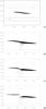 |
Fig. 1 a) Initial condition of a linear force-free field for α = −2.93 × 10⁻⁸ m-1 where dips in the field lines (thick black lines) are plotted to one PSH and viewed from above. The solid/dashed black contours denote positive/negative values of Bz at levels of ± 70, ± 50, ± 1 Gauss. Physical dimensions are given in Mm. In panels b) to d) a close up view of the area enclosed by the dotted box in the panel a) can be seen after 1000, 2000 and 3000, 60 s long time-steps after the bipole has been inserted. |
2. 3D NLFF magnetic field modeling
Observations of solar filaments and prominences often show highly irregular and evolving morphologies. Irregularities include rapid height changes along the length of the filament, in addition to gaps where no plasma emission or absorption is seen. To consider how such a morphology may arise, Mackay & van Ballegooijen (2009) carried out quasi-static 3D NLFF field simulations, of a magnetic element approaching the main body of a filament.
The basic photospheric distribution of magnetic flux was chosen to be that of a magnetic arcade, but with flux concentrations that are displaced from one-another. The separation of the arcades was chosen to be 120 000 km where one unit in the dimension-less length-scale is chosen to be 60 000 km. This choice is arbitrary but is taken such that the arcades lie four typical supergranular cells apart. The basic photospheric flux distribution can be seen in Fig. 1a where solid and dashed contours represent positive and negative flux, respectively. From the photospheric distribution an initial condition of a linear force-free field is constructed where the value of α was fixed at α = −2.93 × 10⁻⁸ m-1 which is sufficiently large that a dipped magnetic field configuration representing the basic structure of a filament is produced. To detect the presence of magnetic dips in the obtained configuration each grid point within the 3D computational domain is tested. Dips occur when the vertical component of the field satisfies  (1)All grid points which satisfy this criterion are used as the starting points for plotting magnetic field lines. To illustrate in a simplified manner, the portion of the dips that may be visible if prominence plasma would be collated in them, the length of the dips are plotted up to a maximum dip depth of one pressure-scale height (PSH, 300 km if assuming an isothermal plasma with a temperature of 10 000 K) or up to the depth of the lower peak of, in general, asymmetrical dip. Such a simple technique allows comparison of the physical extent of the magnetic dips with what might be seen in Hα. By plotting the field lines and computing the dip depth in this manner, it is assumed that the prominence plasma is located in the magnetic dips without significantly deforming them (force-free dips). It should be noted that in this technique, which is commonly applied in global prominence magnetic field models, no filling factor characterizing the number of fine structures, nor any cross-field plasma structure or fine-structure dimensions are assumed. Rather, each dipped field line is plotted to the extent described above and the number and density of plotted dips is described by the number and density of grid points within the 3D computational domain. However, in the work presented here we do not use this visualization technique.
The initial configuration of the 3D simulation, shown in Fig. 1a, contains a region of dips located above the PIL. The dips are midway between the two flux distributions and form a thin elongated filament structure of length 180 000 km, height 18 000 km and maximum width 6000 km. Within the dipped region there are many dipped field lines lying above and adjacent to one-another. No dips run along the entire extent of the filament.
To consider the effect of a magnetic polarity converging towards the main body of the filament a bipole is inserted into the initial configuration through the technique described in Sect. 2.2.3 of Mackay & van Ballegooijen (2009). The bipole is placed in the positive polarity side of the PIL and is aligned parallel to the overlying arcade as can be seen in Fig. 1b. The ratio of bipole flux (Fb) to arcade flux (Fa) is Fb/Fa = 0.0084, while the ratio of bipole to filament flux (Ff) is Fb/Ff = 2.7. With this orientation the minority polarity for this side of the PIL lies closest to the dips and is then advected towards the main body of the filament by a boundary flow. As the minority polarity is advected towards the main body of the filament, the coronal field is perturbed and evolves through a series of quasi-static NLFF states as described by the magneto-frictional technique of van Ballegooijen et al. (2000) and Mackay & van Ballegooijen (2006).
The effect of the minority polarity of the bipole on the morphology of the filament can be seen in Figs. 1b to d, where in each case a close-up view of the region of the filament shown using plotted dips is seen after (b) 1000, (c) 2000, and (d) 3000, 60 s long time-steps. In each of the plots the advection of the minority polarity of the bipole towards the filament body can be clearly seen, while the dominant polarity remains fixed. As the minority polarity converges towards the filament body it still remains partially connected to the dominant bipole polarity and two stages of evolution occur. The first stage is seen in Figs. 1b and c where the presence of the minority polarity does not significantly affect the main body of the filament. This occurs when the minority polarity is still a significant distance away from the filament. Initially the effect of the bipole insertion is to produce a series of new dips within the coronal volume between the minority polarity and the filament dips. The dips branch out to the right and produce a structure that resembles the right bearing barbs of a dextral filament (Aulanier & Demoulin 1998).
As the minority polarity continues to approach the filament’s main body, the second phase of evolution starts (Fig. 1d). In this phase the barbs begin to fully align with the filament’s main body, but the body now breaks into two separate parts and the filament looses its symmetry. The gaps at the center of the body are the result of the absence of dips, not an absence of plotted field lines. The left side of the filament gets thinner and is displaced towards larger y-values, while the right hand side is hardly displaced but becomes much thicker. Therefore the ultimate effect of the minority polarity is to break the filament into two parts. Full details of the evolving magnetic structure can be found in Mackay & van Ballegooijen (2009).
3. Plasma structure of NLFF dips
The plots displayed in Fig. 1 show a purely magnetic representation of a prominence/filament as is often considered by global prominence magnetic field models. In this section, we present a technique that allows us to fill magnetic dips with realistic prominence plasma and thus create the first model of individual prominence fine structures based on global 3D magnetic field modeling. With such a well-defined plasma structure the radiative transfer can be treated in detail and the emerging radiation can be compared with the prominence/filament observations.
3.1. Technique
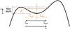 |
Fig. 2 Diagram of an asymmetrical magnetic dip. |
We fill a NLFF magnetic dip iteratively from the dips bottom with plasma in hydrostatic equilibrium. The dip is filled until it either reaches a prescribed column mass, or for the case of an asymmetrical dip, the height of the lower shoulder of the dip is reached. The local geometrical extension L of the left and right part of the dip, is given by the depth of the portion of the dip assumed in each iteration step (see the dip diagram in Fig. 2). L is at each iterative step defined as the distance along the x-direction from the center of the dip towards either the local left or right edge. The temperature variation along the field is defined for the left and right part of the dip separately as  (2)Here ξ represents the geometrical coordinate parallel to x but defined from the center of the local dip towards either its left or right edge. T0 represents the central minimum temperature, Ttr is the transition region temperature and exponent γal describes the temperature gradient along the field.
For the initial estimate of the ionization degree of hydrogen i we use the simple equation ![Mathematical equation: \begin{equation} \label{I_along} i(\xi)=1-(1-i_{\rm c})\left[\frac{T_{\rm tr}-T(\xi)}{T_{\rm tr}-T_{0}}\right]^2 \end{equation}](/articles/aa/full_html/2013/03/aa20597-12/aa20597-12-eq23.png) (3)adapted from Heinzel & Anzer (2001), where ic = 0.3 is the estimated value of the ionization degree at the dip center, as suggested from the results of Anzer & Heinzel (1999). For the mean molecular mass μ of a hydrogen-helium plasma we take
(3)adapted from Heinzel & Anzer (2001), where ic = 0.3 is the estimated value of the ionization degree at the dip center, as suggested from the results of Anzer & Heinzel (1999). For the mean molecular mass μ of a hydrogen-helium plasma we take  (4)where α = 0.1 is the helium-to-hydrogen abundance ratio.
 |
Fig. 3 Schematic representation of the used iterative method. |
To obtain the gas pressure variation along the central field line we define the transition region pressure ptr at both edges of the local dip and then evaluate an integral of the form ![Mathematical equation: \begin{equation} p(z) = p_{\rm tr} \exp\left[\int_{0}^{Z} \frac{\mu(z) \ m_{\rm H} \ g}{k \ T(z)} {\rm d}z\right] \end{equation}](/articles/aa/full_html/2013/03/aa20597-12/aa20597-12-eq29.png) (5)over the depth z-coordinate from both edges towards the bottom of the dip. Here, mH is the mass of the hydrogen atom and g is the gravitational acceleration at the solar surface. Due to the asymmetry of the dip, the value of the central gas pressure pcen at the local total depth Z can, in general, differ between the left and right-part integration, In such case we use the larger of the two values as the true value of the central pressure and perform reversed integration to obtain the pressure variation along the part of the dip which produced the lower central-pressure value. If the pressure obtained at the edge of this part of the dip, resulting from the reversed integration, is larger than the defined ptr we keep the resulting higher value.
(5)over the depth z-coordinate from both edges towards the bottom of the dip. Here, mH is the mass of the hydrogen atom and g is the gravitational acceleration at the solar surface. Due to the asymmetry of the dip, the value of the central gas pressure pcen at the local total depth Z can, in general, differ between the left and right-part integration, In such case we use the larger of the two values as the true value of the central pressure and perform reversed integration to obtain the pressure variation along the part of the dip which produced the lower central-pressure value. If the pressure obtained at the edge of this part of the dip, resulting from the reversed integration, is larger than the defined ptr we keep the resulting higher value.
We then interpolate the pressure variation of the left and right parts of the dip from the z to ξ-coordinate and compute the density as  (6)We then integrate through both parts of the local dip along the ξ-coordinate to obtain the column mass. If the column mass obtained in this iteration step is lower than the required column mass set as an input parameter, we increase the depth of the dip by one depth-step. The scheme of the iterative method is shown in Fig. 3.
To obtain the 2D prominence fine structures we have to define the variation of all quantities, including in the direction across the magnetic field lines (y-direction). Here we assume the cross-field extension of an individual fine structure to be 1000 km, which is consistent with the 2D KS-type models of Heinzel & Anzer (2001). However, observations of filaments in the hydrogen Hα line, such as those of Lin et al. (2005), indicate that the widths of the prominence/filament fine structures may be as small as 100 km. We assume that the shape of the magnetic dip does not change over this distance and thus we use the shape of the central dip at all positions in the cross-field direction.
We define the temperature variation across the field lines in the center of the dip as  (7)where δ = 500 km (total y-extension is 1000 km) and the exponent γac describes the steep temperature gradient across the field. Here we use γac = 60 and a logarithmic scale along the y-axis in order to sufficiently resolve the steep cross-field temperature gradient.
To obtain the gas pressure and density variation across the field lines, we specify the variation of the column-mass in the center of the dip in the cross-field direction as ![Mathematical equation: \begin{equation} \label{M_across} M_{\rm cen}(y) = M_{0} \left[1-\left(\frac{y}{\delta}\right)^{2} \right]\cdot \end{equation}](/articles/aa/full_html/2013/03/aa20597-12/aa20597-12-eq40.png) (8)Thus at the given y-position Mcen(y) is used as the required column mass and Tcen(y) is used as the minimum temperature at the bottom of the dip. The above-described iterative scheme is used to obtain the variation of all quantities along the field line at each y-position.
(8)Thus at the given y-position Mcen(y) is used as the required column mass and Tcen(y) is used as the minimum temperature at the bottom of the dip. The above-described iterative scheme is used to obtain the variation of all quantities along the field line at each y-position.
3.2. Selected NLFF dips
 |
Fig. 4 Scatter plot of length versus depth of all dips contained in 20 simulation snap-shots spanning 4000 time steps with highlighted positions of the two selected dips. |
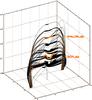 |
Fig. 5 3D visualization of dipped field lines contained in the simulation snap-shot after 2000 time steps (Fig. 1c). Bold lines represent dips and the two selected dips are highlighted in color. Dimensions are given in length-scale units with one unit chosen to be 60 000 km. |
The 3D NLFF modeling of the global prominence magnetic field, such as described in Sect. 2, generates a large number of dipped field lines with a wide range of depths. The majority of these dips, 70% of all dips contained in 20 snap-shots spanning 4000 simulation time steps, have relatively shallow depths below 300 km and only 6% of all dips have depths larger than 1000 km (see Fig. 4). This arises due to the construction of the initial condition (Mackay & van Ballegooijen 2009) which produces only shallow dips due to the absence of any magnetic elements near the PIL or main body of the filament (see Fig. 1a). Deep dips occur as a result of the perturbation of the initial condition as the bipole is emerged and its minority polarity is advected towards the PIL. Because we consider only a single bipole, and it interacts with only a small portion of the length of the filament only a small amount of deep dips are produced. The amount of deep dips could be increased by considering more complex configurations of the photospheric magnetic flux.
We have selected two force-free dips from the NLFF simulation snap-shot after 2000 time steps (Fig. 1c). The first of the selected dips (Deep_dip) represents the minority of dips with depths larger than 1000 km and the second selected dip (Shallow_dip) represents the majority of dips with depths below 300 km. Figure 4 shows the scatter plot of length versus depth of all dips contained in the 20 simulation snap-shots with highlighted positions of the two selected dips. Figure 5 shows a 3D visualization of dipped field lines (bold lines represent dips) contained in the simulation snap-shot after 2000 time steps (Fig. 1c), again with selected dips highlighted. Note, that to translate the dimension-less NLFF modeling into real geometrical distances a length-scale of 60 000 km was used.
The Deep_dip has a depth of nearly 2000 km and to fill it we chose the column-mass along the central field line of M0 = 2 × 10⁻⁴ g cm-2. The along-the-field temperature variation is given by Eq. (2) and the choice of central minimum temperature is T0 = 8000 K, while the transition-region temperature at the edge of a dip is Ttr = 105 K. The exponent γal = 2 describes the temperature gradient along the field. These values (see Table 1) are similar to those used by Gunár et al. (2007b, 2008, 2010) to produce a local 2D KS-type prominence fine-structure model, named Model1 (see Table 2), that is able to reproduce observed hydrogen Lyman spectra. The requirement of M0 = 2 × 10⁻⁴ g cm-2 leads to nearly maximum filling of the Deep_dip with prominence plasma. With a boundary gas pressure, ptr = 0.015 dyn cm-2, the resulting central pressure pcen rises to a relatively high value of 0.13 dyn cm-2 that is comparable with Model1. Figure 6 shows the geometrical dimensions of the Deep_dip with the amount of filling indicated by the horizontal dashed line (and green part of the dipped field line). In addition Fig. 6 shows the temperature and gas pressure variation along the central field line, together with the 2D variation of temperature and gas pressure.
The maximum depth of the Shallow_dip is around 300 km but with the central column mass of M0 = 0.5 × 10⁻⁴ g cm-2 only a half of it is filled with plasma (see Fig. 7). Due to the low depth of the filled dip the gas pressure does not significantly increase from ptr = 0.03 dyn cm-2 and reaches only 0.035 dyn cm-2 in the center. These values (see Table 1) are similar to those of the local 2D KS-type Model2 used by Berlicki et al. (2011) and Gunár et al. (2012) to reproduce the hydrogen Lyman spectra and Hα line observed in the April 26, 2007 prominence (see Table 2).
List of parameters of selected NLFF dips.
List of input parameters of 2D KS-type prominence fine-structure models Model1 (Gunár et al. 2007b) and Model2 (Berlicki et al. 2011).
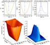 |
Fig. 6 Top left panel shows the geometrical dimensions of the dipped field line of the Deep_dip with amount of filling by prominence plasma indicated by the horizontal dashed line (and green part of the dipped field line). The next two panels show the temperature and gas pressure variation along the central field line. The bottom two panels show the 2D variation of the temperature and the gas pressure. |
4. Synthetic Lyman line profiles
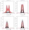 |
Fig. 8 Synthetic profiles produced by the Deep_dip. Lyman-α to Lyman-δ lines are plotted. For each line we plot synthetic profiles obtained at different positions along the x-axis with LOS oriented across the field lines (along the y-axis). Clearly reversed synthetic profiles are highlighted by red lines (only in the online version). |
To determine the synthetic hydrogen spectra originating from the NLFF dips filled with prominence plasma, we have adopted the technique developed by Heinzel & Anzer (2001) for 2D prominence fine-structure thread models. We again assume 2D vertically infinite geometry with all quantities uniform along the vertical axis and varying within the horizontal x-y plane. Such an approach is valid for modeling of prominences observed on the solar limb, as they are often composed of quasi-vertical threads and the dominant incident radiation from the disk penetrates the prominence body along the horizontal plane. Moreover, the shape of the magnetic dips in the global 3D modeling does not vary significantly with height. We solve the 2D multi-level non-LTE (i.e. departures from local thermodynamic equilibrium) radiative transfer problem in the x-y plane using Accelerated Lambda Iteration technique developed in 2D by the Auer & Paletou (1994, see also Paletou 1995), with preconditioned non-LTE statistical equilibrium equations (Rybicki & Hummer 1991, 1992) and assuming a 5-level plus continuum hydrogen atom. The ionization of hydrogen is treated as in Heinzel (1995). We adopt partial redistribution (PRD, Heinzel et al. 1987; Paletou 1995) for Lyman-α and Lyman-β lines. The details of this technique are given in Heinzel & Anzer (2001) and Heinzel et al. (2005).
The radiative transfer computations show that the Deep_dip can produce synthetic spectra containing a large number of profiles with central reversal in lines higher than Lyman-α (which is nearly always reversed). This is caused by the relatively large central gas pressure as a result of sufficient depth of the Deep_dip (nearly 2000 km). Synthetic profiles of Lyman-α to Lyman-δ lines produced by Deep_dip are shown in Fig. 8, where for each spectral line we plot synthetic profiles obtained at different positions along the x-axis with the line of sight (LOS) oriented across the field lines (along the y-axis). On the other hand, the Shallow_dip, which is nearly isobaric due to its low depth, is unable to produce reversed synthetic profiles above Lyman-α (see Fig. 9). Note, that to fill the Shallow_dip we have used M0 = 0.5 × 10⁻⁴ g cm-2, which is comparable to the 2D KS-type Model2. To fill the magnetic dip of the Shallow_dip fully we need central column mass of M0 = 1.0 × 10⁻⁴ g cm-2. However, even such a fully loaded Shallow_dip would only result in a central gas pressure of 0.045 dyn cm-2, which would again lead to non-reversed synthetic Lyman profiles.
For comparison of the synthetic spectra with observed quiescent prominence spectra, we use two sets of observations. The first is that of a prominence observed on May 25, 2005 and contains a large set of spectra from Lyman-α to high members of the Lyman series. Most of the observed Lyman line profiles of all Lyman lines exhibit significant central reversal (see Fig. 10, left half). As was shown by Gunár et al. (2007b) on the profile-to-profile basis and by Gunár et al. (2010) on the statistical bases, Model1 produces synthetic spectra in good agreement with these observations. The second observation is of Apr. 26, 2007 prominence and contains Lyman spectra from Lyman-β to higher Lyman series members (Fig. 10, right half). All observed profiles are non-reversed. This prominence was studied by Berlicki et al. (2011) and Gunár et al. (2012) who showed that models similar to Model2 can produce synthetic Lyman spectra in agreement with this observation.
This comparison shows that when magnetic dips produced by NLFF modeling are realistically filled with prominence plasma they can lead to prominence fine structure models producing synthetic spectra in qualitative agreement with both types of observed Lyman spectra, namely, significantly reversed and also non-reversed Lyman line profiles. However, it is not the purpose of this paper to find NLFF dips that would result in synthetic spectra in quantitative agreement with these observations.
We do not focus in the present work on the Hα line, since to properly compare synthetic Hα profiles with observations, we would have to go beyond the scope of this paper and model a multi-thread structure. This is due to the low Hα optical thickness of individual prominence fine structures. In fact, the maximum value of the Hα optical thickness of the Deep_dip in the direction perpendicular to the magnetic field is 0.67, while for the Shallow_dip it is only 0.13. Correspondingly, the maximum value of the specific intensity of the synthetic Hα line at its center for the Deep_dip is relatively low 1.1 × 10⁻⁶ erg s-1 cm-2 sr-1 Hz-1, while for the Shallow_dip it is very low 0.25 × 10⁻⁶ erg s-1 cm-2 sr-1 Hz-1. Qualitative comparison with the observed Hα values of the Apr. 26, 2007 prominence (Berlicki et al. 2011; Gunár et al. 2012) which has a maximum specific intensity value at the Hα line center above 3.0 × 10⁻⁶ erg s-1 cm-2 sr-1 Hz-1 show that the Deep_dip would require several identical fine structures aligned along the LOS to produce synthetic Hα profiles similar to such observations. In contrast the Shallow_dip would require tens of identical fine structures to produce similar results. However, this is only a preliminary analysis of the synthetic Hα spectra produced by NLFF dips filled with prominence plasma. We will study the Hα spectra in greater detail in our future work.
5. NLFF dips-filling technique verification
The models, described above, of individual prominence fine structures based on global 3D NLFF magnetic field modeling consider only the effect of gravity on the plasma in hydrostatic equilibrium. The gravity effects that would cause a change of the magnetic field structure itself are not considered. In doing so we assume that the dipped field lines are rigid. On the other hand, 2D KS-type models of Heinzel & Anzer (2001, such as Model1 and Model2) are caused entirely by the weight of the prominence mass creating the magnetic dip in initially horizontal field.
To verify the technique for filling of the NLFF magnetic dips by realistic prominence plasma (Sect. 3.1) we apply it on the gravity-induced magnetic dips of the 2D KS-type models, Model1 and Model2. We extract the central dipped field line from these models and fill it with prominence plasma without any additional change to the field-line shape. We use as input parameters the central and boundary temperatures and a column mass identical to Model1 and Model2 (see Table 2). Resulting models, named Adapted_Model1 and Adapted_Model2, are shown in Figs. 11 and 12.
Because the KS-type models describe only the interior of the prominence (including the PCTR) but do not model the surrounding coronal field, the depth of their magnetic dips cannot be directly compared with the depths of NLFF dips (see extreme depth of 8000 km of the Adapted_Model1). Also, the shape of the central dipped field line of the KS-type models, together with the temperature and gas pressure, is determined by the balance of the magnetic and plasma pressure (using an analytical description based on the column-mass coordinate m, see Heinzel & Anzer 2001) and furthermore by the radiation field. The equilibrium between the radiation field and plasma structure of 2D KS-type models is established via iterations of the hydrogen ionization degree developed by Heinzel & Anzer (2003). Thus the temperature profile of the KS-type models cannot be described by an analytical formula and cannot be directly compared with the NLFF models. Note that at this stage we do not utilize ionization degree iterations in the NLFF models, but these can be, and indeed should be, used when NLFF models will be employed for quantitative analyses of observations. Figure 11 shows, plotted by black dashed lines, the temperature and gas pressure profiles of the KS-type Model1. The deviations from the Adapted_Model1 occur in the outer, high temperature, regions where the gas pressure is low. The central pressure obtained by partially filling magnetic-dips of Adapted_Model1 and Adapted_Model2 up to the required column mass (see Figs. 11 and 12) are very similar to those obtained by KS-type models (see Table 2). Also the synthetic spectra produced by Adapted_Model1 and Adapted_Model2 are similar to those obtained by KS-type models Model1 and Model2.
In the NLFF models we have used the exponent γal = 2 to describe the temperature gradient along the magnetic field. This cannot be directly compared with the γ1 from KS-type models (10 for Model1 and 5 for Model2) because the temperature profile in KS-type models is based on the mass coordinate m and in x-coordinate has a sigmoidal shape. However, the value of γal = 2 agrees well with the central part of the temperature profile of KS-type models and differs only in the high temperature part, above approximately 50 000 K. Higher values of the exponent γal will lead to more extended regions of the central minimum temperature part and thus result in nearly identical values of the central gas pressure, but at smaller total depths.
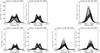 |
Fig. 10 Example of published observed Lyman line profiles obtained by SOHO/SUMER from May 25, 2005 prominence (left half), and Apr. 26, 2007 prominence (right half). Lyman-α to Lyman-δ line profiles are plotted for the first prominence, and Lyman-β to Lyman-δ line profiles are plotted for the second prominence. Each panel contains profiles from all pixels along the SUMER slit that belong to the observed prominence. |
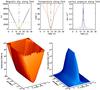 |
Fig. 11 Same as in Fig. 8 but for the Adapted_Model1. In addition, here we plot by black dashed lines, the temperature and gas pressure profiles of the KS-type Model1. |
6. Discussion and conclusions
The NLFF models of individual prominence fine structures, based on global 3D modeling presented in this work do not consider any deformation to the structure of the magnetic dips caused by the weight of the loaded prominence mass. The question now arises as to what extent this force-free field approximation is reasonable. This is true as long as the ratio between the gas pressure and magnetic pressure (plasma β ) is ≪ 1. From the global 3D modeling we can get, by scaling the peak arcade flux at the photosphere to a modest value of 25 G, field strengths in the dipped region of approximately 7 G. Thus we obtain for the Deep_dip a low value of the plasma β = 0.07. This would increase to β = 0.2 in the case of Adapted_Model1 and dip field strength of 7 G but would decrease again to β = 0.1 for a field strength of 10 G. This shows that for typically expected quiescent prominence magnetic field strengths, the shape of the NLFF dips could be changed slightly due to the presence of the plasma, but significant distortions of the field are not expected. Those would arise only in the case of low field strengths of around 3 G combined with higher central pressures. However, care must be taken due to the fact that the NLFF dips are very shallow with small values of the vertical magnetic field component Bz. Therefore, the inclusion of the prominence plasma, even though in the low plasma β regime, could lead to a significant change in the Bz field component and thus to significantly deeper dips. This is, however, beyond the scope of the present paper and it should be considered in future in MHD modeling. We note that the gas pressure can be determined spectroscopically and thus the key question is the strength of the prominence fine-structure magnetic fields. This is a big challenge for future polarization observations.
We have developed a method that allows us to fill NLFF magnetic dips with prominence plasma and thus create realistic models of individual prominence fine structures based on global 3D magnetic field modeling. These models are able to produce synthetic hydrogen spectra (especially Lyman lines) in qualitative agreement with a range of quiescent prominence observations. Moreover, the plasma structure produced in the NLFF models is similar to that of the 2D KS-type models developed by Heinzel & Anzer (2001) and successfully used by Heinzel et al. (2005); Gunár et al. (2007a,b, 2008, 2010, 2011, 2012); Schmieder et al. (2007); Berlicki et al. (2011) to study several problems of the prominence structure and dynamics.
The availability of realistic models of individual prominence fine structures located in global 3D magnetic fields will allow us in future to consistently visualize the whole sets of prominence/filament fine structures with any LOS orientation, either as a prominence in emission above the solar limb, or as dark filament seen in absorption against the solar disk. Such visualizations based solely on the magnetic field structure are currently done in a simplified manner. In particular, the position and dimensions of the magnetic dips in a global 3D simulation is represented by line segments with length corresponding to the portion of the dip filled to a dip depth of one PSH (but see also Heinzel & Anzer 2006). Each dipped field line is plotted and the number and the density of such plotted representations of prominence/filament fine structures is dependent only on the number and density of grid points within the 3D computational domain. Although this simplified method is used as a representation of the Hα line visibility it does not account for any radiative transfer effects. Using such a method, the Deep_dip would be visualized only to a dip depth of one PSH reached at the depth of 400 km (total depth of the Deep_dip is nearly 2000 km), while the Shallow_dip would be visualized entirely. However, the PSH of the Shallow_dip reaches only 0.17 which might suggest that such a dip would not be clearly visible in the Hα line. Thus the current visualization method might lead to an exaggeration of the number of truly observable fine structures, while it underestimates the dimensions of the strongly visible deep dips. In our future work we will concentrate on the use of the synthetic Hα line for visualization of the plasma structure of the global 3D prominence magnetic field modeling. However, the 3D NLFF modeling of Mackay & van Ballegooijen (2009) used in this work contains only a small number of deep magnetic dips with the majority of the dips shallow. This would lead to a simulated prominence with relatively less visible fine structures in the Hα line (although integration through several fine structures would improve the overall visibility) but also such a prominence would exhibit mostly non-reversed Lyman lines above Lyman-α. To obtain reversed Lyman line profiles from a dominant part of the simulated prominence, this would have to contain a much larger portion of deep dips than can be achieved by the current 3D NLFF modeling of Mackay & van Ballegooijen (2009). However, while this modeling contains only a small number of deep dips, it should be noted that the effect of the gravity on the dips has not been considered. Presently it is unclear how gravity will affect the morphology of the dipped field lines, but it could
lead to an enhancement in the number of deep dips. Such an effect is beyond the scope of the present work but we will consider it in the future.
Acknowledgments
S.G. and P.H. acknowledge the support from grant 209/12/0906 of the Grant Agency of the Czech Republic. P.H. acknowledges the support from grant P209/10/1680 of the Grant Agency of the Czech Republic. S.G. and P.H. acknowledge the support from the MPA Garching; U.A. thanks for support from the Ondřejov Observatory. S.G. acknowledges the support from St Andrews University. Work of S.G. and P.H. was supported by the project RVO: 67985815. DHM acknowledges financial support from the STFC and the Leverhulme Trust. In addition research leading to these results has received funding from the European Commission’s Seventh Framework Programme (FP7/2007-2013) under the grant agreement SWIFF (project N° 263340, http://www.swiff.eu). The authors acknowledge support from the International Space Science Institute, Bern, Switzerland to the International Team 174.
References
- Anzer, U., & Heinzel, P. 1998, Sol. Phys., 179, 75 [NASA ADS] [CrossRef] [Google Scholar]
- Anzer, U., & Heinzel, P. 1999, A&A, 349, 974 [NASA ADS] [Google Scholar]
- Auer, L. H., & Paletou, F. 1994, A&A, 285, 675 [NASA ADS] [Google Scholar]
- Aulanier, G., & Demoulin, P. 1998, A&A, 329, 1125 [NASA ADS] [Google Scholar]
- Aulanier, G., Démoulin, P., Mein, N., et al. 1999, A&A, 342, 867 [NASA ADS] [Google Scholar]
- Aulanier, G., Srivastava, N., & Martin, S. F. 2000, ApJ, 543, 447 [NASA ADS] [CrossRef] [Google Scholar]
- Berlicki, A., Gunar, S., Heinzel, P., Schmieder, B., & Schwartz, P. 2011, A&A, 530, A143 [NASA ADS] [CrossRef] [EDP Sciences] [Google Scholar]
- DeVore, C. R., & Antiochos, S. K. 2000, ApJ, 539, 954 [NASA ADS] [CrossRef] [Google Scholar]
- Dudík, J., Aulanier, G., Schmieder, B., Bommier, V., & Roudier, T. 2008, Sol. Phys., 248, 29 [NASA ADS] [CrossRef] [Google Scholar]
- Galsgaard, K., & Longbottom, A. W. 1999, ApJ, 510, 444 [NASA ADS] [CrossRef] [Google Scholar]
- Gunár, S., Heinzel, P., & Anzer, U. 2007a, A&A, 463, 737 [NASA ADS] [CrossRef] [EDP Sciences] [Google Scholar]
- Gunár, S., Heinzel, P., Schmieder, B., Schwartz, P., & Anzer, U. 2007b, A&A, 472, 929 [NASA ADS] [CrossRef] [EDP Sciences] [Google Scholar]
- Gunár, S., Heinzel, P., Anzer, U., & Schmieder, B. 2008, A&A, 490, 307 [NASA ADS] [CrossRef] [EDP Sciences] [Google Scholar]
- Gunár, S., Schwartz, P., Schmieder, B., Heinzel, P., & Anzer, U. 2010, A&A, 514, A43 [NASA ADS] [CrossRef] [EDP Sciences] [Google Scholar]
- Gunár, S., Parenti, S., Anzer, U., Heinzel, P., & Vial, J.-C. 2011, A&A, 535, A122 [NASA ADS] [CrossRef] [EDP Sciences] [Google Scholar]
- Gunár, S., Mein, P., Schmieder, B., Heinzel, P., & Mein, N. 2012, A&A, 543, A93 [NASA ADS] [CrossRef] [EDP Sciences] [Google Scholar]
- Heasley, J. N., & Mihalas, D. 1976, ApJ, 205, 273 [NASA ADS] [CrossRef] [Google Scholar]
- Heinzel, P. 1995, A&A, 299, 563 [NASA ADS] [Google Scholar]
- Heinzel, P., & Anzer, U. 2001, A&A, 375, 1082 [NASA ADS] [CrossRef] [EDP Sciences] [Google Scholar]
- Heinzel, P., & Anzer, U. 2003, in Stellar Atmosphere Modeling, eds. I. Hubeny, D. Mihalas, & K. Werner, ASP Conf. Ser., 288, 441 [Google Scholar]
- Heinzel, P., & Anzer, U. 2006, ApJ, 643, L65 [NASA ADS] [CrossRef] [Google Scholar]
- Heinzel, P., Gouttebroze, P., & Vial, J.-C. 1987, A&A, 183, 351 [NASA ADS] [Google Scholar]
- Heinzel, P., Anzer, U., & Gunár, S. 2005, A&A, 442, 331 [NASA ADS] [CrossRef] [EDP Sciences] [Google Scholar]
- Labrosse, N., Heinzel, P., Vial, J., et al. 2010, Space Sci. Rev., 151, 243 [Google Scholar]
- Lin, Y., Engvold, O., Rouppe van der Voort, L., Wiik, J. E., & Berger, T. E. 2005, Sol. Phys., 226, 239 [NASA ADS] [CrossRef] [Google Scholar]
- Lionello, R., Mikić, Z., Linker, J. A., & Amari, T. 2002, ApJ, 581, 718 [NASA ADS] [CrossRef] [Google Scholar]
- Mackay, D. H., & Gaizauskas, V. 2003, Sol. Phys., 216, 121 [NASA ADS] [CrossRef] [Google Scholar]
- Mackay, D. H., & van Ballegooijen, A. A. 2005, ApJ, 621, L77 [NASA ADS] [CrossRef] [Google Scholar]
- Mackay, D. H., & van Ballegooijen, A. A. 2006, ApJ, 641, 577 [NASA ADS] [CrossRef] [Google Scholar]
- Mackay, D. H., & van Ballegooijen, A. A. 2009, Sol. Phys., 260, 321 [NASA ADS] [CrossRef] [Google Scholar]
- Mackay, D. H., Gaizauskas, V., Rickard, G. J., & Priest, E. R. 1997, ApJ, 486, 534 [NASA ADS] [CrossRef] [Google Scholar]
- Mackay, D. H., Longbottom, A. W., & Priest, E. R. 1999, Sol. Phys., 185, 87 [NASA ADS] [CrossRef] [Google Scholar]
- Mackay, D. H., Karpen, J. T., Ballester, J. L., Schmieder, B., & Aulanier, G. 2010, Space Sci. Rev., 151, 333 [NASA ADS] [CrossRef] [Google Scholar]
- Martens, P. C., & Zwaan, C. 2001, ApJ, 558, 872 [Google Scholar]
- Paletou, F. 1995, A&A, 302, 587 [NASA ADS] [Google Scholar]
- Poland, A., & Anzer, U. 1971, Sol. Phys., 19, 401 [Google Scholar]
- Rybicki, G. B., & Hummer, D. G. 1991, A&A, 245, 171 [NASA ADS] [Google Scholar]
- Rybicki, G. B., & Hummer, D. G. 1992, A&A, 262, 209 [NASA ADS] [Google Scholar]
- Schmieder, B., Gunár, S., Heinzel, P., & Anzer, U. 2007, Sol. Phys., 241, 53 [NASA ADS] [CrossRef] [Google Scholar]
- Tandberg-Hanssen, E. 1995, The nature of solar prominences (Dordrecht, Boston: Kluwer) [Google Scholar]
- van Ballegooijen, A. A. 2004, ApJ, 612, 519 [NASA ADS] [CrossRef] [Google Scholar]
- van Ballegooijen, A. A., & Martens, P. C. H. 1989, ApJ, 343, 971 [NASA ADS] [CrossRef] [Google Scholar]
- van Ballegooijen, A. A., Priest, E. R., & Mackay, D. H. 2000, ApJ, 539, 983 [NASA ADS] [CrossRef] [Google Scholar]
All Tables
List of input parameters of 2D KS-type prominence fine-structure models Model1 (Gunár et al. 2007b) and Model2 (Berlicki et al. 2011).
All Figures
|
Fig. 1 a) Initial condition of a linear force-free field for α = −2.93 × 10⁻⁸ m-1 where dips in the field lines (thick black lines) are plotted to one PSH and viewed from above. The solid/dashed black contours denote positive/negative values of Bz at levels of ± 70, ± 50, ± 1 Gauss. Physical dimensions are given in Mm. In panels b) to d) a close up view of the area enclosed by the dotted box in the panel a) can be seen after 1000, 2000 and 3000, 60 s long time-steps after the bipole has been inserted. |
| In the text | |
|
Fig. 2 Diagram of an asymmetrical magnetic dip. |
| In the text | |
|
Fig. 3 Schematic representation of the used iterative method. |
| In the text | |
|
Fig. 4 Scatter plot of length versus depth of all dips contained in 20 simulation snap-shots spanning 4000 time steps with highlighted positions of the two selected dips. |
| In the text | |
|
Fig. 5 3D visualization of dipped field lines contained in the simulation snap-shot after 2000 time steps (Fig. 1c). Bold lines represent dips and the two selected dips are highlighted in color. Dimensions are given in length-scale units with one unit chosen to be 60 000 km. |
| In the text | |
|
Fig. 6 Top left panel shows the geometrical dimensions of the dipped field line of the Deep_dip with amount of filling by prominence plasma indicated by the horizontal dashed line (and green part of the dipped field line). The next two panels show the temperature and gas pressure variation along the central field line. The bottom two panels show the 2D variation of the temperature and the gas pressure. |
| In the text | |
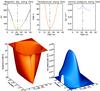 |
Fig. 7 Same as in Fig. 6 but for the Shallow_dip. |
| In the text | |
|
Fig. 8 Synthetic profiles produced by the Deep_dip. Lyman-α to Lyman-δ lines are plotted. For each line we plot synthetic profiles obtained at different positions along the x-axis with LOS oriented across the field lines (along the y-axis). Clearly reversed synthetic profiles are highlighted by red lines (only in the online version). |
| In the text | |
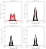 |
Fig. 9 Same as in Fig. 8 but for the Shallow_dip. |
| In the text | |
|
Fig. 10 Example of published observed Lyman line profiles obtained by SOHO/SUMER from May 25, 2005 prominence (left half), and Apr. 26, 2007 prominence (right half). Lyman-α to Lyman-δ line profiles are plotted for the first prominence, and Lyman-β to Lyman-δ line profiles are plotted for the second prominence. Each panel contains profiles from all pixels along the SUMER slit that belong to the observed prominence. |
| In the text | |
|
Fig. 11 Same as in Fig. 8 but for the Adapted_Model1. In addition, here we plot by black dashed lines, the temperature and gas pressure profiles of the KS-type Model1. |
| In the text | |
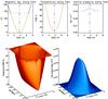 |
Fig. 12 Same as in Fig. 8 but for the Adapted_Model2. |
| In the text | |
Current usage metrics show cumulative count of Article Views (full-text article views including HTML views, PDF and ePub downloads, according to the available data) and Abstracts Views on Vision4Press platform.
Data correspond to usage on the plateform after 2015. The current usage metrics is available 48-96 hours after online publication and is updated daily on week days.
Initial download of the metrics may take a while.