| Issue |
A&A
Volume 546, October 2012
|
|
|---|---|---|
| Article Number | A9 | |
| Number of page(s) | 22 | |
| Section | Galactic structure, stellar clusters and populations | |
| DOI | https://doi.org/10.1051/0004-6361/201219853 | |
| Published online | 27 September 2012 | |
Spectral classification and HR diagram of pre-main sequence stars in NGC 6530⋆,⋆⋆,⋆⋆⋆
INAF – Osservatorio Astronomico di Palermo, Piazza del Parlamento, Italy 1, 90134 Palermo, Italy
e-mail: loredana@astropa.inaf.it
Received: 20 June 2012
Accepted: 3 August 2012
Context. Mechanisms involved in the star formation process and in particular the duration of the different phases of the cloud contraction are not yet fully understood. Photometric data alone suggest that objects coexist in the young cluster NGC 6530 with ages from ~1 Myr up to 10 Myr.
Aims. We want to derive accurate stellar parameters and, in particular, stellar ages to be able to constrain a possible age spread in the star-forming region NGC 6530.
Methods. We used low-resolution spectra taken with VLT/VIMOS and literature spectra of standard stars to derive spectral types of a subsample of 94 candidate members of this cluster.
Results. We assign spectral types to 86 of the 88 confirmed cluster members and derive individual reddenings. Our data are better fitted by the anomalous reddening law with RV = 5. We confirm the presence of strong differential reddening in this region. We derive fundamental stellar parameters, such as effective temperatures, photospheric colors, luminosities, masses, and ages for 78 members, while for the remaining 8 YSOs we cannot determine the interstellar absorption, since they are likely accretors, and their V − I colors are bluer than their intrinsic colors.
Conclusions. The cluster members studied in this work have masses between 0.4 and 4 M⊙ and ages between 1 − 2 Myr and 6 − 7 Myr. We find that the SE region is the most recent site of star formation, while the older YSOs are loosely clustered in the N and W regions. The presence of two distint generations of YSOs with different spatial distribution allows us to conclude that in this region there is an age spread of 6 − 7 Myr. This is consistent with the scenario of sequential star formation suggested in literature.
Key words: techniques: spectroscopic / open clusters and associations: individual: NGC 6530 / stars: formation / Hertzsprung-Russell and C-M diagrams / stars: pre-main sequence / stars: fundamental parameters
Based on observations collected at the European Southern Observatory, Paranal, under program ID 077.C-0073B.
Tables 1, 3, and 5 are available in electronic form at http://www.aanda.org
FITS files are only available at the CDS via anonymous ftp to cdsarc.u-strasbg.fr (130.79.128.5) or via http://cdsarc.u-strasbg.fr/viz-bin/qcat?J/A+A/546/A9
© ESO, 2012
1. Introduction
The study of very young open clusters is crucial to understanding the process of star formation within molecular clouds, since by measuring their age dispersion, it is possible to reconstruct the star formation history and test different star formation theories. A still controversial issue concerns the predictions of the duration of different phases of star formation. According to early models, clouds were considered in virial equilibrium, which makes them evolve on long time scales (≳108 years) (e.g. Solomon et al. 1979; Palla & Stahler 2000; Tan et al. 2006; Huff & Stahler 2007). In contrast, recent observations obtained with the Herschel observatory reveal very elongated, filamentary structures (e.g. Molinari et al. 2010), suggesting clouds affected by supersonic turbulence (Ballesteros-Paredes et al. 2007) that are expected to form stars on short time scales (~107 years) (e.g. Elmegreen 2000; Hartmann et al. 2001; Elmegreen 2007).
Reliable age determinations in star-forming regions are thus crucial to deriving the age spread and establish the duration of the star formation process. This allows us to constrain star formation theory and also to understand the evolution of the circumstellar material around young stellar objects (YSOs), which are strictly related to planet formation.
Stellar ages can be derived by different methods, as discussed in Soderblom (2010), but the physical complexity of YSOs and of their environment imply very large uncertainties on the stellar parameters from which ages are inferred (see Preibisch 2012, for a detailed review). The most widely used method of estimating the ages of young stars is to derive effective temperatures and luminosities from observational data and compare them in the Hertzsprung-Russell diagram (HRD) with those predicted by theoretical pre-main sequence (PMS) models. Uncertainties in the stellar parameters of SFRs, if not appropriately considered, can be underestimated leading to the interpretation of the observed scatter in the HRD as an intrinsic age spread rather than as un upper limit to the true age spread (Preibisch 2012).
One of the most important contributions on the stellar parameter uncertainties comes from the presence of different amount of interstellar and circumstellar extinction around YSOs. This yields highly unreliable derivations of effective temperature from photometric colors and therefore requires the acquisition of low-resolution spectra to derive spectral types to infer accurate effective temperatures. An appropriate reddening law to derive the absorption and therefore the luminosity, and a suitable treatment of other sources of uncertainties, such as excess emission in the blue and/or in the IR spectrum, binarity, and photometric variability are also crucial for deriving accurate stellar parameters, hence reliable stellar ages.
A good target for studying all these topics is the very young and rich open cluster NGC 6530 (associated with the giant molecular cloud M8 or Lagoon nebula), located about 1250 pc from the Sun. A peculiarity of this region is the presence of the Hourglass nebula, a compact H II region, produced by the extremely young O7.5 V star Herschel 36.
Several investigations have been devoted to this cluster since the work of Walker (1957). The main challenge when studying star-forming regions comes from most of the cluster stars still being in the PMS phase and, due to the age spread and/or observational uncertainties, are located in a broad region of the color-magnitude diagram (CMD). In the case of NGC 6530, only stars hotter than about A0 spectral types are located on the cluster main sequence, while most of the cluster members show a wide spread in the CMD. Sung et al. (2000) gives a list of 37 PMS candidates of NGC 6530, based on Hα and UBVRI photometry, down to V ~ 17. They also derived individual reddening values for 30 O and B type stars, finding evidence of differential reddening with E(B − V) in the range [0.25, 0.5] mag and a mean value of 0.35. More recently, a long list of candidate members (884 sources) has been obtained using a deep Chandra ACIS-I X-ray observation (Damiani et al. 2004). Optical and IR (2MASS) properties of these X-ray sources have been analyzed by us in Prisinzano et al. (2005) and in Damiani et al. (2006). Using BVI images taken with the WFI camera of the ESO 2.2 m telescope, we obtained a photometric catalog that reaches down to V ≃ 23, from which we derived a revised cluster distance of ≃ 1250 pc. This value has been confirmed by Arias et al. (2006) who derived the cluster distance using the spectral energy distribution, from optical and IR photometry, for a group of stars around Herschel 36. Adopting this distance value, the Sung et al. (2000) mean reddening and theoretical models, we estimated ages and masses from photometry and, within the large uncertanties derived by the assumption of a mean reddening, we found indications of a sequential star formation.
Few spectroscopic studies are available for the low-mass population of this cluster. In particular, 332 PMS candidates with V ≤ 18 mag, chosen based on their position in the color-magnitude diagrams, have been studied using high-resolution spectroscopic observations (R = 19 300) taken with GIRAFFE-FLAMES at the VLT, with the setup around the lithium line, and around the Hα line for a subsample of them (Prisinzano et al. 2007, hereafter PDM2007). Most of them (237) are confirmed cluster members based on their radial velocities and on the presence of a strong lithium line. However, most of the derived properties of the cluster (age spread, disk frequency, IMF, and history of star formation) are based on temperatures derived by the B − V and V − I colors, assuming a mean reddening, so they are affected by very large uncertainties.
Intermediate-resolution spectra in the range 3850–7000 Å of 39 YSOs in NGC 6530 with Hα emission and NIR excess were used by Arias et al. (2007) (hereafter ABM) to derive effective temperatures, luminosities, masses, and ages, by means of NIR photometry. Although the sample of studied members is relatively small, their results also suggest a sequential process in the star formation.
In this paper we present the spectral type classification of a selected sample of candidate members of NGC 6530 with a large number of relatively clean objects with X-ray emission but without evidence of NIR excesses and thus likely weak T Tauri stars (WTTS). In addition, we present results for YSOs with evidence of NIR excesses and for candidate YSOs selected from their position in the CMD. The aim of this work is to determine reliable and accurate effective temperatures and luminosities to be placed in the H-R diagram. In addition we want to investigate if a real age spread is present in this cluster and if the evidence of a sequential and triggered star formation from N to S, as found since the work of Lada et al. (1976), can be confirmed with our data.
2. Observations
2.1. Target selection
We observed a total of 94 spectroscopic targets, selected among candidate members with 12.5 < V < 19.0 in the PMS region of NGC 6530 by using the Prisinzano et al. (2005) optical catalog obtained from images taken with the WFI camera of the ESO 2.2 m telescope. Most of our targets (65) do not show strong IR excesses and were chosen for being likely clean YSOs not affected by severe veiling effects, for which the derived stellar parameters should be affected by relatively small uncertainties. In addition, we selected 24 candidate YSOs with evidence of NIR excesses in the JHK color − color diagram and five further targets selected because they fall in the PMS region of the V vs. V − I diagram.
Among our targets, 87 have an X-ray counterpart in Damiani et al. (2004), while 68 are in common with the sample of VLT/FLAMES spectra published in PDM2007.In Table 1 we list coordinates, literature identification number, and photometric data of our targets, and in Fig. 1 (top panel) we show the V vs. V − I diagram where candidates without and with NIR excesses and selected only photometrically are highlighted with different symbols.
2.2. Observations and data reduction
Spectroscopic observations of the NGC 6530 cluster were performed on May 25, 2006 and on June 17, 2006 within the ESO program 077.C-0073B, with the VIMOS instrument mounted at the Nasmyth focus B of the ESO-VLT UT3 telescope.
We used the multi-object spectroscopy (MOS) and high-resolution (HR) modes, with the Orange setup (spectral resolution R ~ 2150, with a slit width of 1 arcsec), covering a spectral range approximatevely between 5200 and 7600 Å. Slit definition and positioning were performed with the VIMOS Mask Preparation Software (VMMPS). Target positions were taken from the source list found in the VIMOS pre-imaging. Our targets were observed with three exposures of 2260 s. Further details are given on the log of observations given in Table 2.
Data were reduced with the VIMOS pipeline and the ESO Recipe Execution Tool (EsoRex). For the analysis of this work we considered the reduced spectra of detected objects. For the spectra obtained on May 29, calibration lamps were acquired after seven and ten hours from the first and second observations, respectively. As a consequence, the telescope rotator position was very different from the one at the time of the science spectra acquisition. Since the relative slit position with respect to the grism changes with the rotator position, these spectra are affected by a distortion that caused a variable shift along the dispersion direction up to 12 Å in the wavelength calibration. For this reason, our spectra were not summed to improve the S/N but were analyzed separately, and appropriate local wavelength corrections have been found, when required, for the analysis presented in this work.
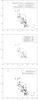 |
Fig. 1 V vs. V − I diagram of our targets. Top panel shows the 65 targets classified as candidate weak T Tauri stars, since they were detected in the X-rays, the 21 targets with IR excesses and the five photometric candidates, selected for the VIMOS observations. Middle panel shows the CMD for the 68 targets, also observed with FLAMES were “M” indicates the 63 confirmed cluster members, “NM” indicates the three nonmembers and “M?” indicates the two uncertain members. Bottom panel shows the CMD for the 88 targets classified here as cluster members and the six classified as nonmembers. |
Log of the VIMOS observations.
3. Results
3.1. Identification of cluster members
For the 68 objects observed with both instruments (VIMOS, this work and FLAMES, Prisinzano et al. 2007), the cluster membership has been established by using the results from the FLAMES high-resolution spectra obtained by Prisinzano et al. (2007), based on radial velocities and on the equivalent width of the Li I absorption line at 6707.8 Å. Figure 1 (middle panel) shows the V vs. V − I diagram of the VIMOS targets with a counterpart in Prisinzano et al. (2007), where 63 of them were classified as confirmed cluster members (“M”), three as cluster nonmembers (“NM”) and two with uncertain membership (“M?”).
In this work, we consider confirmed cluster members the 63 objects labeled in PDM2007 with “M” and the star ID = 24 labeled with “M?” for its discrepant radial velocity. Among the confirmed members we include the star with ID = 19 that was classified in PDM2007 as a nonmember since this star does not show any X-ray detection, Li line, or Hα broadening in the FLAMES spectrum; neverthless, the VIMOS spectrum shows an evident Li absorption and a broad Hα in emission with FWZI ~ 17 Å. After careful analysis of the FLAMES spectrum we noted that the whole spectrum shows very few lines, and we suspect there is a problem in the fiber assignment for this star. Thus we classify the star with ID = 19 here as a confirmed cluster member.
For those spectra that we only observed spectroscopically with VIMOS, we established the membership status by considering the presence of the X-ray detection and by inspecting the presence of the Li I absorption line at 6707.8 Å and the shape of the Hα line. Unfortunately, we cannot measure the equivalent width of the Li I, since the spectral resolution of our spectra is too low to resolve this line, which is blended with the nearby iron lines (Fe I 6705, 6710 Å, Covino et al. 1997). However, since the Li I line is expected to be very strong for late type YSOs, as are many of our targets, we used this line to assert the membership for the 26 objects for which we do not have high-resolution spectra.
For YSOs, emission lines and, in particular, the Hα line, are good indicators of youth, but in the case of NGC 6530, emission lines cannot be used as membership indicators, since the spectra may suffer from Hα line contamination from the surrounding Lagoon nebula. Owing to its strong spatial variability, the subtraction of the nebula contribution is not reliable, and thus we did not attempt to improve the sky subtraction obtained with the recipes of the VIMOS pipeline. Neverthless, the Hα line from the nebula is expected to be narrow, while that from YSOs with accretion is expected to be widened at the continuum level thanks to the gas motion in the circumstellar regions. Even if it is very hard to accurately measure the full width at zero intensity (FWZI) in low-resolution spectra, we inspected the base of the Hα line, so we considered cluster members those with a broad line, i.e., those with FWZI ≥ 10 Å.
In conclusion, we consider nonmembers to be the following objects: stars ID = 15 and 70, already classified as “NM” in PDM2007 for the absence of the Li line, the lack of X-ray detection, and the Hα in absorption; stars ID = 8, 23, 51, and 92 for the absence of the Li line in the VIMOS spectrum and the narrow FWZI of the Hα line.
The V vs. V − I diagram of the 88 confirmed cluster members and of the six nonmembers is shown in Fig. 1 (bottom panel).In Table 3 we list members and nonmembers selected in PDM2007 and those identified in this work.
3.2. Spectral classification
Spectral types of the observed objects were determined by using the MILES stellar library (Sánchez-Blázquez et al. 2006) whose spectra cover the range [3525 − 7500] Å at 2.50 Å (FWHM) spectral resolution, which is similar to that of our spectra. The library includes 985 spectra of dwarfs, giants, and subgiants spanning a wide range in atmospheric parameters. For the present analysis we selected only spectra of nonvariable stars with −0.3 < [Fe/H] < 0.3, i.e. with solar-like metallicity and MK spectral types from B1 to M61.
The properties of lines in stellar spectra are very sensitive to the luminosity class, and thus the spectral classification, especially for contracting YSOs with expected low gravity, can be reliable only if we compare spectra with the same luminosity class. To this aim we used the Ca I triplet lines (6102, 6122, 6162 Å) since these lines are very strong in giants, and the wing profile is sensitive to the surface gravity (Edvardsson 1988). In particular, we computed the ratios of the intensity of the three Ca I lines over the intensity of the nearby Fe I line at 6137 Å by using spectra normalized to the continuum in a region of 40 Å around each line. Figure 2 shows these ratios for the standards as a function of spectral type for the giants and main sequence stars. The plots show that these ratios can be used as diagnostics of luminosity class as for objects later than G7.
We computed the same ratios for the spectra of our targets and found that only the stars with ID = 74, 82, and 89 are compatible with the trend of giants, while all the other objects can be classified as main sequence stars.
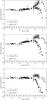 |
Fig. 2 Ratios of the three Ca I line intensities at 6102.7 (top panel), 6122.0 (middle panel), and 6162.0 Å (bottom panel), respectively, with respect to the Fe I line at 6137 Å, used to determine the luminosity class of our targets. |
Spectral classification is usually based on the comparison of lines forming in the stellar atmosphere, but in PMS stars the presence of additional lines originating in the circumstellar or interstellar material implies one difficulty in determining spectral types. Thus the comparison of our spectra with the standard ones has been made by excluding the following regions (which include also several telluric lines): (a) 6270–6300 Å, around the O2 telluric line at 6277 Å (Conti et al. 1995); (b) 6850–6930 Å, and 7570–7700 Å, including the O2 B and A bands (Jao et al. 2008); (c) 7150–7220 Å, including the H2O absorption (Sánchez-Blázquez et al. 2006); (d) 5773–5800 Å, including the diffuse interstellar features at 5780 and 5797 Å (Wallerstein & Cardelli 1987); (e) 5875–5905 Å around the Na I D1 D2 lines at 5890, 5896 Å, which may be produced also in the circumstellar environment. Finally we also excluded the Hα line and the region 6702–6712 Å around the Li I, which is very strong only in YSOs, while it is not present in the standard spectra. We did not consider those emission lines typical of YSOs (see Col. 3 in Table 4), since not all spectra show them, and they can originate from the hot circumstellar material and/or from the surrounding nebula.
Spectral comparison has been made by splitting each spectrum in the spectral regions 5020–5500, 5500–6000, 6000–6500, 6600–6850, 6930–7550, and 7750–8100 Å2, which were normalized to the continuum with IDL by using the same parameters (an order 3 polynomial function) for both the standards and our targets. For each target and for each spectral range, we computed the difference between the target spectrum and the standard ones to compute the residuals. Classification has been established by considering the spectral type of the standard giving the minimum rms of the residuals. Results have been checked by a visual inspection of the residuals.
The normalization can be problematic for stars later than K7 V, where the TiO and VO molecular bands appear to be deeper towards later spectral types. However, since we used the same parameters and the same spectral ranges, the resulting continuum normalization of target and standard spectra can be used in order to estimate the difference among the spectra. Uncertainties were assigned on the basis of the goodness of the comparison with the standard spectra.
This method is efficient to classify K and M stars whose spectra show several lines but give very large uncertainties for earlier type stars. Thus, for the few objects (10) with spectral type earlier than K, we used a second method based on the intensities of the lines given in Table 4 as a function of the spectral types of the standar stars. We measured the intensity of these lines on the spectra normalized to the continuum by using 20 spectral ranges of width from 30 to 50 Å around the adopted lines. For each line and for each target a spectral type has been estimated by comparison with the trend of the intensity obtained for the standards. The final spectral type of each target has been established as the most recurrent value by considering all the adopted lines.
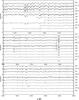 |
Fig. 3 Spectra of cluster members with spectral type between F0 and K2, in the region 5020 − 6500 Å, normalized to the continuum and arbitrally shifted for clarity. |
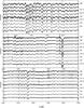 |
Fig. 4 Spectra of cluster members with spectral type between K2.5 and M0, in the region 5020 − 6500 Å, normalized to the continuum and arbitrally shifted for clarity. |
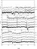 |
Fig. 5 Spectra of cluster members with spectral type between M0.5 and M4, in the region 5020 − 6500 Å, normalized to the continuum and arbitrally shifted for clarity. |
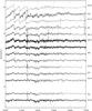 |
Fig. 6 Spectra of cluster members with spectral type between K2.5 and M4, in the region 7000 − 7500 Å, normalized to the continuum and arbitrally shifted for clarity. |
Typical lines found in our target spectra.
The results of our spectral classification are given in Table 3. Figures 3–6 show the spectra of cluster members normalized to the continuum in the spectral regions mainly used for the spectral classification. For each spectral type, spectra have been arbitrally shifted for clarity. Objects of the same spectral type are shifted by the same amount. In some cases, emission lines originating in the nebula and/or the circumstellar disk can be found in absorption. This is likely due to an overestimate of the sky subtraction for these objects.
Figure 7 shows the histogram of the spectral types derived in this work. The sample is dominated by K and M stars, which total 42 and 32, respectively. Among the cluster members, we were not able to classify the Class 0/I star with ID = 31, since the spectrum show only emission lines and star with ID = 46, which it is likely a high rotator, so it shows very few lines.
3.3. Veiling
Spectra of YSOs can be affected by veiling, i.e. a contribution to the continuum, likely from the material falling towards the inner star along columns beamed by the magnetic field. The total accretion column emission can be described by an optically thick emission originating in the heated photosphere and by an optically thin emission due to the infalling material (Calvet & Gullbring 1998). For the aim of our work, in case of veiling we can have two effects: first, a change in the photospheric optical magnitudes owing to an excess in the blue part of the spectrum; and second, a wrong spectral type determination since in the case of veiling, lines can appear weaker. This can lead to attributing an earlier spectral type than the true one.
A detailed analysis of the possible role of the accretion in the BVI bands was conducted by Da Rio et al. (2010), who simulated a typical accretion spectrum and added it to a reference model for the photospheric colors of YSOs in the Orion nebula cluster. They calculated the displacement in the V − I vs. B − V diagram caused by the presence of ongoing accretion assuming different ratios of the accretion luminosity with respect to the total luminosity. Their results show that the effect is greater on the B − V than on the V − I and that even an accretion luminosity lower than 10% of the total luminosity of the star has a strong effect on the colors of low-temperature stars.
To highlight the presence of possible objects with large veiling in our sample, we compared the V − I and B − V colors of our targets with the locus of photospheric colors from Kenyon & Hartmann (1995) of main sequence stars reddened by using the mean cluster reddening E(B − V) = 0.35 (Sung et al. 2000), as shown in Fig. 8, and the Munari & Carraro (1996) reddening law for RV = 5.0 (see Sect. 3.5), since this is the one that follows the bulk of our data better.
From this plot we find that six objects show an evident excess in the optical colors, as indicated in Table 3. Three of them (ID = 4, 74, 93) also show a broad Hα line while 4 were classified by us as class II YSOs for their NIR excesses. For these objects we have strong indicators of membership with evidence of accretion, but we cannot estimate reliable photospheric parameters, so they will be considered with caution in the following analysis.
Figure 8 also shows that the bulk of our data follows the reddening direction and, within the possible spread due to the uncorrect reddening, they do not show any strong excesses with respect to the expected photospheric colors. Thus we can consider the magnitudes of these objects representative of their photosphere and can be used to derive reliable stellar parameters (see Sect. 3.5 for a detailed discussion).
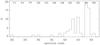 |
Fig. 7 Histogram of the spectral types found by using the VIMOS spectra. |
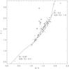 |
Fig. 8 V − I and B − V diagram of NGC 6530 members presented in this work. Solid line is the locus of photospheric colors from Kenyon & Hartmann (1995) reddened by using the mean cluster reddening E(B − V) = 0.35 (Sung et al. 2000) and the Munari & Carraro (1996) reddening law for R = 5.0 (see Sect. 3.5). The reddening vector assuming E(B − V) = 1 is also drawn. Empty circles indicate objects with evident excess in the optical colors. |
As already mentioned, a further effect of a possible veiling is an unrealistic spectral type classification. Nevertheless, as described in Sect. 3.2 for each objects, we split the whole spectrum into more regions and verified that the adopted final spectral type is consistent in every subspectrum, by considering that some spectral regions are more sensitive to veiling than others, depending on the spectral type. In particular, since most of our targets are late K and M stars, we mainly used the reddest part of the spectrum – more sensitive for these spectral types–, which is expected to be less affected by veiling (Gullbring et al. 2000). In addition, since most of our targets are candidate class III YSOs, with no strong evidence of a circumstellar disk, we can conclude that our spectral classification should not be influenced by the veiling, with the exception of the star with ID = 31, which we were not able to classify since its spectrum shows only emission lines. This object was classified as class 0 by Kumar & Anandarao (2010) by using IRAC-Spitzer photometry.
In addition we find that star ID = 86 shows a very peculiar spectrum with the reddest region (6900 − 7400 Å) similar to that of K7-M0.5 V star, the region 6000–6500 Å similar to a K3-K4 V star, while the region 5000–5500 Å similar to a G8 V star. Since the FWZI is quite high (19 Å), we guess that this object is affect by veiling and/or variability. Given its previous spectral classification (B8.5 V from SIMBAD database) and its bright magnitude, we do not exclude this object being a candidate FU-Ori object or a binary where we can see the low-mass companion spectrum. Based on inconsistent features in their spectra, we also suspect a possible effect of veiling for the stars ID = 12 and 36. Even in this case, we consider these objects with caution for the following analysis.
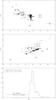 |
Fig. 9 E(V − I) vs. intrinsic (V − I)0 (top panel) and vs. observed (V − I) (middle panel). Objects indicated by empty diamonds are M0 or later stars. The reddening vector corresponding to E(V − I) = 1 is also plotted. E(V − I) distribution (bottom panel) obtained by considering all targets (dotted line) and the selected sample including the 70 cluster members with E(V − I) > 0 and without special photometric or spectroscopic features indicated in Table 3. |
3.4. Intrinsic colors and reddening
To convert spectral types into intrinsic colors, we used the Kenyon & Hartmann (1995) transformations. We verified that for the colors of our targets, the Kenyon & Hartmann (1995) relation is very similar to that suggested in Luhman (1999), which considers the Kenyon & Hartmann (1995) colors for types earlier than M0 and the colors from Leggett (1992) for M0 and later types. Figure 9 shows individual reddenings E(V − I), derived from the difference between the observed and the intrinsic colors, as a function of the intrinsic (V − I)0 (top panel) and of the observed (V − I) (middle panel).
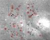 |
Fig. 10 Spatial distribution of all the objects studied in this work overplotted on the combination of the two deep-dithered I band WFI images (Prisinzano et al. 2005). X symbols indicate WTTS, circles indicate CTTS, plus indicate nonmembers, and diamonds indicate M0 or later stars. O stars falling in the field of view (FOV) investigated in this work are also indicated. Coordinates RA(J2000) and Dec(J2000) are given in hours and degrees, respectively. |
In Fig. 9 we also have unphysical negative reddening values for a few members. We find that the seven YSOs with E(V − I) < 0 are all YSOs of spectral type equal or later than M0, and two of them show a quite high FWZI of Hα (>15 Å). We guess that these negative values are due to observed colors that are bluer than the pure photospheric ones for a possible excess in the V band owing to accretion processes. This is expected for late type stars, since, as shown in Da Rio et al. (2010), low fractions of accretion luminosity have a strong effect on the colors of low-temperature stars.
In Fig. 9 (middle panel), all objects follow the reddening vector, but the mean reddening of M stars is lower than the one of earlier type stars, and the two populations are quite distinct. This is a selection effect, since M stars more reddened than the observed ones would be fainter than our observational limit. This is consistent with the spatial distribution of the objects studied in this work, shown in Fig. 10, where M type stars are homogeneously distributed in the N and E regions but are almost completely absent in the SW region, where the mean reddening is higher and/or the sensitivity is lower for the strong nebular Hα emission.
Finally, Fig. 9 (bottom panel) shows the reddening distribution by considering the whole sample and the subsample of 78 cluster members with E(V − I) > 0, which we will indicate hereafter as the selected sample. If we consider this subsample, we find a mean value of E(V − I) = 0.7 with an rms equal to 0.5. By using the adopted reddening laws, the mean value corresponds to E(B − V) = 0.42, which, within the errors, is consistent with the value ⟨ E(B − V) ⟩ = 0.35 found by Sung et al. (2000).
3.5. Reddening law
To derive stellar luminosities, we also need to know the interstellar absorption, which can be derived from the reddening values. This step requires assuming a suitable reddening law (RV), which, in many star-forming clouds, has been proved to be different from the standard interstellar extinction law (Povich et al. 2011). In addition, very recently, Fernandes et al. (2012) has suggested for NGC 6530 an anomalous extinction law (RV = 4.5) by using the distribution of known E(V − K) vs. E(B − V) values. Their sample is, however, limited to objects with E(B − V) ≲ 0.4.
To constrain the reddening law adequate for this cluster, we used the ratios E(V − I)/E(B − V) and E(V − K)/E(B − V). In fact, for weak T-Tauri stars, the observed colors should only be affected by interstellar absorption and the reddening ratios derived by using different colors should be sensitive to the total-to-selective extinction RV, which depends on composition and size of the grain in the interstellar medium. For example, Fitzpatrick & Massa (2009) suggest to use the relation 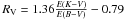 to derive the reddening law.
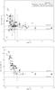 |
Fig. 11 Color excess ratios as a function of E(B − V) computed for our targets. Horizontal solid lines indicate the color excess ratios predicted by the Munari & Carraro (1996) (top panel) and Fiorucci & Munari (2003) (bottom panel) reddening laws for RV = [3.1,5.0] . |
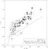 |
Fig. 12 J − H vs. H − K diagram of our targets. The solid curve is the Kenyon & Hartmann (1995) locus for the colors of main sequence stars, the two arrows indicate the reddening vectors corresponding to AV = 3 starting from colors of M0 and M2 dwarfs, and the solid line is the CTTS locus by Meyer et al. (1997). |
To this aim, we selected cluster members with E(B − V) > 0. In addition, we discarded peculiar objects with features reported in the notes of Table 3. Figure 11 shows E(V − I)/E(B − V) (top panel) and E(K − V)/E(B − V) (bottom panel) as a function of E(B − V). Candidate accretors, defined as objects with an FWZI in the the Hα line higher than 10 Å, and objects with IR excesses are indicated by different symbols. The ratios E(V − I)/E(B − V) = [1.25,1.66] and E(V − K)/E(B − V) = [2.73,4.45] for RV = [3.1,5.0] , by using the Munari & Carraro (1996) reddening law for the optical bands and the Fiorucci & Munari (2003) for the 2MASS bands are also indicated in the figure. The extinction coefficients by Munari & Carraro (1996) and Fiorucci & Munari (2003) were derived by using the Mathis (1990) and Fitzpatrick (1999) reddening laws, respectively, weighted over the V RC IC and J H KS band profiles of the Bessell (1976) and 2MASS photometric systems, respectively.
We find that only a fraction of our targets show color-excess ratios consistent with uniform RV, as expected for normal reddened stars, while for many objects the color excess ratios show a wide spread that it is likely due to excesses in the blue B and/or in the red K bands. In fact, most of the accretors have high E(V − I)/E(B − V), while almost all the objects with IR excesses have high E(V − K)/E(B − V).
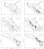 |
Fig. 13 V vs. V − I diagram obtained by using observed (top panels) and dereddened (middle panels) magnitudes and colors for the CTT and WTT cluster members with E(V − I) > 0. Solid and dotted lines are the Siess et al. (2000) isochrones and track, respectively, assuming the cluster distance of 1250 pc (Prisinzano et al. 2005). In the top panel, the isochrones are reddened by assuming the literature mean reddening E(B − V) = 0.35 (Sung et al. 2000) and the Munari & Carraro (1996) reddening laws for RV = 5.0. In the middle panel, isochrones are only scaled for the cluster distance. The arrow indicates the reddening vector corresponding to E(B − V) = 0.35 for RV = 5.0. The HR diagrams of the two samples are shown in the bottom panels. |
Objects with evident NIR excesses can also be seen in Fig. 12 where we show the J − H vs. H − K diagram. Most of our targets show colors that are more reddened than those expected for dereddened main sequence stars. Nevertheless, since our targets are YSOs of earlier spectral type than M2, the observed colors cannot be explained by interstellar reddening alone, as can be seen by the comparison with the reddening vectors. Instead, for many of our targets, the observed colors are consistent with the Meyer et al. (1997) locus of CTTS stars. Therefore, the observed colors result from a combination of interstellar reddening and NIR excesses from dust of the circumstellar disk.
However, if we consider the objects with constant color excess ratios we find that the values E(V − I)/E(B − V) are consistent with the ratio given by Munari & Carraro (1996) for RV = 5.0, while if we consider the objects with E(K − V)/E(B − V) < 4, we find RV in the range 4.0–4.5 by using the Fitzpatrick & Massa (2009) equation. Since our sample is dominated by YSOs with circumstellar disk with or without excesses, we cannot constrain the RV value with high precision. Nevertheless, by considering the consistency of the results obtained both from optical and IR magnitudes, we can conclude that NGC 6530 cluster members show an anomalous extinction with RV ≲ 5.0. Thus for the following analysis, we use the reddening ratios given by Munari & Carraro (1996) for RV = 5.0.
4. Discussion
4.1. H-R diagram, ages, and age spread
Figure 13 shows the observed (top panels) and dereddened (middle panels) color − magnitude diagrams for the 21 CTTS (left panels) and the 57 WTTS (right panels) members with E(V − I) > 0. The sample of CTTS includes an object classified as Class 0/I based on the IRAC-Spitzer photometry (Kumar & Anandarao 2010). The HR diagrams of the two samples are shown in the bottom panels. Effective temperatures and bolometric corrections were derived by using the Kenyon & Hartmann (1995) transformations. Bolometric luminosities were determined from the V magnitudes, by considering individual absorption corrections derived by the intrinsic colors and the adopted reddening law. Masses and ages were derived by interpolating the theoretical tracks and isochrones by Siess et al. (2000) to the position of the stars in the V0 vs. (V − I)0 diagram. Uncertainties on the stellar parameters were derived by propagating individual uncertainties on the spectral types. The values of individual extinctions, effective temperatures, bolometric luminosities, ages and masses, and the relative uncertainty ranges are given inTable 5.
The comparison between the two CMDs (observed and dereddened) drawn in Fig. 13 shows that the actual dynamic range of the intrinsic magnitudes (V0 = 10. − 18.1) is greater than that of the observed magnitudes (V = 14.5 − 19.0). In addition, we note that the individual correction for interstellar reddening allows us to reduce the apparent age spread, since we find that most of those YSOs that in the V vs. V − I diagram have an apparent age in the range 0.1–1 Myr are actually very reddened stars with age ≳ 1 Myr. Finally, we see that the mass distributions in the observed and dereddened diagrams are very different.
Figure 14 shows the (cumulative) age distributions for the WTTS and CTTS and for the joint sample (WTTS plus CTTS). The ages of WTTS are not significantly different from the CTTS ones, with a marginal indication that CTTS are younger than WTTS. As a result, we decided to consider the WTTS-plus-CTTS joint sample and found that around 60% of cluster members have ages in the range ~1–2 Myr, but there is an older population with ages in the range 3–7 Myr. Even if a small part of this spread (~1.5 Myr) could be attributed to binaries, we exclude the younger population actually being a population of binaries, since in this case the two populations should have the same spatial distribution.
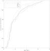 |
Fig. 14 Cumulative age distribution of WTTS, CTTS and all cluster members. |
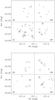 |
Fig. 15 Spatial distribution of the populations youngest (top panel) and oldest (bottom panel) than 2.0 Myr (empty circles). Different circle sizes correspond to objects with E(V − I) < 0.5 (smallest circles), 0.5 ≤ E(V − I) < 1.0 (medium circles) and E(V − I) ≥ 1 (largest circles). X symbols indicate objects with mass larger than 2.5 M⊙. The four regions corresponding to the four VIMOS CCD quadrants are also indicated. |
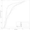 |
Fig. 16 Cumulative age distribution of all objects in the four spatial regions shown in Fig. 15. The cumulative age distributions of all the objects located in the SE and in the other regions and of the combined SW-NW-NE sample are also shown. |
This is not the case, as shown in Fig. 15 where we plot the spatial distributions of the YSOs with ages younger and older than 2 Myr falling in the N, S, W, and E regions corresponding to the four VIMOS CCD quadrants. Different symbol sizes correspond to YSOs with E(V − I) in the ranges indicated in the caption. We find that, while the oldest objects are quite homogeneously located in the observed region, about 50% of the youngest objects (ages < 2 Myr) are located in the SE region. To see whether the spatial distribution of the youngest population is significantly different from the oldest one, we derived the cumulative age distribution in the four regions shown in Fig. 16. Since the number of objects in the N and SW region is very small, we also consider the sample including all the objects in these three regions with the aim to have more robust statistical results. From these distributions, it is clear that in the SE region around 80% of the objects are younger than 2 Myr, while this percentage is much lower (~40–50%) in the other regions. Using the two sample Kolmogorov-Smirnov tests, we find that the population of objects in the SE is different from the one in the SW-NE-NW regions at a significance level of 99%. Figure 15 also shows that there is no correlation between the spatial distribution of the individual reddenings and the one of the derived ages, so we can discard the observed “age spread” as due to an artifact from the treatment of the extinction.
Our results support the scenario of sequential star formation since we find a first generation of stars in the N regions and in the SW region and a second generation of stars that is quite concentrated in the SE region. Since our observations do not cover the central region, we cannot say anything about this interesting region.
Since the E(V − I) median value ± 1σ is equal to 0.52 , corresponding to
  , our observational limit implies a mass limit equal to 0.6
 M⊙ at 4 Myr, not including outliers that can have very different values of E(V − I) and mass limit. For these reasons, we are not able to discuss the sequential process as a function of stellar masses, even if we find that almost all seven observed YSOs with masses higher than 2.5 M⊙ are located in the SE region.
Our finding allows us to suppose that (within the FOV studied in this work) the SE region is the most recent site of star formation of low and intermediate mass stars where the population has not yet undergone (or just started) mass segregation. In contrast, the oldest population is more loosely clustered in the surrounding N and SE regions.
5. Summary and conclusions
We used the VLT/VIMOS spectra of 94 candidate cluster members of the young open cluster NGC6530 with the aim to obtain the spectral classification, crucial for deriving accurate stellar parameters. First of all, we considered available membership indicators (X-ray detection, radial velocities, lithium line, and Hα shape) both from literature data and/or from our new spectra to find members. Our spectral resolution does not allow us to measure the equivalent width of the lithium line, but since this line is expected to be very prominent in YSOs, we were able to use it effectively to distinguish cluster members.
Owing to the strong and spatially variable Hα emission from the surrounding nebula, we cannot quantify the Hα emission of the YSOs that are undergoing accretion, so we were not able to estimate the mass accretion rates. Nevertheless, we can distinguish strong accretors by estimating the FWZI of the Hα line that for these objects is larger than Hα emission coming from the nebula. Based on the available membership indicators, we find that 88 of our targets are confirmed cluster members, and the remaining six are nonmembers.
Based on the comparison with standard spectra in the literature, we classified our targets and found that the cluster member sample (88 YSOs) is dominated by late type stars with 42 K type and 32 M type stars, while for two of them we were not able to assign a spectral type.
By considering the Kenyon & Hartmann (1995) transformations, we derived intrinsic colors (V − I)0, hence the interstellar reddening E(V − I). We used the V − I colors, since they should be less affected by blue excesses due to accretion phenomena and by IR excesses from circumstellar disk dust. Even if our sample is dominated by WTTS, we find that some objects show evident blue excesses with respect to the locus of (V − I) vs. (B − V) colors, while eight YSOs have observed colors bluer than the intrinsic ones that would imply an unphysical negative reddening. This means that these objects are likely accretors in which the V − I colors include a contribution originating in the accretion hot spot. For these objects we did not attempt to derive stellar parameters since we cannot estimate the true interstellar absorption and get a reliable bolometric luminosity.
By considering only the 78 YSOs with E(V − I) > 0, we find a mean cluster reddening E(V − I) = 0.7 ± 0.5. In addition, by comparing the ratios E(V − I)/E(B − V) and E(V − K)/E(B − V), we conclude that the NGC 6530 members show an anomalous extinction with  . Therefore, for our analysis we used the reddening law given by Munari & Carraro (1996) for RV = 5.0. The mean cluster reddening corresponds to E(B − V) = 0.42, which is consistent with the value ⟨ E(B − V) ⟩ = 0.35 found by Sung et al. (2000). For this sample we derived fundamental stellar parameters, i.e. effective temperatures, interstellar absorption, luminosities, ages, and masses. The HR diagram shows that our targets have ages between about 1 and 6 − 7 Myr. There is not a significant difference of ages between WTTS and CTTS, but if we distinguish the populations younger and older than 2 Myr, we find that the youngest population is mainly concentrated in the SE region, while the oldest population is loosely clustered in the N and SW regions. Since the ages of two populations are significantly different, we can conclude that there are two generations of stars in this region, formed during different events. The SE region is therefore the most recent site of star formation in the FOV studied in this work. Our results confirm the scenario of sequential star formation already suggested in previous works.
Online material
List of stars observed with VIMOS.
Results on membership, spectral types, and Hα properties.
Acknowledgments
Part of this work was financially supported by the ASI contract I/044/10/0. We wish to thank C. Argiroffi for her help in some steps of the spectral classification.
References
- Arias, J. I., Barbá, R. H., Maíz Apellániz, J., Morrell, N. I., & Rubio, M. 2006, MNRAS, 366, 739 [NASA ADS] [CrossRef] [Google Scholar]
- Arias, J. I., Barbá, R. H., & Morrell, N. I. 2007, MNRAS, 374, 1253 [NASA ADS] [CrossRef] [Google Scholar]
- Ballesteros-Paredes, J., Klessen, R. S., Mac Low, M.-M., & Vazquez-Semadeni, E. 2007, Protostars and Planets V, 63 [Google Scholar]
- Bessell, M. S. 1976, PASP, 88, 557 [NASA ADS] [CrossRef] [Google Scholar]
- Calvet, N., & Gullbring, E. 1998, ApJ, 509, 802 [NASA ADS] [CrossRef] [Google Scholar]
- Conti, P. S., Hanson, M. M., Morris, P. W., Willis, A. J., & Fossey, S. J. 1995, ApJ, 445, L35 [NASA ADS] [CrossRef] [Google Scholar]
- Covino, E., Alcala, J. M., Allain, S., et al. 1997, A&A, 328, 187 [NASA ADS] [Google Scholar]
- Da Rio, N., Robberto, M., Soderblom, D. R., et al. 2010, ApJ, 722, 1092 [NASA ADS] [CrossRef] [Google Scholar]
- Damiani, F., Flaccomio, E., Micela, G., et al. 2004, ApJ, 608, 781 [NASA ADS] [CrossRef] [Google Scholar]
- Damiani, F., Prisinzano, L., Micela, G., & Sciortino, S. 2006, A&A, 459, 477 [NASA ADS] [CrossRef] [EDP Sciences] [Google Scholar]
- Edvardsson, B. 1988, A&A, 190, 148 [NASA ADS] [Google Scholar]
- Elmegreen, B. G. 2000, ApJ, 530, 277 [NASA ADS] [CrossRef] [Google Scholar]
- Elmegreen, B. G. 2007, ApJ, 668, 1064 [NASA ADS] [CrossRef] [Google Scholar]
- Fernandes, B., Gregorio-Hetem, J., & Hetem, Jr, A. 2012, A&A, 541, A95 [NASA ADS] [CrossRef] [EDP Sciences] [Google Scholar]
- Fiorucci, M., & Munari, U. 2003, A&A, 401, 781 [NASA ADS] [CrossRef] [EDP Sciences] [Google Scholar]
- Fitzpatrick, E. L. 1999, PASP, 111, 63 [NASA ADS] [CrossRef] [Google Scholar]
- Fitzpatrick, E. L., & Massa, D. 2009, ApJ, 699, 1209 [NASA ADS] [CrossRef] [Google Scholar]
- Gullbring, E., Calvet, N., Muzerolle, J., & Hartmann, L. 2000, ApJ, 544, 927 [NASA ADS] [CrossRef] [Google Scholar]
- Hartmann, L., Ballesteros-Paredes, J., & Bergin, E. A. 2001, ApJ, 562, 852 [NASA ADS] [CrossRef] [Google Scholar]
- Huff, E. M., & Stahler, S. W. 2007, ApJ, 666, 281 [NASA ADS] [CrossRef] [Google Scholar]
- Jao, W.-C., Henry, T. J., Beaulieu, T. D., & Subasavage, J. P. 2008, AJ, 136, 840 [NASA ADS] [CrossRef] [Google Scholar]
- Kenyon, S. J., & Hartmann, L. 1995, ApJS, 101, 117 [NASA ADS] [CrossRef] [Google Scholar]
- Kumar, D. L., & Anandarao, B. G. 2010, MNRAS, 407, 1170 [NASA ADS] [CrossRef] [Google Scholar]
- Lada, C. J., Gottlieb, C. A., Gottlieb, E. W., & Gull, T. R. 1976, ApJ, 203, 159 [NASA ADS] [CrossRef] [Google Scholar]
- Leggett, S. K. 1992, ApJS, 82, 351 [NASA ADS] [CrossRef] [Google Scholar]
- Luhman, K. L. 1999, ApJ, 525, 466 [NASA ADS] [CrossRef] [Google Scholar]
- Mathis, J. S. 1990, ARA&A, 28, 37 [NASA ADS] [CrossRef] [Google Scholar]
- Meyer, M. R., Calvet, N., & Hillenbrand, L. A. 1997, AJ, 114, 288 [NASA ADS] [CrossRef] [Google Scholar]
- Molinari, S., Swinyard, B., Bally, J., et al. 2010, A&A, 518, L100 [NASA ADS] [CrossRef] [EDP Sciences] [Google Scholar]
- Munari, U., & Carraro, G. 1996, A&A, 314, 108 [NASA ADS] [Google Scholar]
- Palla, F., & Stahler, S. W. 2000, ApJ, 540, 255 [NASA ADS] [CrossRef] [Google Scholar]
- Povich, M. S., Townsley, L. K., Broos, P. S., et al. 2011, ApJS, 194, 6 [NASA ADS] [CrossRef] [Google Scholar]
- Preibisch, T. 2012, Res. Astron. Astrophys., 12, 1 [NASA ADS] [CrossRef] [Google Scholar]
- Prisinzano, L., Damiani, F., Micela, G., & Sciortino, S. 2005, A&A, 430, 941 [NASA ADS] [CrossRef] [EDP Sciences] [Google Scholar]
- Prisinzano, L., Damiani, F., Micela, G., & Pillitteri, I. 2007, A&A, 462, 123 [NASA ADS] [CrossRef] [EDP Sciences] [Google Scholar]
- Sánchez-Blázquez, P., Peletier, R. F., Jiménez-Vicente, J., et al. 2006, MNRAS, 371, 703 [NASA ADS] [CrossRef] [Google Scholar]
- Siess, L., Dufour, E., & Forestini, M. 2000, A&A, 358, 593 [NASA ADS] [Google Scholar]
- Soderblom, D. R. 2010, ARA&A, 48, 581 [NASA ADS] [CrossRef] [Google Scholar]
- Solomon, P. M., Sanders, D. B., & Scoville, N. Z. 1979, in The Large-Scale Characteristics of the Galaxy, ed. W. B. Burton, IAU Symp., 84, 35 [NASA ADS] [Google Scholar]
- Sung, H., Chun, M.-Y., & Bessell, M. S. 2000, AJ, 120, 333 [NASA ADS] [CrossRef] [Google Scholar]
- Tan, J. C., Krumholz, M. R., & McKee, C. F. 2006, ApJ, 641, L121 [NASA ADS] [CrossRef] [Google Scholar]
- Wallerstein, G., & Cardelli, J. A. 1987, AJ, 93, 1522 [NASA ADS] [CrossRef] [Google Scholar]
All Tables
All Figures
|
Fig. 1 V vs. V − I diagram of our targets. Top panel shows the 65 targets classified as candidate weak T Tauri stars, since they were detected in the X-rays, the 21 targets with IR excesses and the five photometric candidates, selected for the VIMOS observations. Middle panel shows the CMD for the 68 targets, also observed with FLAMES were “M” indicates the 63 confirmed cluster members, “NM” indicates the three nonmembers and “M?” indicates the two uncertain members. Bottom panel shows the CMD for the 88 targets classified here as cluster members and the six classified as nonmembers. |
| In the text | |
|
Fig. 2 Ratios of the three Ca I line intensities at 6102.7 (top panel), 6122.0 (middle panel), and 6162.0 Å (bottom panel), respectively, with respect to the Fe I line at 6137 Å, used to determine the luminosity class of our targets. |
| In the text | |
|
Fig. 3 Spectra of cluster members with spectral type between F0 and K2, in the region 5020 − 6500 Å, normalized to the continuum and arbitrally shifted for clarity. |
| In the text | |
|
Fig. 4 Spectra of cluster members with spectral type between K2.5 and M0, in the region 5020 − 6500 Å, normalized to the continuum and arbitrally shifted for clarity. |
| In the text | |
|
Fig. 5 Spectra of cluster members with spectral type between M0.5 and M4, in the region 5020 − 6500 Å, normalized to the continuum and arbitrally shifted for clarity. |
| In the text | |
|
Fig. 6 Spectra of cluster members with spectral type between K2.5 and M4, in the region 7000 − 7500 Å, normalized to the continuum and arbitrally shifted for clarity. |
| In the text | |
|
Fig. 7 Histogram of the spectral types found by using the VIMOS spectra. |
| In the text | |
|
Fig. 8 V − I and B − V diagram of NGC 6530 members presented in this work. Solid line is the locus of photospheric colors from Kenyon & Hartmann (1995) reddened by using the mean cluster reddening E(B − V) = 0.35 (Sung et al. 2000) and the Munari & Carraro (1996) reddening law for R = 5.0 (see Sect. 3.5). The reddening vector assuming E(B − V) = 1 is also drawn. Empty circles indicate objects with evident excess in the optical colors. |
| In the text | |
|
Fig. 9 E(V − I) vs. intrinsic (V − I)0 (top panel) and vs. observed (V − I) (middle panel). Objects indicated by empty diamonds are M0 or later stars. The reddening vector corresponding to E(V − I) = 1 is also plotted. E(V − I) distribution (bottom panel) obtained by considering all targets (dotted line) and the selected sample including the 70 cluster members with E(V − I) > 0 and without special photometric or spectroscopic features indicated in Table 3. |
| In the text | |
|
Fig. 10 Spatial distribution of all the objects studied in this work overplotted on the combination of the two deep-dithered I band WFI images (Prisinzano et al. 2005). X symbols indicate WTTS, circles indicate CTTS, plus indicate nonmembers, and diamonds indicate M0 or later stars. O stars falling in the field of view (FOV) investigated in this work are also indicated. Coordinates RA(J2000) and Dec(J2000) are given in hours and degrees, respectively. |
| In the text | |
|
Fig. 11 Color excess ratios as a function of E(B − V) computed for our targets. Horizontal solid lines indicate the color excess ratios predicted by the Munari & Carraro (1996) (top panel) and Fiorucci & Munari (2003) (bottom panel) reddening laws for RV = [3.1,5.0] . |
| In the text | |
|
Fig. 12 J − H vs. H − K diagram of our targets. The solid curve is the Kenyon & Hartmann (1995) locus for the colors of main sequence stars, the two arrows indicate the reddening vectors corresponding to AV = 3 starting from colors of M0 and M2 dwarfs, and the solid line is the CTTS locus by Meyer et al. (1997). |
| In the text | |
|
Fig. 13 V vs. V − I diagram obtained by using observed (top panels) and dereddened (middle panels) magnitudes and colors for the CTT and WTT cluster members with E(V − I) > 0. Solid and dotted lines are the Siess et al. (2000) isochrones and track, respectively, assuming the cluster distance of 1250 pc (Prisinzano et al. 2005). In the top panel, the isochrones are reddened by assuming the literature mean reddening E(B − V) = 0.35 (Sung et al. 2000) and the Munari & Carraro (1996) reddening laws for RV = 5.0. In the middle panel, isochrones are only scaled for the cluster distance. The arrow indicates the reddening vector corresponding to E(B − V) = 0.35 for RV = 5.0. The HR diagrams of the two samples are shown in the bottom panels. |
| In the text | |
|
Fig. 14 Cumulative age distribution of WTTS, CTTS and all cluster members. |
| In the text | |
|
Fig. 15 Spatial distribution of the populations youngest (top panel) and oldest (bottom panel) than 2.0 Myr (empty circles). Different circle sizes correspond to objects with E(V − I) < 0.5 (smallest circles), 0.5 ≤ E(V − I) < 1.0 (medium circles) and E(V − I) ≥ 1 (largest circles). X symbols indicate objects with mass larger than 2.5 M⊙. The four regions corresponding to the four VIMOS CCD quadrants are also indicated. |
| In the text | |
|
Fig. 16 Cumulative age distribution of all objects in the four spatial regions shown in Fig. 15. The cumulative age distributions of all the objects located in the SE and in the other regions and of the combined SW-NW-NE sample are also shown. |
| In the text | |
Current usage metrics show cumulative count of Article Views (full-text article views including HTML views, PDF and ePub downloads, according to the available data) and Abstracts Views on Vision4Press platform.
Data correspond to usage on the plateform after 2015. The current usage metrics is available 48-96 hours after online publication and is updated daily on week days.
Initial download of the metrics may take a while.