| Issue |
A&A
Volume 551, March 2013
|
|
|---|---|---|
| Article Number | A47 | |
| Number of page(s) | 6 | |
| Section | Planets and planetary systems | |
| DOI | https://doi.org/10.1051/0004-6361/201219819 | |
| Published online | 19 February 2013 | |
Bayesian inference for orbital eccentricities
Astrophysics Group, Blackett Laboratory, Imperial College London, Prince Consort Road, London SW7 2AZ, UK
e-mail: This email address is being protected from spambots. You need JavaScript enabled to view it.
Received: 14 June 2012
Accepted: 21 December 2012
Abstract
Highest posterior density intervals (HPDIs) are derived for the true eccentricities ε of spectroscopic binaries with measured values e ≈ 0. These yield upper limits when e is below the detection threshold eth and seamlessly transform to upper and lower bounds when e > eth. In the main text, HPDIs are computed with an informative eccentricity prior representing orbital decay due to tidal dissipation. In an appendix, the corresponding HPDIs are computed with a uniform prior and are the basis for a revised version of the Lucy-Sweeney test, with the previous outcome ε = 0 now replaced by an upper limit εU. Sampling experiments with known prior confirm the validity of the HPDIs.
Key words: binaries: spectroscopic / methods: statistical / methods: data analysis
© ESO, 2013
1. Introduction
For over two centuries, astronomers have been able to detect and analyse orbital motions for objects beyond the solar system. From measured positions (visual binaries) or radial velocities (spectroscopic binaries, exoplanets), orbital elements and their standard errors are typically obtained by least-squares. Accordingly, at this late date, when orbital motion is detected, prior information concerning similar objects is available and can be incorporated into the analysis.
An example is the Lucy-Sweeney (1971; LS) test for the statistical significance of small measured eccentricities e for spectroscopic binaries (SB’s). The prior information that provided support for the LS test was as follows:
-
1)
The small e’s (typically ≲0.05) of numerous catalogued SB’s were ~E(e | 0), the expected value of e due to measurement errors when the true value is ε = 0.
-
2)
Savedoff’s (1951) investigation of ecosω, where ω is the longitude of periastron. If an SB is also an eclipsing binary (EB), ecosω can be determined from the velocity curve (sp) and independently from the light curve (ph). For EB’s with secondary eclipses midway between consecutive primary eclipses, (ecosω)ph = 0, but the values of (ecosω)sp are scattered over the interval (–0.05, 0.05), confirming that non-zero e’s ≲0.05 are often spurious.
-
3)
Tidal dissipation gives ε → 0 as t → ∞ since, for two point masses, ε = 0 is the state of minimum orbital energy for fixed orbital angular momentum. Thus, if the time constant for this decay is short enough, the system is likely to be observed when ε ≪ E(e | 0) – i.e., well below the measurement threshold.
In view of this prior information, LS adopted ε = 0 as the preferred (null) hypothesis (H0) and imposed a moderately demanding level of significance before rejecting H0 and accepting an elliptical orbit.
Given that secular evolution due to tidal dissipation was already well established in 1971 and is not less so now, there is merit in explicitly incorporating this mechanism into the analysis rather than implicitly via the LS preference for ε = 0. This can be achieved by replacing the frequentist approach of LS by one based on Bayes’ theorem.
2. Estimating the true eccentricity ε
We suppose that radial velocities of a single-lined spectoscopic binary (SB1) have been analysed to estimate the orbital elements and their standard errors. We ask: what can be inferred about the error-free elements when orbital evolution due to tidal dissipation is taken into account?
2.1. Posterior probability
We adopt the notation used in Lucy (1974; L74). The vectors of the estimated and the error-free elements are denoted by x and ξ, respectively; and the distribution of probability in x-space for given ξ is denoted by Π(x | ξ)dx. Integrating over ξ-space, we find that the distribution of probability in x-space is φ(x)dx, where 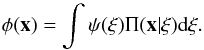 (1)Here ψ is the probability density function (pdf) that represents our prior knowledge about ψ(ξ)dξ, the distribution of probability in ξ-space for the SB1’s true elements.
Since SB1’s with small e’s are of interest, we suppose that Sterne’s (1941) elements have been chosen, as in LS. The six elements are then: P, the orbital period; γ, the systemic velocity; K, the semi-amplitude of the velocity curve; T0, an epoch at which the mean longitude is zero; and the pair ecosω,esinω. In terms of these parameters, the radial velocity curve of an SB1 is given by Eq. (1) in LS.
With this choice and the assumption e2 ≪ 1, the off-diagonal elements of the least-squares matrix have zero expectation values when observational weight is uniformly distributed in phase (LS). Since observers strive to meet this condition, we assume it to be true; and this then implies negligible correlations between the elements. Accordingly, to a good approximation, the error-broadening kernel Π(x | ξ) is simply the product of the six Gaussians giving the independent error distributions of the six elements.
Next consider the pdf ψ(ξ), which is convolved in Eq. (1) with the kernel Π(x | ξ). It follows that ψ is only relevant if it varies significantly within the error bars of an individual orbital element. This is not true for P,γ,K, and T0. However, when orbit circularisation is taken into account, ψ(ξ) may vary significantly within the domain (ecosω ± σecosω,esinω ± σesinω). Accordingly, we now integrate Eq. (1) with respect to the (P,γ,K,T0)-components of x and use the normalization of Π(x | ξ)dx with respect to each of these four elements. The result is 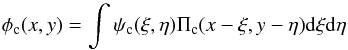 (2)where x = ecosω and y = esinω are the two surviving estimated quantities, whose error-free values are ξ = εcosϖ and η = εsinϖ, respectively, and the subscript c indicates that the pdf’s are defined on a Cartesian grid.
We now assume that the standard errors of ecosω and esinω are equal, which is true of their expectation values when observational weight is uniformly distributed in phase (LS). The broadening kernel is then the circular normal distribution ![Mathematical equation: \begin{equation} \Pi_{\rm c}(x-\xi,y-\eta) = \frac{1}{2 \pi \mu^{2}} \exp \left[-\frac{(x-\xi)^{2}+(y-\eta)^{2}}{2 \mu^{2}} \right] \end{equation}](/articles/aa/full_html/2013/03/aa19819-12/aa19819-12-eq48.png) (3)where μ = σecosω = σesinω.
(3)where μ = σecosω = σesinω.
Bayes’ theorem can now be invoked to derive – see Eq. (10) in L74 – the posterior probability 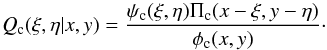 (4)Thus, if the least-square solution is
  (5)the distribution of probability in (εcosϖ,εsinϖ)-space is given by Qc(ξ,η | x,y)dξdη. To evaluate this posterior distribution, we must specify what our expectations were for ψc(ξ,η)dξdη, the prior distribution of probability in (εcosϖ,εsinϖ)-space.
For the problem at hand, polar (p) coordinates (ε,ϖ) are more convenient than the Cartesian coordinates (ξ,η) in the above formulae. The Jacobian of the transformation is J = ε, so that, by conservation of probability, 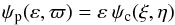 (6)and
  (7)
(7)
2.2. A physical model for ψp
Given P, there is a 2D family of binaries that match the measured K at some inclination. For simplicity, a representative example is chosen to avoid integrating over all possibilities.
Now consider an ensemble of such binaries that form at a uniform rate in the solar neighbourhood and have lifetime t∗. We further suppose that all have ε = ε0 at t = 0 and that thereafter ε decays exponentially with fixed e-folding time t∗/ν, so that  (8)It follows that lnε is uniformly distributed in the interval (lnε∗,lnε0), where ε∗ = ε0exp( − ν). The probability that ε ∈ (ε,ε + dε) is therefore dε/νε.
If we now assume randomly oriented orbits, the probability that ϖ ∈ (ϖ,ϖ + dϖ) is dϖ/2π. Accordingly, the prior probability that a binary is in the element dεdϖ at (ε,ϖ) is ψpdεdϖ, where  (9)Note that ψp decreases with increasing ν = ln (ε0/ε∗). Nevertheless, normalization of this pdf is maintained by the corresponding decrease in ε∗, the lower limit for integrations over ε.
In introducing this physical model, we in effect adopt an informative prior. The following quote is apt: “The real power of Bayesian inference lies in its ability to incorporate “informative” prior information, not “ignorance”” (Feldman & Cousins 1998).
2.3. Distribition of ε
For numerical calculations, it is convenient to transform the integral in Eq. (2) into an integration with respect to the polar coordinates ε and ϖ, so that  (10)and to use logarithmic spacing in ε in order to accurately evaluate the contribution near ε∗. Note that φc is independent of ω when ψp is independent of ϖ, as in Eq. (9).
With φc evaluated, the distribution of probability in (ε,ϖ)-space is given by Qp(ε,ϖ | x,y)dεdϖ, with Qp = εQc from Eq. (4). This 2D pdf, which in general is not independent of ϖ, may be of interest when analysing a particular SB1. But here our interest is in ε, so we integrate over ϖ to obtain 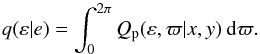 (11)Note that q(ε | e) is independent of ω because of the absence of a correlation term in Πc – see Eq. (3). This in turn follows from the assumptions (Sect. 2.1) that e2 ≪ 1 and that observational weight is uniformly distributed in phase.
The posterior probability that the true eccentricity ∈ (ε,ε + dε) is therefore q(ε | e)dε, with mean value 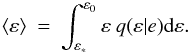 (12)
(12)
2.4. Bayesian terminology
In the above, notation and terminology is from L74. To modern Bayesians, Πc(x − ξ,y − η) is the likelihood and φc(x,y) is the Bayes’ factor. Elsewhere, modern usage is followed with respect to the terms prior pdf, posterior pdf and credible intervals.
3. Numerical results
The theory of Sect. 2 is now illustrated by computing a particular case in detail.
3.1. Parameters
There are two basic parameters, e/μ and ν, the number of e-folding decay times in t∗.
Note that ϵ0 is not a consequential parameter provided that e ≪ ϵ0. In effect, we assume that an SB1 with e ≈ 0 has reached this configuration due to secular evolution and not due to the formation mechanism. In these calculations, ϵ0 = 0.5.
We choose ν = 8.52, so that ε∗ = 10-4. Then, with μ = 0.01, ε(t) < 2.45μ, the LS threshold, when t > 0.35t∗. Thus, from our ensemble of SB1’s, ≈65% would be assigned ε = 0 by the LS test.
3.2. The posterior pdf χ(log ε |e)
Because of the concentration of probability towards ε∗, plots are more informative if the abscissa is log ε rather than ε. Accordingly, we define  (13)In Fig. 1, this pdf is plotted for e/μ = 1.0,2.45,3.03 and 3.72, values selected as follows: if ε = 0, LS showed that the probability pe of exceeding e is given by
  (14)provided that μ ≪ 1. Therefore, when testing H0, the above values of e/μ correspond to levels of significance 61, 5, 1 and 0.1%, respectively. The criterion e/μ > 1 was proposed and implemented by Luyten (1936); the 5% level by LS.
For e/μ = 3.72, χ is an asymmetric bell-shaped function peaking at ≈e, but with a tail extending down to log ε∗ = −4.0. As e/μ decreases, the peak weakens and the tail strengthens. At e/μ = 1.0, the peak is absent and all the probability is in the tail, which derives from the physical model. Intermediate calculations show that the peak first appears at e/μ = 1.42. Thus, for e/μ < 1.42, χ is a monotonically decreasing function of ε. For e/μ > 1.42, χ is unimodal.
The pdf χ for e/μ = 3.72 and μ = 0.01 in Fig. 1 is computed with ε0/μ = 50. Repeating this calculation shows that χ is independent of the upper limit ε0 provided that ε0/μ ≳ 10.
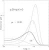 |
Fig. 1 The pdf χ(log ε | e) for the values of e indicated by the vertical lines. These are at e/μ = 1.00,2.45,3.03 and 3.72, corresponding to levels of significance of 61, 5, 1, and 0.1%, respectively. The bold curve is the pdf at the point where the LS-test switches from accepting to rejecting a circular orbit. |
3.3. Percentiles
The posterior pdf’s in Fig. 1 imply asymmetric and rapidly changing credible (or Bayesian confidence) intervals as e/μ varies. These are plotted in Fig. 2 for the indicated values of the probability that the true eccentricity is <ε. For the normal distribution, the values 0.159,0.500,0.841 and 0.977 correspond to displacements of − 1,0, + 1 and + 2σ, respectively.
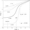 |
Fig. 2 Credible intervals for the posterior pdf χ(log ε | e) as functions of e. The plotted boundaries correspond to the true eccentricity being <ε with the indicated probabilities. The values of e corresponding to levels of significance 61% (Luyten) and 5% (LS) are indicated, as is the regime transition at e†. |
Figure 2 reveals a dramatic switch in solution regime at e†/μ ≈ 3.6. For e ≳ e†, the measured value e is close to the 50% percentile and is tightly enclosed by the ±1σ intervals. In this regime, inferences are dominated by the actual measurement e ± μ. But this ceases to be so for e ≲ e†. Thus, for e/μ < 2.65, the “solution” ε = e falls outside the ± 1σ intervals. Evidently, for e ≲ e†, inferences are increasingly dominated by the model of Sect. 2.2.
3.4. Highest posterior density intervals
For e/μ < 1.42, χ is a monotonically decreasing function of ε (Sect. 3.2). It follows that traditional, equal-tail credible intervals exclude the point (ε = ε∗) with greatest probability density (pd). This undesirable feature is avoided by instead computing highest posterior density intervals (HPDI; Box & Tiao 1973). These intervals are such that every point included has a higher pd than every point excluded.
In general, the calculation of HPDIs is non-trivial. But here the pdf’s χ are not pathological (Fig. 1), and so the following clipping algorithm finds the HPDI for specified e and designated enclosed probability (1 − α).
Let log εkL,...,log εkU be consecutive grid points that belong to and define the HPDI (εkL,εkU). Then an HPDI with smaller included probability is obtained by eliminating the grid point log εkL if χkL < χkU or the grid point log εkU if χkU < χkL. This is repeated until the included probability = (1 − α).
The 95% HPDIs thus obtained for χ(log ε | e) are plotted for e = 0.000(0.001)0.080 in Fig. 3. For e < 0.018, the HPDIs are effectively one-tail intervals since the lower bound is εL = ε∗ = 10-4. Accordingly, for this problem, HPDIs provide a seamless transition from upper limits for non-detected to two-sided intervals for detected eccentricities (cf. Feldman & Cousins 1998). This is an appealing aspect of HDPIs for interpreting measured e’s and their uncertainties.
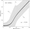 |
Fig. 3 Highest posterior density intervals for the posterior pdf χ(log ε | e). The enclosed posterior probability of each HPDI is 95%, and the prior pdf ψ is given by Eq. (9). The filled circles are the posterior means ⟨ ε ⟩ computed from Eq. (12). |
For e < 0.0142, the interval excluded from an HPDI is a single-tail because of the aforementioned monotonicity. For e > 0.0142, the pdf χ is unimodal (Fig. 1), with a maximum whose location → e as e/μ increases. This emerging, measurement-driven maximum eventually brings about the transition from one- to two-tailed intervals. For e > 0.018, the excluded probability is contained in two tails, with the upper tail’s probability being initially 5%, but this decreases to ≈2.5% when e/μ ≫ 1 because of χ’s increasing symmetry – see Fig. 1.
Note that for the normal distribution,  , the 95% HPDI is the familiar equal tail interval (− 1.96, + 1.96) and the width of this interval is the narrowest that ecloses 95% of the probability. For non-symmetric pdf’s, HPDIs are the narrowest intervals enclosing probability (1 − α) and as such are a natural generalization of the conventional equal-tail intervals for symmetric, bell-shaped pdf’s.
Confidence intervals are an economical means of conveying the compactness or otherwise of a variate’s distribution. The resulting loss of information, if of concern, can be avoided by plotting the pdf’s, as in Figs. 1 and A.2.
3.5. Detection threshold
The transition from one- to two-tailed HPDIs is a natural definition of the detection threshold eth for non-zero eccentricity – i.e., the measured value e above which attribution purely to measurement errors is implausible. However, Fig. 3 shows that εL remains ≪e for a considerable interval beyond eth = 0.018, which in any case depends on ν, a parameter likely to be only crudely estimated.
If detection is crucial for a subsequent investigation – e.g., an observing program – then a threshold closer to e† should be adopted (Figs. 2 and 3).
 |
Fig. 4 Ensemble simulation comprising N = 1000 SB1’s with the parameters of Sect. 3.1. The plotted points randomly sample the time interval (0,t∗), have true eccentricities ε from Eq. (8), and have Gaussian measurement errors added to derive e. The 95% HPDIs (εL,εU) are indicated. For e < eth = 0.018, the lower limit εL = ε∗ = 10-4. |
3.6. Simulation
The role that HPDIs can play in reporting eccentricities is best illustrated by sampling experiments. Accordingly, synthetic data for the model of Sect. 2.2 are created as follows: if z1,z2 are random numbers in (0,1), a random ensemble member in (ε,ϖ)-space is at  (15)Then, if ζ1,ζ2 are random Gaussian variates, this ensemble member is observed at the point
  (16)Repeated N times, the resulting e’s comprise a simulated observing campaign of N random ensemble members whose exact eccentricities ε are known.
With ε∗ = 10-4, a sample of N = 1000 SB1’s are plotted in Fig. 4. As expected, the large majority of the points fall within the 95% HPDIs (εL,εU). With Luyten’s criterion e > μ, 79.5% of this sample would have their elliptical orbits accepted. But Fig. 4 clearly shows that most systems with e ∈ (0.01,0.03) have ε < 0.01 and so exceed Luyten’s criterion because of the bias of the non-negative estimator e (LS). With the LS criterion e > 2.45μ, the accepted percentage drops to 40.5, and most of the systems with e ∈ (0.01,0.03) would now be assigned ε = 0, a marked improvement.
The further improvement provided by the HPDIs is that the assignment ε = 0 can now be replaced by an upper limit. Thus, for example, with this choice of prior, an SB1 with e = 0.01 ± 0.01 is preferably reported as ε < ε95 = 0.014. From the standpoint of testing theories of tidal dissipation, an upper limit is more informative than ε = 0.
The sampling procedure can also be used to validate the upper limits. A sample with N = 106 has 161, 521 systems with log e ∈ (−2.1, −1.9) and 8,317 of these have ε > ε95. Thus 94.85% lie below the upper limit, closely agreeing with the designated 95%.
3.7. Upper limits
Upper limits εU when e < eth are the most useful products of this Bayesian machinery. With their validity confirmed above, their dependence on the orbital decay rate is now explored.
Consider the representative measurement e = 0.01 ± 0.01, so that e/μ = 1.0, well below the detection threshold. In Table 1, the HPDI 95% upper limits ε95 are given for this e/μ as a function of ε∗. The decrease of ε95 with increasing ν reflects statistical reality: if the e-folding time t∗/ν ≪ t∗, most systems will have ε ≪ e and a correspondingly small ε95. Note that ε95 even drops below e when ν ≳ 13.
In analysing an observed system without a good estimate of ν or, equivalently, of ε∗, the conservative approach is to suppose that ε∗ is no more than a factor ~10 below the measured e, thus avoiding claiming too low an upper limit εU. An even more conservative approach is to adopt a uniform prior – see Appendix.
HPDI 95% upper limits ε95 when e/μ = 1.0.
4. Conclusion
In this paper, by incorporating a model of an SB1’s secular evolution, Bayes’ theorem is used to infer bounds on its exact eccentricity ε given its measured value e ± μ. Because the system’s lifetime t∗ is finite, the asymptote ε = 0 is never reached. Thus, in contrast to Luyten (1936) and LS, the statistical problem is not one of model selection. Systems assigned ε = 0 by these earlier tests should preferably have upper limits εU computed.
As Fig. 4 shows, the Bayesian upper limits contain the systems for which e is significantly larger than ε due to measurement errors and bias. Thus, a major historical cause of spurious e’s is eliminated. But physical causes remain, such as those due to proximity effects or to additional line absorption by gas streams. An example is ζ TrA, for which Skuljan et al. (2004) improved the precision of the radial velocities by a remarkable factor of 100 and reported a small but highly significant e = 0.0140 ± 0.0002. However, the significant non-detection of the Keplerian third harmonic (Lucy 2005) invalidated this claim1. As precision improves, similar testing for the third and higher Keplerian harmonics is essential for confirming that an orbit is truly eccentric. In addition, an update of Savedoff’s (1951) work would provide numerous examples of spurious e’s for investigation into physical causes other than measurement bias.
Hearnshaw et al. (2012) have just reported eleven additional non-detections.
Acknowledgments
I am grateful to the referee for pointing out an error in statistical terminology.
References
- Box, G. E. P., & Tiao, G. C. 1973, Bayesian Inference in Statistical Analysis, (Reading MA: Addison-Wesley) [Google Scholar]
- Eastman, J., Gaudi, B. S., & Agol, E. 2013, PASP, 125, 83 [NASA ADS] [CrossRef] [Google Scholar]
- Feldman, G. J., & Cousins, R. D. 1998, Phys. Rev. D, 57, 3873 [Google Scholar]
- Ford, E. B. 2006, ApJ, 642, 505 [NASA ADS] [CrossRef] [Google Scholar]
- Hearnshaw, J. B., Komonjinda, S., Skuljan, J., & Kilmartin, P. M. 2012, MNRAS, 427, 298 [NASA ADS] [CrossRef] [Google Scholar]
- Lucy, L. B. 1974, AJ, 79, 745 (L74) [NASA ADS] [CrossRef] [Google Scholar]
- Lucy, L. B. 2005, A&A, 439, 663 [NASA ADS] [CrossRef] [EDP Sciences] [Google Scholar]
- Lucy, L. B., & Sweeney, M. A. 1971, AJ, 76, 544 (LS) [NASA ADS] [CrossRef] [Google Scholar]
- Luyten, W. J. 1936, ApJ, 84, 85 [NASA ADS] [CrossRef] [Google Scholar]
- Savedoff, M. P. 1951, AJ, 56, 1 [NASA ADS] [CrossRef] [Google Scholar]
- Skuljan, J., Ramm, D. J., & Hearnshaw, J. B. 2004, MNRAS, 352, 975 [NASA ADS] [CrossRef] [Google Scholar]
- Sterne, T. E. 1941, Proc. Natl. Acad. Sci. U.S., 27, 175 [NASA ADS] [CrossRef] [Google Scholar]
Appendix A: Uniform prior
The model of Sect. 2.2 is not appropriate if the SB or star-planet system has additional components causing significant gravitational perturbations. In this circumstance, a sensible option is to assume a uniform prior for ε, as is already common practice for exoplanets (e.g., Ford 2006; Eastman et al. 2013). Together with the assumption of randomly oriented orbits, the prior probability of the system being in dεdϖ is then ψpdεdϖ, where 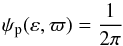 (A.1)which now replaces Eq. (9) in Sects. 2.3 and 3.
From the resulting posterior pdf q(ε | e), the 95% HPDIs and means ⟨ ε ⟩ are plotted in Fig. A.1 for e ∈ (0.00,0.08). Comparison with Fig. 3 shows that the HPDIs are nearly identical for e/μ ≳ 5. However, for e/μ ≲ 2 – i.e., in the non-detection domain – the upper limits εU in Fig. 3 are markedly lower, reflecting the effect of tidal circularisation in creating systems with ε ≪ e.
In contrast with Fig. 3, Fig. A.1 shows that a uniform prior results in a sharply defined detection threshold eth/μ = 2.49, which is gratifyingly close to the (frequentist) LS value eLS/μ = 2.45 given by Eq. (14) for pe = 0.05. The thresholds for other critical levels are given in Table A.1, with the corresponding upper limits (bounds) εU in Table A.2.
For the representative measurement e/μ = 1.0 of Sect. 3.7, the 95% upper limit from Table A.2 is 2.41μ. This exceeds the corresponding values in Table 1, confirming that the uniform prior is the more conservative option.
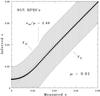 |
Fig. A.1 Highest posterior density intervals for the posterior pdf q(ε | e). The enclosed posterior probability of each HPDI is 95%, and the prior pdf ψ is given by Eq. (A.1). The filled circles are the posterior means ⟨ ε ⟩ computed from Eq. (12). |
 |
Fig. A.2 Detection threshold. The posterior pdf q(ε | e) for eth = 0.0249, the measured value for marginal detection (Sect. 3.5). The hatched area with ε > εU = 0.0394 contains 5% of the probability. Note that q(0 | eth) = q(εU | eth). |
Detection thresholds for e.
Upper limits (bounds) for ε.
A.1: A revised Lucy-Sweeney test
Even without evidence of additional components, an investigator may be reluctant to base an analysis of orbital elements on uncertain estimates of tidal decay. If so, the assumption of a uniform prior for ε should be attractive. Physically, this corresponds to no secular evolution of εand a formation mechanism that uniformly populates the interval 0 < ε < 1. Accordingly, a system with e ≈ 0 is assumed to have formed as such (cf. Sect. 3.1).
This neutral standpoint is an attractive basis for a revised version of the LS test in which the previous acceptance of a circular orbit (H0) is now replaced by an upper limit.
The revised LS test with 1 − α = 0.95 proceeds as follows:
1): The eccentricitye ± μ is derived from the least squares solution.
2): If e/μ > 2.49, this measured value e ± μ is accepted.
3): However, if e/μ < 2.49, the measured value is replaced by the upper limit ε95 obtained by interpolation in Col. 4 of Table A.2.
To illustrate this revised test, upper limits are given in Table A.3 for six SB1’s for which circular orbits are reported on the first page of Table 1 in LS. Thus for YZ Cas, the least squares value e = 0.004 was rejected by the LS test and ε = 0 accepted. We now compute the 95% upper limit as follows: the estimate μ = 0.0037 is derived from Eq. (13) and Table 1 of LS. Linear interpolation in Table A.2 at e/μ = 1.1 then gives ε95/μ = 2.50, whence ε < ε95 = 0.009. Table A.3. shows that upper limits can differ by large factors, reinforcing the earlier remark (Sect. 3.6) that upper limits are to be preferred in testing theories of tidal dissipation. A critical data base of detections and upper limits would facilitate progress in this field.
Upper limits ε95 for SB1 sample.
All Tables
All Figures
|
Fig. 1 The pdf χ(log ε | e) for the values of e indicated by the vertical lines. These are at e/μ = 1.00,2.45,3.03 and 3.72, corresponding to levels of significance of 61, 5, 1, and 0.1%, respectively. The bold curve is the pdf at the point where the LS-test switches from accepting to rejecting a circular orbit. |
| In the text | |
|
Fig. 2 Credible intervals for the posterior pdf χ(log ε | e) as functions of e. The plotted boundaries correspond to the true eccentricity being <ε with the indicated probabilities. The values of e corresponding to levels of significance 61% (Luyten) and 5% (LS) are indicated, as is the regime transition at e†. |
| In the text | |
|
Fig. 3 Highest posterior density intervals for the posterior pdf χ(log ε | e). The enclosed posterior probability of each HPDI is 95%, and the prior pdf ψ is given by Eq. (9). The filled circles are the posterior means ⟨ ε ⟩ computed from Eq. (12). |
| In the text | |
|
Fig. 4 Ensemble simulation comprising N = 1000 SB1’s with the parameters of Sect. 3.1. The plotted points randomly sample the time interval (0,t∗), have true eccentricities ε from Eq. (8), and have Gaussian measurement errors added to derive e. The 95% HPDIs (εL,εU) are indicated. For e < eth = 0.018, the lower limit εL = ε∗ = 10-4. |
| In the text | |
|
Fig. A.1 Highest posterior density intervals for the posterior pdf q(ε | e). The enclosed posterior probability of each HPDI is 95%, and the prior pdf ψ is given by Eq. (A.1). The filled circles are the posterior means ⟨ ε ⟩ computed from Eq. (12). |
| In the text | |
|
Fig. A.2 Detection threshold. The posterior pdf q(ε | e) for eth = 0.0249, the measured value for marginal detection (Sect. 3.5). The hatched area with ε > εU = 0.0394 contains 5% of the probability. Note that q(0 | eth) = q(εU | eth). |
| In the text | |
Current usage metrics show cumulative count of Article Views (full-text article views including HTML views, PDF and ePub downloads, according to the available data) and Abstracts Views on Vision4Press platform.
Data correspond to usage on the plateform after 2015. The current usage metrics is available 48-96 hours after online publication and is updated daily on week days.
Initial download of the metrics may take a while.