| Issue |
A&A
Volume 548, December 2012
|
|
|---|---|---|
| Article Number | A4 | |
| Number of page(s) | 34 | |
| Section | Extragalactic astronomy | |
| DOI | https://doi.org/10.1051/0004-6361/201219368 | |
| Published online | 13 November 2012 | |
Millimeter imaging of submillimeter galaxies in the COSMOS field: redshift distribution⋆,⋆⋆
1
ESO ALMA COFUND Fellow
2
European Southern Observatory, Karl-Schwarzschild-Strasse 2, 85748
Garching,
Germany
e-mail: This email address is being protected from spambots. You need JavaScript enabled to view it.
3 Argelander-Institute for Astronomy, Auf dem Hügel 71, Bonn,
53121, Germany
4
University of Zagreb, Physics Department,
Bijenička cesta 32,
10002
Zagreb,
Croatia
5
European Southern Observatory, Alonso de Córdoba 3107, Vitacura, Casilla 19001,
Santiago 19,
Chile
6
Max-Planck-Institut für Radioastronomie,
Auf dem Hügel 69, 53121
Bonn,
Germany
7
Max Planck Institute for Astronomy, Königstuhl 17, 69117
Heidelberg,
Germany
8
California Institute of Technology, MC 249-17, 1200 East California Boulevard,
Pasadena, CA
91125,
USA
9
IRAM, 300 rue de la piscine, 38406 Saint-Martin
d’Hères,
France
10
Max-Planck-Institut für Extraterrestrische Physik,
Giessenbachstraße, 85748
Garching,
Germany
11
Laboratoire AIM-Paris-Saclay, CEA/DSM/Irfu CNRS Université Paris
Diderot, CE-Saclay, pt courrier
131, 91191
Gif-sur-Yvette,
France
12
Institut d’Astrophysique de Paris, UMR 7095 CNRS, Université
Pierre et Marie Curie, 98bis
boulevard Arago, 75014
Paris,
France
13
National Radio Astronomy Observatory, PO Box 0, Socorro, NM
87801-0387,
USA
14
INAF – Osservatorio Astronomico di Bologna, via Ranzani
1, 40127
Bologna,
Italy
15
Harvard-Smithsonian Centre for Astrophysics, 60 Garden
Street, Cambridge,
MA
02138,
USA
16
Laboratoire d’Astrophysique de Marseille, Université de Provence,
CNRS, BP 8,
Traverse du Siphon,
13376
Marseille Cedex 12,
France
17
National Optical Astronomy Observatory,
950 North Cherry Avenue,
Tucson, AZ
85719,
USA
18
Institute for Astronomy, ETH Zürich, Wolfgang-Pauli-strasse 27,
8093
Zürich,
Switzerland
19
Institute for Astronomy, University of Hawaii,
2680 Woodlawn Drive,
Honolulu, HI, 96822, USA
20
National Radio Astronomy Observatory, 520 Edgemont Road, Charlottesville, VA
22903,
USA
21
Research Center for Space and Cosmic Evolution, Ehime
University, Bunkyo-cho, Matsuyama
790-8577,
Japan
Received: 8 April 2012
Accepted: 24 May 2012
Abstract
We present new IRAM Plateau de Bure interferometer (PdBI) 1.3 mm continuum observations at ~1.5′′ resolution of 28 submillimeter galaxies (SMGs), previously discovered with the 870 μm bolometer LABOCA at the APEX telescope from the central 0.7 deg2 of the COSMOS field. Nineteen out of the 28 LABOCA sources were detected with PdBI at a ≳3σ level of ≈1.4 mJy/beam. A combined analysis of this new sample with existing interferometrically identified SMGs in the COSMOS field yields the following results: i) ≳15%, and possibly up to ~40% of single-dish detected SMGs consist of multiple sources; ii) statistical analysis of multi-wavelength counterparts to single-dish SMGs shows that only ~50% have real radio or IR counterparts; iii) ~18% of interferometric SMGs have either no multi-wavelength counterpart or only a radio-counterpart; and iv) ~50–70% of z ≳ 3 SMGs have no radio counterparts (down to an rms of 7–12 μJy at 1.4 GHz). Using the exactinterferometric positions to identify the multi-wavelength counterparts allows us to determine accurate photometric redshifts for these sources. The redshift distributions of the combined and the individual 1.1 mm and 870 μm selected samples shows a higher mean and a broader width than those derived in previous studies. This study finds that on average brighter and/or mm- selected SMGs are located at higher redshifts, consistent with previous studies. The mean redshift for the 1.1 mm selected sample ( = 3.1 ± 0.4) is tentatively higher than that for the 870 μm selected sample ( = 2.6 ± 0.4). Based on our nearly complete sample of AzTEC 1.1 mm SMGs in a 0.15 deg2 area, we infer a higher surface density of z ≳ 4 SMGs than predicted by current cosmological models. In summary, our findings imply that interferometric identifications at (sub-)millimeter wavelengths are crucial to build statistically complete and unbiased samples of SMGs.
Key words: surveys / galaxies: starburst / galaxies: fundamental parameters / galaxies: high-redshift / galaxies: statistics / submillimeter: galaxies
Based on observations carried out with the IRAM Plateau de Bure Interferometer. IRAM is supported by INSU/CNRS (France), MPG (Germany) and IGN (Spain).
Appendices are available in electronic form at http://www.aanda.org
© ESO, 2012
1. Introduction
1.1. Submillimeter galaxies
Submillimeter galaxies (SMGs; S850 μm ≳ 5 mJy) are ultra-luminous, dusty, starburst galaxies with extreme star formation rates of order 103 M⊙ yr-1 (e.g. Blain et al. 2002). They trace a phase of the most intense stellar mass build-up in galaxies and contribute significantly to the volume-averaged cosmic star formation rate density at z = 2−3 (~20%; Michalowski et al. 2010). Evidence is emerging that SMGs represent the progenitors of massive elliptical galaxies (e.g. Cimatti et al. 2008; van Dokkum et al. 2008; Michalowski et al. 2010), and their enhanced star formation properties may be intimately related to the evolution of quasi stellar objects (Sanders et al. 1996; Hopkins et al. 2006; Hayward et al. 2011).
Spectroscopic and photometric studies of SMGs locate them predominantly at redshifts 2–3 (e.g. Chapman et al. 2005; Wardlow et al. 2011), and only a few z > 4 SMGs have recently been detected. Identifying the highest redshift SMGs requires time-consuming, systematic follow-up observations to properly identify them against strong lower-redshift selection biases. To date ~10 z > 4 SMGs have been confirmed (Daddi et al. 2009a,b; Capak et al. 2008, 2011; Schinnerer et al. 2008; Coppin et al. 2009; Knudsen et al. 2010; Carilli et al. 2010, 2011; Riechers et al. 2010; Smolčić et al. 2011; Cox et al. 2011; Combes et al. 2012).
Although the number of high redshift (z > 4) SMGs remains small it appears that their abundance is so high that it is only marginally consistent with current galaxy formation models (Baugh et al. 2005; Coppin et al. 2009; Smolčić et al. 2011). It has also been suggested that high-redshift SMGs may be qualitatively different from those at intermediate redshift (Wall et al. 2008). However, such conclusions are premature given the significant uncertainties in identification of SMGs with optical/IR sources, and therefore the appropriate measurement of their redshift.
1.2. Identifying multi-wavelength counterparts to SMGs
SMGs are typically first detected with single-dish mm or sub-mm telescopes which have a relatively large (10′′−35′′) beam size which may include tens of galaxies in the visible or NIR. Numerous methods have been applied to pinpoint the proper counterparts, such as UV/IR/radio star formation indicators or an association with AGN (Ivison et al. 2005, 2007; Bertoldi et al. 2007; Biggs et al. 2010). These techniques are problematic because the identification is probabilistic and thus introduces the possibility of sample incompletness, contamination, and/or bias. Moreover SMGs may be tightly clustered and thus blended in single dish observations (e.g., Younger et al. 2007, 2009). Interferometric observations of SMGs at intermediate-resolution (~2′′) shows that they often do not coincide with any galaxy at any wavelength (Younger et al. 2009). This may be due to extreme dust extinction or due to a very high-redshift for the galaxy. To assess the overall properties of SMGs including their redshift distribution, it is therefore crucial to follow up single-dish detections with high resolution interferometric imaging. Before the improved sensitivities provided by the upgraded IRAM PdBI or ALMA, interferometric follow-up at millimeter or submillimeter wavelengths was slow and expensive. Only about 50 SMGs have been properly identified in various survey fields (Downes et al. 1999, Frayer et al. 2000; Dannerbauer et al. 2002; Downes & Solomon 2003; Genzel et al. 2003; Kneib et al. 2005; Greve et al. 2005; Tacconi et al. 2006; Sheth et al. 2004, Iono et al. 2006; Younger et al. 2007, 2009; Aravena et al. 2010a; Ikarashi et al. 2011; Tamura et al. 2010; Hatsukade et al. 2010; Wang et al. 2011; Chen et al. 2011; Neri et al. 2003; Chapman et al. 2008; Smolčić et al. 2012). The largest statistically significant, signal-to-noise- and flux-limited sample of interferometrically identified SMGs contains 17 sources drawn from the AzTEC/JCMT survey of 0.15Λ° within the COSMOS field (Younger et al. 2007, 2009). Here we present PdBI observations towards 28 SMGs drawn from the LABOCA-COSMOS 0.7Λ° survey (Navarrete et al., in prep.), which constitutes the largest interferometric follow-up of SMGs drawn from bolometer imaging surveys to date.
1.3. Determining the redshift of SMGs
The proper identification with an optical counterpart may allow a determination of the SMG redshift through deep optical/NIR spectroscopy. Given the ambiguity of identifications through probability considerations and the optical faintness of the counterparts, and the absence of lines in particular redshift ranges, this has been a very difficult task. The largest SMG sample with spectroscopic redshifts to date was established by Chapman et al. (2005), who followed-up SMG counterparts identified through deep, intermediate (≲2′′) resolution radio observations, getting redshifts for 76 of 150 targets.
Where spectroscopic redshifts cannot be measured for large samples of SMGs, deep panchromatic surveys such as COSMOS or GOODS can measure photometric redshifts, which are based on χ2 minimization fits of multi-band photometry to spectral models (e.g. Ilbert et al. 2009). With an optimized choice of spectral models and dense multi-wavelength photometric coverage photometric redshifts can reach accuracies of a few percent (e.g. Ilbert et al. 2009). Although it was not obvious whether common photometric redshift templates could be applied to SMG counterparts, recent studies confirm that photometric redshifts can be estimated for SMGs, both on statistical and a case by case basis (e.g. Daddi et al. 2009a; Wardlow et al. 2010, 2011; Yun et al. 2012; Smolčić et al. 2012). Here we further test the photometric redshift estimates for SMGs using the largest “training set” of SMGs with secure spectroscopic redshifts to date from COSMOS.
In Sect. 2 we describe the data used for our analysis. In Sect. 3 we present the PdBI observations towards 28 SMGs drawn from the LABOCA-COSMOS survey. In Sect. 4 we define two samples of SMGs with mm-interferometric detections in the COSMOS field. Using these in Sect. 5 we investigate blending of SMGs, and usually applied statistical counterpart association methods to single-dish identified SMGs. In Sect. 6 we calibrate photometric redshifts for SMGs. In Sect. 7 we derive redshift distributions for our statistical samples of SMGs with unambiguously determined counterparts. We discuss and summarize our results in Sects. 8 and 9. We adopt H0 = 70 km s-1 Mpc-1, ΩM = 0.3, ΩΛ = 0.7, and use a dust emissivity index of β = 1, and a Chabrier (2003) initial-mass function if not stated otherwise.
Summary of interferometrically observed COSMOS SMGs besides our work.
LABOCA sources observed with the PdBI.
2. Data
2.1. The COSMOS Project
The Cosmic Evolution Survey (COSMOS) is an imaging and spectroscopic survey of an equatorial 2Λ° field (Scoville et al. 2007). The field has been observed with most major space- and ground-based telescopes over most of the electromagnetic spectrum. The COSMOS Project has obtained very deep broad-band (u * BVgrizJHK) and medium and narrow-band imaging data in over 30 optical to near-infrared bands. Additionally, there is GALEX, Spitzer IRAC/MIPS, Herschel PACS/SPIRE, HST/ACS, XMM-Newton, VLA (1.4 GHz and 320 MHz), GMRT (600 & 200 MHz) data, as well over 25,000 optical spectra (Capak et al. 2007; Sanders et al. 2007; Scoville et al. 2007; Leauthaud et al. 2007; Koekemoer et al. 2009; Frayer et al. 2009; Hasinger et al. 2007; Zamojski et al. 2007; Taniguchi et al. 2007; Lilly et al. 2007, 2009; Le Floc’h et al. 2009; McCracken et al. 2010; Trump et al. 2007; Schinnerer et al. 2004, 2007, 2010; Smolčić et al., in prep.). The inner square degree of COSMOS has also been observed in X-rays at a higher resolution and sensitivity with Chandra (Elvis et al. 2009) and at mm and submm wavelengths with AzTEC, BOLOCAM, MAMBO and LABOCA (Aretxaga et al. 2010; Navarrete et al., in prep.; Bertoldi et al. 2007, Aguirre et al., in prep., Scott et al. 2008).
Particularly relevant for the work presented here are the deep UltraVista observations of COSMOS which reach 5σ (2′′ aperture AB magnitude) sensitivities of 24.6, 24.7, 23.9, and 23.7 in Y, J, H, and Ks bands respectively (McCracken et al. 2012), as well as the VLA 1.4 GHz observations which reach a rms of 7–12 μJy/beam (Schinnerer et al. 2004, 2007, 2010). We use the updated UV-MIR COSMOS photometric catalog (Capak et al. 2007) including all available UV-MIR photometric observations.
2.2. Submillimeter galaxies in the COSMOS field
The COSMOS field was mapped at mm or submm wavelengths with MAMBO at the IRAM 30 m (0.11 deg2; 1.2 mm, 11′′ angular resolution; Bertoldi et al. 2007), BOLOCAM at the CSO (0.27 deg2; 1.1 mm; 31′′ angular resolution; Aguirre et al., in prep.), AzTEC at the JCMT (0.15 deg2; 1.1 mm; 18′′ angular resolution; Scott et al. 2008), AzTEC at ASTE (0.72 deg2; 1.1 mm; 34′′ angular resolution; Aretxaga et al. 2011), and LABOCA at APEX (0.7 deg2; 870 μm; 27′′ angular resolution, Navarette et al., in prep.). To properly determine the multi-wavelength counterparts of the SMGs identified in these surveys, numerous interferometric and spectroscopic follow-up efforts have been made (Younger et al. 2007, 2008, 2009; Capak et al. 2008, 2010; Schinnerer et al. 2008; Riechers et al. 2010; Aravena et al. 2010a; Smolčić et al. 2011, 2012; Karim et al. 2012, in prep.). To date a sample of 24 interferometrically identified COSMOS SMGs has been established prior to our observations (Table 1). For 11 of those spectroscopic redshifts are available, either from a dedicated COSMOS optical spectroscopic follow-up campaign using Keck II/DEIMOS (Capak et al., in prep.; Karim et al., in prep.), or from CO line observations with mm interferometers (Schinnerer et al. 2008; Riechers et al. 2010, in prep.; Baloković et al., in prep.; Karim et al., in prep.; Sheth et al., in prep.).
3. PdBI follow-up of LABOCA-COSMOS SMGs
PdBI detections.
3.1. Observations
The COSMOS-LABOCA observations1 reach a rms of 1.5 mJy per beam (27.6′′). The rms increases towards the edges of the map, and the catalog was extracted from an area of ~0.7 deg2 (Navarrete et al., in prep.). Our sample of 28 COSMOS LABOCA sources selected for PdBI follow-up observations (Table 2) was chosen with a requirement that the signal-to-noise in the LABOCA map is S/N870 μm ≳ 3.8. Eight other LABOCA-COSMOS sources had already been observed previously with mm-interferometers2 (see Table 1).
The SMGs in our sample were observed using the PdBI during two nights in Oct./Nov. 2007 (COSLA-10, and COSLA-19) and three nights in Oct./Nov. 2011 (the remaining 26 SMGs) in C- and D-configurations with 6 working antennas and the updated PdBI system. All observations were done in good/excellent millimeter weather conditions. During our 2007 observations we used the full 2 GHz bandwidth available with the correlator at the PdBI, and the receivers were tuned to 232 GHz and 231.5 GHz for observations of COSLA-19 and COSLA-10, respectively. The total on-source time was 2.3 and 2.2 h for COSLA-10, and COSLA-19, respectively. Our 2011 observations were done using the WideX correlator covering a bandwidth of 3.6 GHz, with receivers tuned to 230 GHz (1.3 mm). These observations were performed in snap-shot mode cycling through the 26 SMGs in each track and observing the phase/amplitude calibrator for 2.25 min every 19.5 min. The total on-source time reached is ~43 min per source.
Sources J1055+018, J1005+066, J0923+392 were used for phase/amplitude calibration, and MWC349, J0923+392, 3C84 for flux calibration which we consider accurate within 10–20%. Calibration and editing was done using the GILDAS CLIC package. For each source, the final uv data were collapsed in frequency. The final dirty maps reach an rms noise level of 0.55 mJy beam-1 and 0.39 mJy beam-1, with FWHM beam sizes of 3.3′′ × 2.3′′ and 3.0′′ × 2.1′′ for COSLA-19 and COSLA-10, respectively, and an rms of 0.46 mJy beam-1 with FWHM ~ 1.8′′ × 1.1′′ for the remaining SMGs.
3.2. PdBI mm-sources
We searched for point sources in the dirty 1.3 mm PdBI maps within a ~14′′ radius from the phase center, which about corresponds to the LABOCA map resolution of 27′′. Peaks with S/N > 4.5 were considered detections regardless of any multi-wavelength association. When such peaks were present in sidelobe-contaminated regions, we tested the reality of the sources by cleaning the map by setting a CLEAN box around the brightest peak (see Appendix A for notes on individual sources). For peaks with 3 ≲ S/N ≤ 4.5 we required an associated optical, near/mid-IR, or radio source within a radius of ≲1′′. Assuming a Gaussian noise distribution, the S/N > 4.5 requirement implies a false detection rate of ~0.15% within a search radius of 14′′. A mm source association with optical, NIR, MIR, or radio sources further decreases the probability that the source is false3. Given the surface densities of sources present in various catalogs the false match probabilities independently estimated for each band are 12% (optical), ~2% (for each, UltraVista Y, J, H, Ks, and IRAC 3.6 μm), and 0.017% (20 cm radio).
To further constrain the false match probability, we performed a source search in the same way as described above, but on the inverted, i.e. negative maps. We find only one occurrence of a >4.5σ (i.e. 4.8σ) peak (~10′′ away from the phase center and with no multi-wavelength counterpart) consistent with the above given false match probability expectation. We further find ~10% of 3 ≲ S/N ≤ 4.5 peaks matched to multi-wavelength counterparts. This suggests a ~10% false match probability for our 3 ≲ S/N ≤ 4.5 sources. Hereafter we consider S/N > 4.5 detections as significant and those with 3 < S/N ≤ 4.5 as tentative.
The 1.3 mm sources and their properties are summarized in Table 3. Comments on individual sources and their PdBI maps and multi-wavelength stamps are presented in Appendix A. Of the 28 LABOCA sources observed, 9 yielded no detection in the 1.3 mm maps (see next section). Six of the 19 detected LABOCA sources break up into multiple sources, so that in total we identify 26 submm sources. Nine of these 26 sources have S/N > 4.5, 7 have S/N between 4 and 4.5, and 10 between 3 and 4. The distribution of separations between the LABOCA source position and the corresponding PdBI source position is shown in Fig. 1. We find a median separation of 6.40′′ for all sources, and 5.95′′ for those with S/N870 μm ≥ 3.8. This is consistent with the results based on artificial source tests performed on the LABOCA map. They result in a positional uncertainty for LABOCA sources down to S/N870 μm = 3.8 of ~5.3′′ with an inter-quartile range of 3.1′′−9.8′′ (Navarrete et al., in prep.).
All detections except COSLA-6-1 and COSLA-6-2 are consistent with point-sources at our resolution. We extract their fluxes from the brightest pixel value in the dirty maps. The flux uncertainty is estimated as the rms noise level in the map. The fluxes for COSLA-6-1 and COSLA-6-2 were obtained by fitting a double Gaussian to the source. All fluxes (tabulated in Table 3) were corrected for the primary beam response of the PdBI dishes (assuming a Gaussian distribution with HPBW of 21′′).
Scaling the observed 1.3 mm fluxes to the LABOCA 870 μm, and where available to the AzTEC 1.1 mm, or MAMBO 1.2 mm fluxes (Table 2), yields consistent values4. This is shown in Fig. 2 and described in more detail for each source in Appendix A. This further strengthens the validity of our detections.
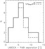 |
Fig. 1 Distribution of separations between the PdBI sources and the corresponding LABOCA-COSMOS sources. |
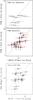 |
Fig. 2 Comparison between LABOCA 870 μm and PdBI 1.3 mm fluxes for SMGs (indicated in the panel) detected (middle panel) and not detected (top panel) with the PdBI. For LABOCA sources identified as multiple PdBI sources the individual PdBI source fluxes were added, and for the LABOCA sources not detected by PdBI 1.3 mm flux estimates for the most likely multi-wavelength counterparts were extracted from the PdBI maps (see Sect. 3.3 for details). The bottom panel shows the comparison between AzTEC 1.1 mm and SMA 890 μm fluxes (adopted from Younger et al. 2007, 2009) for AzTEC/JCMT SMGs in our 1.1 mm-selected sample. The solid line in all panels shows the flux ratios for a spectral power law index of 3. |
3.3. Non-detections
Nine LABOCA sources remain undetected within our PdBI observations. The reasons for this could be that i) the LABOCA sources are fainter than our PdBI sensitivity limit (1σ ~ 0.46 mJy), ii) the LABOCA sources break up into multiple components at 1.5′′ resolution and are all fainter than our flux limit or iii) the LABOCA source is spurious. To investigate this further we have made use of the COSMOS multi-wavelength data by assigning statistical counterparts to those LABOCA sources given our radio, 24 μm, and IRAC data (see Sect. 5.2.1 for details). For 3/9 sources we find no robust or tentative counterparts while for 6/9 we find either one or several tentative or robust counterparts (see Fig. 4 and Appendix A for details). For the latter sources we have then identified the maximum pixel value within a circular annulus of 1′′ radius in the 1.3 mm map. If multiple potential counterparts were present, we have summed up the maximum pixel values. Such derived 1.3 mm fluxes, compared to the LABOCA 870 μm fluxes are shown in Fig. 2. They agree well with the LABOCA fluxes suggesting that the LABOCA sources are not spurious but that at interferometric resolution and sensitivity, the source is breaking up into multiple-components fainter than our 1.3 mm sensitivity limit. This is also consistent with the results based on artificial source tests performed on the LABOCA map which yield that down to a S/N870 μm = 3.8 5 ± 3 spurious sources are expected (Navarette et al., in prep.).
3.4. Panchromatic properties of PdBI-detected LABOCA-COSMOS SMGs
Twenty-three of the 26 PdBI-detected LABOCA SMGs can be associated with multi-wavelength counterparts drawn from the deep COSMOS photometric catalog. In addition to the UV to MIR photometry from the COSMOS multi-wavelength catalog we have added deep YJHK imaging from the recent UltraVista Data Release 1. Their photometry is presented in Table A.1. The COSMOS spectroscopic database (Lilly et al. 2007, 2009; Trump et al. 2007) provided spectroscopic redshifts for the COSLA-13 and COSLA-161 counterparts. From the 26 SMGs identified interferometrically only COSLA-161 was found to be associated with X-ray emission in the Chandra-COSMOS data (Elvis et al. 2009).
For each PdBI source we extracted the 1.4 GHz flux from the VLA-COSMOS Deep map (Schinnerer et al. 2010) using the AIPS task MAXFIT (see Table A.1). Thirteen of the 26 sources (~50% with a Poisson error of ± 14%) are associated with a >3σ radio peak, where the average rms noise level is rms1.4 GHz = 9 μJy/beam. Nine sources are detected with S/N1.4 GHz > 4. This radio detection fraction does not depend on the significance of the PdBI-source: from those with S/N > 4.5 we find five of nine have a radio counterpart whereas from those with S/N ≥ 5, three of six show a radio counterpart.
4. Statistical samples of SMGs in the COSMOS field identified at intermediate (≲2′′) resolution
Our PdBI observations yielded 26 (9 significant S/N > 4.5 and 17 tentative, 3 < S/N ≤ 4.5) source detections at 1.3 mm. Combined with previous mm-interferometric detections of SMGs in the COSMOS field this adds to 50 SMGs detected with mm-interferometers. To date this is the largest interferometric SMG sample. It can be utilized, e.g., for a critical assessment of statistical counterpart identification methods, and to measure the redshift distribution of SMGs with unambiguously determined multi-wavelength counterparts.
In the following we examine two statistically significant samples of COSMOS SMGs detected at mm-wavelengths at ≲2′′ resolution:
-
1.1 mm-selected sample: 15 SMGs drawn fromthe 1.1 mm AzTEC/JCMT-COSMOS survey at18′′ angular resolution (AzTEC-1 to AzTEC-15; see Table 1) that form a (S/N1.1 mm > 4.5) flux-limited (F1.1 mm ≳ 4.2 mJy), 1.1 mm sample. All 15 SMGs were followed-up and detected with the SMA at 890 μm, yielding 17 interferometric sources (as two were found to be multiples; Younger et al. 2007, 2009). More details about the multi-wavelength photometry of the counterparts are provided in Appendix B.
-
870 μm-selected sample: LABOCA-COSMOS sources that were identified at 27′′ angular resolution and confirmed through (sub)mm-interferometry at ≲2′′ resolution (Younger et al. 2007, 2009; Aravena et al. 2010a; Smolčić et al. 2012; this work). Thirty six LABOCA sources were followed-up in total with the SMA, CARMA, and PdBI, and 9 resulted in no detection within the PdBI observations down to a depth of ~0.46 mJy/beam. The remaining 27 yielded 16 significant (S/N > 4.5) and 18 tentative (3 < S/N ≤ 4.5) interferometric (sub)mm-detections. For the less significant detections we required an association with a source seen at other wavelengths (see Tables 3 and 1). The 16 significant detections form the least biased sample, and we hereafter refer to this subsample as the least-biased 870 μm-selected sample.
The sources in the 1.1 mm- and 870 μm-selected samples are summarized in Tables 1 and 4. Five SMGs belong to both samples5 (see Table 1). Hereafter we will use these two samples to investigate blending, counterpart properties, and the redshift distribution of SMGs. For clarity a master table of all interferometrically observed SMGs in the COSMOS field is given in Table 5.
Statistical samples of SMGs with ≲2′′ angular resolution mm-detections in the COSMOS field.
Master table of interferometrically observed SMGs in the COSMOS field.
5. Properties of single-dish detected SMGs when mapped at intermediate angular resolution
In this section we investigate the multiplicity of SMGs detected at intermediate (≲2′′) angular resolution, and the statistical multi-wavelength counterpart association that is commonly applied to single-dish detected SMGs.
5.1. Blending: single-dish SMGs breaking-up into multiple sources
In the 1.1 mm-selected sample of the 15 AzTEC sources mapped with the SMA, AzTEC-14 clearly breaks up into two sources within the AzTEC beam when observed at ~2′′ angular resolution (AzTEC-14-E and AzTEC-14-W), while AzTEC-11 shows extended structure and is best fit by a double Gaussian (see Appendix B and Younger et al. 2009, for details). Thus, in the 1.1 mm-selected sample only two of 15 (13% with a Poisson uncertainty of 9%) single-dish sources are blended, i.e., they break up into multiple components when observed at intermediate angular resolution. The comparison between the single-dish 1.1 mm AzTEC and the interferometric SMA 890 μm fluxes for these 15 sources, shown in the bottom panel of Fig. 2, suggests that although the agreement is reasonable, it is possible that some faint companions were missed thus potentially increasing the fraction of multiples in this sample.
For the 870 μm-selected sample of 36 LABOCA-COSMOS SMGs followed-up and 27 out of these detected with interferometers, 6 SMGs6 (22% ± 9%) break up into multiple sources when observed with interferometers. This is within the statistical uncertainties of the results for the 1.1 mm-selected sample. Three more LABOCA SMGs detected by PdBI7 may also consist of multiple components (see Appendix A, Aravena et al. 2010b; and Smolčić et al. 2012, for details), and the P-statistics (see next section) suggests that at least four of the LABOCA sources not detected by our PdBI observations8 are potential blends. This suggests a fraction of ≳6/36 ≈ 17%, potentially rising up to ~40% of LABOCA sources blended within the single-dish beam. This is consistent with the fraction obtained if only the least-biased-870 μm-selected sample is considered (see Table 4).
5.2. Counterpart assignment methods to single-dish detected SMGs
Here we perform a statistical counterpart assignment for the SMGs detected at low angular resolution in our 1.1 mm- and 870 μm-selected samples, and compare them with the exact positions obtained from the interferometers.
5.2.1. P-statistic
The most common way to associate single-dish identified SMGs with counterparts in higher resolution maps is through the P-statistic (Downes et al. 1986), i.e., the corrected Poisson probability that, e.g., a radio source is identified by chance in a background of randomly distributed radio/IR sources (Downes et al. 1986; Ivison et al. 2002, 2005). For a potential radio counterpart of flux density S at distance r from the SMG position, Pc = 1 − exp(−PS [1 + ln(PS/P3σ)] ), where PS = 1 − exp(−πr2nS) is the raw probability to find a source brighter than S within a distance r from the (sub-)mm source, nS is the local density of sources brighter than the candidate, and P3σ = πr2n3σ is the critical Poisson level, with n3σ being the source surface density above the 3σ detection level. Robust counterparts are considered those with Pc ≤ 0.05, while tentative counterparts have 0.05 < Pc < 0.2.
The commonly used samples search for SMG counterparts are from radio, 24 μm, and/or IRAC flux or color-selected data (e.g., Pope et al. 2005; Biggs et al. 2011; Yun et al. 2012). The maximum search radius is adjusted to the positional uncertainty of the SMG.
With search radii of 9′′, and 13.5′′ for the AzTEC and LABOCA SMGs, respectively, we independently computed the P-statistics for the potential radio, 24 μm, and IRAC color selected (m3.6 μm − m4.5 μm ≥ 0) counterparts and display those in Tables 6 and 7, and Figs. 3, and 5.
LABOCA sources observed with mm-interferometers at ≲2′′ resolution, and with counterparts identified via P-statistic.
AzTEC/JCMT/SMA SMGs with identified robust/tentative counterparts based on the P-statistics.
Summary of P-statistic results compared to intermediate resolution mm-mapping.
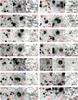 |
Fig. 3 3.6 μm, 24 μm, and 20 cm stamps (30′′ × 30′′ area) for LABOCA COSMOS sources detected by mm-interferometers at ≲2′′ resolution (see Table 3). The bands and sources are indicated in the panels and the names of sources detected with interferometers at S/N > 4.5 are underlined. The thick yellow circle, 2′′ in diameter, indicates the mm-interferometer position. Robust (square) and tentative (diamond) counterparts determined via P-statistic in each particular (3.6 μm, 24 μm, and 20 cm) band are also shown (see text for details; see also Table 6). For each source LABOCA contours in 1σ steps starting at 2σ (with locally determined rms) are overlaid onto the 3.6 μm stamp. |
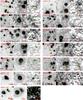 |
Fig. 3 continued. |
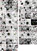 |
Fig. 5 Same as Fig. 3, but for AzTEC/JCMT/SMA COSMOS sources in our 1.1 mm-selected sample (see Tables 1 and 7). The AzTEC/JCMT beam is indicated by the circle in the 3.6 μm stamp. |
5.2.2. Radio counterparts
In our 1.1 mm-selected sample 9/15 (60%) bolometer SMGs have radio sources (drawn from the Joint Deep and Large radio catalogs with rms ~7−12 μJy/beam; Schinnerer et al. 2007, 2010) within the AzTEC beam. This fraction is consistent with that found in (sub)mm-surveys (e.g. Chapman et al. 2005). Only one mm/SMA source (AzTEC-13) in this sample is not associated with a radio source present within the single-dish beam (Younger et al. 2009). Furthermore, AzTEC-5 and AzTEC-8 each have two P-robust radio sources within the AzTEC/JCMT 18′′ beam. In both cases only one radio source is associated with the SMA mm-detection.
Correlating with the Joint VLA-COSMOS Large and Deep catalogs, out of the 36 LABOCA SMGs followed-up with interferometers, 23 (~64%) have radio sources (rms1.4 GHz ≳ 7−12 μJy/beam) within the beam. Of these 36, 26 were detected at mm-wavelengths with interferometers (870 μm-selected sample), and out of these 26, 17 (65%) show radio sources within the LABOCA beam.
Assigning counterparts to each of these LABOCA sources via P-statistic we find that (see Table 6, Figs. 3) in 4 cases (2 with S/N1.3 mm > 4.5)9 the robust/tentative P-counterpart is not coincident with the interferometric-source. Within Poisson uncertainties this is consistent with the results from Younger et al. (2009) for the 1.1 mm-selected sample.
In our 870 μm-selected sample COSLA-161 has a mm-interferometric detection and two P-robust radio counterparts. Multiple P-tentative radio counterparts are found also for COSLA-2, COSLA-5, COSLA-17, and COSLA-73 (three out of these 5 are significant interferometric detections). In all cases, except for COSLA-5, one of the radio sources is associated with the inetrferometric-source.
Combining the above results for our 870 μm-selected sample we thus find 4 cases where the robust/tentative P-counterpart is not associated with the interferometric source, and 4 more ambiguous cases where from the multiple robust/tentative P-counterparts found for the SMG only one is confirmed by the interferometric source. Taking the 26 single-dish SMGs in the 870 μm-selected sample this amounts to a fraction of 15 ± 8% for the first and latter, separately. For the 1.1 mm-selected sample we find one misidentified and two ambiguous SMG counterparts assigned via P-statistic. Taking the 15 single-dish SMGs in the 1.1 mm-selected sample this amounts to 7 ± 7% and 13 ± 7%, respectively.
5.2.3. Radio, 24 μm and IRAC counterparts
In this section we investigate the agreement between robust counterparts determined via P-statistic using radio, 24 μm, and IRAC wavelength regimes, and counterparts identified via intermediate ≲2′′ resolution mm-mapping.
Where both radio and mid-IR data are available, potential counterparts to single-dish detected SMGs are commonly selected by searching for P-statistics robust radio and 24 μm counterparts. Where no such source can be identified, counterparts are searched for among color selected IRAC sources (m3.6 μm − m4.5 μm ≥ 0). In Table 6 and Table 7 we list the resulting P-robust counterparts to the LABOCA and AzTEC samples. A summary of the identifications is given in Table 8.
In the 870 μm-selected sample we find P-robust counterparts for 17 out of the 26 PdBI-identified SMGs – irrespective whether these identification are correct or not. In total we find 18 P-robust counterparts as COSLA-73 and COSLA-161 both have two P-robust counterparts associated. From the 18 statistically identified sources, 12 (66%) are correct identifications based on our PdBI detections. This fraction remains similar if we consider only the single-dish detected SMGs with mm-interferometric detections at S/N > 4.5, i.e. identified without any prior assumptions (i.e. multi-wavelength association): 11/13 (85%) single-dish detected SMGs have P-robust counterparts, in total there are 12 P-robust counterparts (as COSLA-73 is in this sub-sample) and 7 out of these 12 (58%) match our interferometric detections. This amounts to ~50% correct identifications via P-statistic within the samples analyzed (i.e. 7/13 for the least-biased- and 12/26 for the 870 μm-selected sample).
In the 1.1 mm-selected sample we find P-robust counterparts for 8 of 15 (53%) SMGs with SMA detections (Table 7, Fig. 5). Since AzTEC-5 and AzTEC-8 each have two P-robust counterparts, we find 10 P-robust associations in total. Seven of the 10 (70%) are coincident with the mm-interferometric detections. The fraction remains the same if robust and tentative statistical counterparts are considered. Within the Poisson uncertainties this is consistent with the results for the 870 μm-selected sample, i.e. only ~50% of the single-dish detected SMGs have correct counterparts assigned via P-statistic.
5.3. The biases of assigning counterparts to single-dish detected SMGs
Intensive work has been invested into optimizing techniques to determine counterparts to single-dish detected SMGs identified at low (~10–35′′) angular resolution (e.g. Ivison et al. 2002, 2005; Pope et al. 2006; Hainline et al. 2009; Yun et al. 2008, 2012). Deep intermediate-resolution radio observations, which are less time consuming than similar mm-wave observations, but are expected to trace the same physical processes (given the IR-radio correlation; e.g. Carilli & Yun 1999; Sargent et al. 2010) have proven efficient. However, it was realized that radio-counterpart assignment biases samples to low-redshift (e.g. Chapman et al. 2005; Bertoldi et al. 2007). To overcome this, 24 μm- and IRAC color-selected samples have been utilized (e.g. Pope et al. 2006; Hainline et al. 2009; Yun et al. 2008). Generally such methods identify counterparts to ~60% of the parent single-dish SMG sample (e.g. Chapman et al. 2005; Biggs et al. 2011; Yun et al. 2012) and yet the fraction of misidentifications in these samples remains unclear. A further source of bias in such samples is the blending of SMGs within the large single-dish beams. This may potentially be a severe problem as SMGs have been shown to cluster strongly (Blain et al. 2004; Daddi et al. 2009a,b; Capak et al. 2010; Aravena et al. 2010b; Hickox et al. 2012) and reside in close-pairs (as also suggested by simulations; Hayward et al. 2011). Here we provide detailed insight into these issues based on statistical samples.
We have generated two unique (870 μm- and 1.1 mm-selected) SMG samples with counterparts to LABOCA/APEX and AzTEC/JCMT COSMOS SMGs identified via intermediate (≲2′′) resolution mm-mapping (see Sect. 4 and Table 4). Consistent with results from the literature we have found statistical counterparts for ~50–70% of the sources in these samples (see Sect. 5, Tables 6 and 7). Comparing these with the intermediate (≲2′′) resolution mm-detections, we find a ~70% match. If there were no caveats with the intermediate-resolution mm-detections this would imply that statistical counterpart assignment methods utilizing deep radio, 24 μm and IRAC data (such as the one applied here) identify correctly counterparts to ~50% of the parent single-dish samples. Furthermore, it would imply that ≳15%, and possibly up to ~40% of single-dish detected SMGs separate into multiple components, with a median separation of ~5′′, when observed at ≲2′′ angular resolution. The misclassification of statistical assignment is likely intrinsic to the methods applied and also due to the break-up of single-dish SMGs into multiple components. If indeed a large fraction of SMGs are blended within the single dish beams (on scales <10′′), this could affect the slope of the (sub)mm counts inferred from single-dish surveys as the bright end would be overestimated, while the faint end would be underestimated (see Kovaćs et al. 2010, for a more detailed discussion).
We find that radio assignment, relative to near/mid-IR wavelength regimes, is the most efficient tracer of single-dish detected SMG counterparts (see Table 8). Thus, as already demonstrated by Lindner et al. (2011), who find that a 20 cm rms of ~2.7–5 μJy identifies radio counterparts for ~90% of SMGs, future deep radio maps with EVLA, ASKAP, MeerKAT and SKA will provide efficient tracers of SMG counterparts.
Our samples of LABOCA/APEX and AzTEC/JCMT SMGs identified via intermediate (≲2′′) resolution mm-mapping are not complete, but constitute half of the parent SMG samples (see Scott et al. 2008; Navarette et al., in prep.). They are also subject to their own incompletenesses and false detection rates within heterogenous data sets (assembled from SMA, PdBI, and CARMA observations). Thus, although our analysis suggests that roughly half of single-dish detected SMGs are correctly identified via statistical methods, a more robust insight into these issues will have to await further follow-up observations of complete samples of single-dish detected SMGs with higher sensitivities than the ones presented here and with a uniform rms over the full single-dish beam area. One would also preferably want to obtain these data at (at least) two separate frequencies.
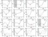 |
Fig. 6 Photometric redshift total χ2 distributions for our SMGs with spectroscopic redshifts. We show results based on various sets of spectral models (see text for details): 2T (dotted lines), 6T (dashed-lines), M (full lines). The spectroscopic redshifts are indicated by vertical dashed lines. The source names and the number of degrees of freedom (dof) in the photometric redshift χ2 minimization are indicated in each panel. The gray-shaded areas in some of the panels indicate the redshift range ignored for the determination of the best-fit photometric redshift. The photometric redshift provided by the best model (M) and its uncertainty was taken as the minimum χ2 value and the 99% confidence interval, respectively, both indicated in each panel by the thick and thin red lines. |
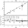 |
Fig. 7 Comparison of spectroscopic and photometric redshifts for 16 starbursts in our COSMOS sample. The photometric redshifts were determined using the Michalowski spectral templates, and the shown errors are ± 3σ errors drawn from the χ2 distributions of the photometric-redshift fits (see Fig. 6 and text for details). The median offset and standard deviation of the Δz/(1 + zspec) distribution are indicated in the bottom panel. Note that for z ≥ 3 we find a slight, 0.04·(1 + z), systematic underestimate of the photometric redshifts. |
6. Distances to submillimeter galaxies
In this section we calibrate photometric redshifts for SMGs based on a sample of 12 SMGs detected via mm-interferometry (and 4 additional high-redshift starburst galaxies) in the COSMOS field with spectroscopic redshifts spanning a broad redshift range of z ~ 0.1−5.3 (see Tables 1 and 2). We optimize the photometric redshift computation, and apply it thereafter to the remainder of our SMG sample.
6.1. Calibration and computation of photometric redshifts for SMGs
Photometric redshifts are computed by fitting optimized spectral template libraries to the spectral energy distribution of a given galaxy, leaving redshift as a free parameter. The redshift is then determined via a χ2 minimization procedure. The quality of the photometric redshifts will depend on the choice of the spectral library. To obtain optimal results for the population of SMGs using Hyper-z, Smolčić et al. (2012) tested three sets of spectral model libraries on a sample of eight SMGs in the COSMOS field with counterparts determined via mm-interferometry and with available spectroscopic redshifts:
-
2T:
Only two – burst and constant star formation history –templates drawn from the Bruzual & Charlot (2003) library (andprovided with Hyper-z).
-
6T:
Six templates provided by the Hyper-z code: burst, four exponentially declining star formation histories (star formation rate ∝ e−t/τ where t is time, and τ = 0.31, 1, 3 and 5 Gyr) and a constant star formation history. This selection of SFH/templates is similar to the approach used by Ilbert et al. (2009) to compute stellar masses with LePhare.
-
M:
Spectral templates developed in GRASIL (Silva et al. 1998; Iglesias-Páramo et al. 2007) and optimized for SMGs by Michalowski et al. (2010).
They find that all three template libraries yield similar results, while the M templates result in the tightest χ2 distributions. Here we repeat their analysis using a larger sample containing 12 SMGs in the COSMOS field with counterparts determined via mm-interferometry and available spectroscopic redshifts. We additionally add to this sample 4 sources (Vd-17871, AK03, AK05, AK07), selected in the same way as AzTEC-1, AzTEC-5, and J1000+0234, i.e. via criteria identifying high-redshift extreme starbursts (Lyman Break Galaxies with weak radio emission; Karim et al., in prep.). The photometric redshifts are computed using the entire available COSMOS photometry (>30 bands) and the Hyper-z code with a Calzetti et al. (2000) extinction law, reddening in the range of AV = 0−5, and allowing redshift to vary from 0 to 7.
The results are shown in Fig. 6, where we present the photometric redshift total χ2 distributions for the 16 sources in our training-set. The overall match between the most probable photometric redshift (corresponding to the minimum χ2 value) and the spectroscopic redshift is good. We emphasize that the sample used for this analysis is rather heterogeneous in respect of redshift range, detections in optical bands, blending, and AGN contribution. For example, Cosbo-3 is a blended source not detected in images at wavelengths shorter than 1 μm (see Smolčić et al. 2012, for details). Constraining its photometric redshift well (as shown in Fig. 6) affirms that our deblending techniques (described in detail in Smolčić et al. 2012), as well as photometric redshift computations work well. Vd-17871 is a weak SMG (with a CO-line detection, and a continuum brightness at 1.2 mm of ~2.5 mJy; Karim et al., in prep.) with substantial AGN contribution identified in the IR (Karim et al., in prep.). Even in this case our photometric redshift agrees well with the spectroscopic redshift. Note also that within our sample with spectroscopic redshifts there are no catastrophic redshift outliers10. For two sources (AzTEC-3 and AK03) there are two equally probable redshift peaks (i.e.  minima). In both cases, however, one of those is consistent with the spectroscopic redshift. In particular, in the case of AzTEC-3 the low redshift peak can be disregarded given that the galaxy is not detected at 1.4 GHz given the depth of the VLA-COSMOS survey.
In conclusion, comparing the redshift probability distributions given the 2T, 6T, and M models, we find that the Michalowski (M) models yield the optimal results (i.e. the tightest redshift probability distributions). Hence, hereafter we will adopt the Michalowski et al. (2010) spectral templates for the photometric redshift estimate for our SMGs. From the redshift probability distribution for a given source we take the most probable redshift (corresponding to that with minimum χ2) as the photometric redshift of the SMG, and derive the 99% confidence interval from its total χ2 distribution. The comparison between photometric and spectroscopic redshifts is quantified in Fig. 7 using the M template library. As already visible from Fig. 6 the photometric and spectroscopic redshifts are in very good agreement. We find a median of −0.02, and a standard deviation of 0.09 in the overall (zphot − zspec)/(1 + zspec) distribution. However, from Fig. 7 it is discernible that the systematic offset is higher for higher redshifts. Fitting z < 3 and z ≥ 3 ranges separately we find a median offset of 0.00, and −0.04, respectively, and a standard deviation of 0.11, and 0.06, respectively. For comparison, a similar median systematic offset (−0.023) has been found by Wardlow et al. (2011) for their full sample of LESS SMGs with statistically assigned counterparts. Yun et al. (2012) find a zero offset for GOODS-South SMGs with statistically assigned counterparts, however their results suggest a slight systematic underestimate of z > 3 photometric redshifts (see their Fig. 2), consistent with the results presented here. This suggests that spectral models used for photometric-redshift estimates could be better optimized for the high-redshift end. This is however beyond the scope of this paper, and here we will correct the (z ≥ 3) photometric redshifts computed for our SMGs for this systematic offset.
Using the same approach as described above we compute photometric redshifts for all SMGs in the COSMOS field with multi-wavelength counterparts determined via mm-interferometry mapping and without spectroscopic redshifts. We present their photometric redshift total χ2 distributions (prior to any systematic correction) in Figs. 8 and 9, and tabulate their photometric redshifts (not corrected for the systematic offset) in Tables 1 and 3.
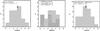 |
Fig. 10 Redshift distribution of our 1.1 mm-selected sample (left panel), 870 μm-selected sample (middle panel), and the two samples combined (with sources present in both samples counted only once; right panel). In the middle panel we also show the redshift distribution of our S/N1.1 mm > 4.5 PdBI-detected LABOCA sample (hatched histogram). Mean redshift values, and corresponding errors obtained using the statistical package ASURV, as well as the number of sources in each sample are indicated in each panel. Mean redshifts for every sample distribution are also indicated by the thick vertical lines. |
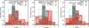 |
Fig. 11 Normalized redshift distributions for SMGs drawn from various studies in the literature, indicated in the panel. |
6.2. AGN considerations
As photometric redshifts are typically computed using libraries for the stellar light only, it may be argued that substantial AGN contribution to the UV-MIR SED for some SMGs may affect our photometric redshift estimate. Note however that only bright Type 1 (broad line) AGN need special treatment for photometric redshift estimates (see Salvato et al. 2010). For low-luminosity (Seyfert, Type 2) AGN, with SEDs dominated by the stellar light of a galaxy (e.g. Kauffmann et al. 2003) usual photometric redshift computations, as the one presented here, are expected to yield satisfactory results.
To address the AGN issue in our SMG sample we have utilized the X-ray data from the Chandra-COSMOS survey (Elvis et al. 2009), which provide the most direct way to identify AGN associated with the SMGs in our 1.1 mm- and 870 μm-selected samples.
Only COSLA-161, for which we find a good agreement between its photometric and spectroscopic redshifts, is found to be associated with X-ray emission (note however that given the X-ray 0.1–10 keV rest-frame luminosity of (6.2 ± 2.7) × 1040 erg s-1 at the source’s low spectroscopic redshift, it is not clear whether the source of X-rays is star-formation or emission from the nucleus; see Appendix for more details). In order to put further constraints on the AGN properties of our SMGs, we derive the average X-ray flux in the 0.5–2 keV band using all COSMOS SMGs with interferometric positions. This is done in such a way that for each SMG we extract the X-ray counts from the 0.5–2 keV band image within a circular aperture of 1.5′′ in radius, and then convert this to an average X-ray flux.
For this stacking analysis we only used the so called best PSF Chandra mosaic (Elvis et al. 2009), that has a continuous coverage of the central 0.5 deg2 of COSMOS at 50 ks depth, in order to be able to use a small extraction region and therefore reduce contamination. The background counts were estimated using the stowed Chandra background data after normalizing the background image to the average background rate in a source-free zone. After background subtraction we find a marginal detection at a 1.5σ level in the stack with F0.5−2keV = (0.9 ± 0.6) × 10-17 erg s-1 cm-2. For SMGs at redshifts z = 2, 3, and 4, and assuming a power-law X-ray spectrum with photon index 1.8 (typical for AGN), the obtained average flux converts to average bolometric X-ray luminosities (rest-frame 0.1–10 keV) of (7.5 ± 5) × 1041, (1.9 ± 1.3) × 1042, and (3.7 ± 2.5) × 1042 erg s-1 (given the marginal detection, these values should be considered as upper limits).
The inferred X-ray luminosities are typical for normal galaxies rather than strong AGN (LX > 1042 erg s-1; e.g. Brusa et al. 2007). This rules out a major AGN contribution within our SMG sample (consistent with previous studies of SMGs; Alexander et al. 2005; Menendez-Delmestre et al. 2009), and thus also a significant influence of AGN on the accuracy of our photometric redshift estimates. Furthermore, as demonstrated by the source Vd-17871 (see previous section and Karim et al., in prep.) buried AGN only obvious in the IR SED do not appear to affect the method. This is consistent with the results from Wardlow et al. (2011) who have found that the accuracy of photometric redshifts is not affected for SMGs showing an IR (8 μm) excess likely due to an AGN component.
7. Redshift distribution of SMGs in the COSMOS field
In this section we present the redshift distributions for our 1.1 mm- and 870 μm-selected samples. To derive the redshift distributions, we take spectroscopic redshifts if available, and otherwise photometric redshifts based on Michalowski et al. (2010) spectral templates, and corrected for the systematic offset as discussed in the previous section (see Table 4).
7.1. Redshift distribution of AzTEC/JCMT SMGs with mm-interferometric positions
Our 1.1 mm-selected sample contains 17 SMGs11 with accurate positions from 890 μm interferometric observations at intermediate resolution (~2′′) with the SMA (Younger et al. 2007, 2009). Spectroscopic redshifts, based on optical (DEIMOS) and/or CO (CARMA/PdBI) spectroscopic observations, are available for 7 out of the 17 AzTEC/JCMT/SMA SMGs (see Table 1). For 7 of the remaining sources we use photometric redshifts, derived as described in Sect. 6. Three sources (AzTEC-11S, AzTEC-13 and AzTEC-14E) cannot be associated with multi-wavelength counterparts in our deep COSMOS images. Thus, for these we use the mm-to-radio flux ratio based redshifts, often utilized for the derivation of distances to SMGs (Carilli & Yun 1999, 2000). Consistent with the faintness at optical, IR, and radio wavelengths the mm-to-radio flux based redshifts suggest z ≳ 3 (see Table 4) for all three sources when the PdBI 1.3 mm fluxes and an Arp 220 template are used (following Aravena et al. 2010a). The redshifts for AzTEC/JCMT COSMOS SMGs are summarized in Table 4.
The redshift distribution for the 17 AzTEC/JCMT SMGs mapped by SMA is shown in the left panel of Fig. 10. Given that for three sources we only have lower redshift limits, we compute the mean redshift using the statistical package ASURV which relies on survival analysis, and takes upper/lower limits properly into account (assuming that sources with limiting values follow the same distribution as the ones well constrained). We infer a mean redshift of 3.06 ± 0.37 for the AzTEC/JCMT/SMA sources. We note that treating the source AzTEC-11 as a single source yields a mean redshift of 3.00 ± 0.38.
7.2. Redshift distribution of LABOCA-COSMOS SMGs with mm-interferometric positions
Unlike the 1.1 mm-selected sample, the 870 μm-selected one is not strictly limited in flux or signal-to-noise. This is because a fraction of S/N870 μm ≳ 3.8 LABOCA-COSMOS SMGs have not been detected by our PdBI observations at 1.3 mm. The least biased sample that can be constructed from these detections is a sample of the LABOCA-COSMOS sources detected with interferometers at mm-wavelengths, but without prior assumptions, such as e.g. multi-wavelength counterpart associations (as described in Sect. 3, we required that our S/N1.3 mm ≤ 4.5 PdBI sources had to be confirmed by independent multi-wavelength detections). This yields 16 sources (9 PdBI detected with S/N > 4.5, and 7 detected with SMA or CARMA12) in our least-biased 870 μm-selected sample, listed in Table 4. It is hard to assess the completeness of this sample. However, if our detection rate of the LABOCA sources can be considered random i.e. devoid of any redshift-biases, and the properties of the non-detected LABOCA sources are similar to those of the detected ones, then one can assume that this subsample reflects the distribution of the parent LABOCA SMG sample within the same flux limits. Furthermore, note that the 9 LABOCA/PdBI sources detected with S/N1.3 mm > 4.5 within our least-biased 870 μm-selected sample can be regarded as a 1.3 mm flux-limited sample (F1.3 mm ≳ 2.1 mJy; given that we reached an rms of ~0.46 mJy in our PdBI maps). Hence, if the redshift distribution of the least-biased 870 μm-selected sample is consistent with that of the PdBI sub-sample, we can assume that this reflects the distribution of SMGs with F1.3 mm ≳ 2.1 mJy.
Five out of the 16 SMGs in our least-biased 870 μm-selected sample13 have spectroscopic redshifts. For another eight we use photometric redshifts as derived in Sect. 6, and for 3 others we use the mm-to-radio flux based redshifts. Their redshift distribution, shown in the middle panel of Fig. 10, is similar to that of the PdBI subsample. Using the ASURV statistical package we infer a mean redshift of 2.59 ± 0.36, and 2.29 ± 0.48 for the least-biased 870 μm-selected sample, and the PdBI S/N1.3 mm > 4.5 subsample, respectively.
Given the faintness of the counterpart of COSLA-17-S its photometric redshift ( ) is rather poorly constrained, and discrepant compared to the mm-to-radio based one (≳4). Thus it is possible that this source is at high redshift and further mm-observations of COSLA-17-N are required to affirm the reality of this source (see Appendix A for details). Nonetheless, excluding COSLA-17 N and S from the sample, we obtain consistent mean redshifts for the least-biased 870 μm-selected sample (2.65 ± 0.38) and the PdBI S/N > 4.5 subsample within (2.34 ± 0.55).
We show the redshift distribution of the joint 1.1 mm-selected sample and least-biased 870 μm-selected sample in the right panel of Fig. 10. A mean redshift of 2.80 ± 0.2814 is found. A comparison with results from literature is given in Fig. 11 and discussed in detail in Sect. 8.
8. Discussion
8.1. The redshift distribution of SMGs
In Fig. 11 we compare the (normalized) redshift distribution of the AzTEC/JCMT/SMA (left panel) and LABOCA/ interferometric (middle panel) COSMOS samples, and their joint distribution (right panel), with redshift distributions of SMGs derived for other surveys (Chapman et al. 2005; Banerji et al. 2011; Wardlow et al. 2011; Yun et al. 2012). The redshift distribution derived by Chapman et al. (2005) is based on a sample of 76 SMGs drawn from various SCUBA 850 μm surveys with counterparts identified via radio sources present within the SCUBA beam, and observed with Keck I to obtain optical spectroscopic redshifts (see their Table 2). To account for the redshift desert at z = 1.2−1.7 in the Chapman et al. sample we supplement it with 19 SMGs with DEIMOS spectra drawn from Banerji et al. (2011, see their Table 2). We combine these two data sets normalizing each by the observed area (556 arcmin2 for the Banerji et al., and 721 arcmin2 for the Chapman et al. samples; Chapman, priv. comm.).
The distribution published by Wardlow et al. (2011) is based on 74 SMGs drawn from the LESS survey at 870 μm that could be assigned robust counterparts based on the P-statistic (using radio, 24 μm and IRAC data; Biggs et al. 2011). Wardlow et al. derived photometric redshifts for these galaxies (see their Table 2) accurate to σΔz/(1 + z) = 0.037. Using the P-statistic to associate counterparts to SMGs (although using a slightly modified method to that utilized by Biggs et al. 2011) Yun et al. (2012) identified 44 (robust and tentative) counterparts to SMGs detected with AzTEC at 1.1 mm in the GOODS-S field. For 16 sources in this sample a spectroscopic redshift is used, for 21 a photometric redshift was inferred by Yun et al., and for 7 only a mm-to-radio based redshift could be derived (see their Table 3).
From Fig. 11 it is immediately obvious that the redshift distribution of the COSMOS SMGs is much broader compared to that derived from previous surveys, in which the SMG counterparts were identified statistically within the large bolometer beam. In particular, significant high-redshift (z ≳ 4) and low-redshift (z < 2) ends are present. In the 870 μm-selected sample we find five15 out of 16 SMGs (i.e. ~30%) at z < 1.5. While the redshifts of two of these are spectroscopically confirmed, the photometric redshifts for the other three show possible secondary (higher) redshift solutions, which are more consistent with their mm-to-radio flux based redshifts. In our 1.1 mm-selected sample we find four16 out of 17 (23.5%) SMGs at z < 1.5. The redshifts for three of these are spectroscopically confirmed. Thus, in total we find roughly 20–30% of SMGs at z < 1.5 (see left and middle panels in Fig. 11). Such low redshift SMGs, present in the combined Chapman et al. (2005) and Banerji et al. (2011) sample but interestingly missed in the 1.1 mm AzTEC-GOODS-S and 870 μm-LESS samples, are expected in models of the evolution of infrared galaxies (see e.g. Fig. 7 in Béthermin et al. 2011), and they could be explained by cold dust temperatures in these sources (e.g. Greve et al. 2006; Banerji et al. 2011). A more detailed analysis of the physical properties of these SMGs will be presented in an upcoming publication.
We find significantly more SMGs at the high-redshift end (z ≳ 4) in both our 1.1 mm- and least-biased-870 μm-selected samples, compared to the other surveys. As discussed in detail by Chapman et al. (2005) and Wardlow et al. (2011) this is likely due to the low-redshift bias of statistical counterpart assignment methods. Using statistical means to overcome this bias Wardlow et al. (2011) estimate that ~30% (and at most ~45%) of all SMGs in their sample are at redshifts z ≳ 3. Our combined AzTEC/JCMT/SMA and LABOCA/interferometric COSMOS data yield that ~50% of the COSMOS SMGs with interferometrically identified counterparts are at z ≳ 3. Exploring these two samples separately, we find that ~50% (i.e. 9/17) of the AzTEC/JCMT/SMA SMGs, and ~40% (i.e. 6/16) of the LABOCA/interferometric SMGs have z ≳ 3.
It is possible that the discrepancies between the z ≳ 3 SMG fractions in these different samples are due to their different average flux densities. Namely, past studies have suggested the existence of a correlation between SMG brightness and redshift, in such a way that the brightest SMGs lie at the highest redshift (e.g. Ivison et al. 2002; Pope et al. 2005; Biggs et al. 2011). The LESS survey source flux limit is F870 μm > 4.4 mJy (Biggs et al. 2011). Assuming a power-law of 3 this translates into a limit of 2.2 mJy at 1.1 mm, and 1.3 mJy at 1.3 mm. The AzTEC/JCMT/SMA COSMOS source flux limit is F1.1 mm > 4.2 mJy, thus about 2 times higher, and the LABOCA/PdBI limit is ≳2.1 mJy, thus a factor of 1.6 higher compared to the LESS sample. Indeed, we find higher mean redshifts ( = 3.1 ± 0.4 for the 1.1 mm-selected sample, and = 2.6 ± 0.4 for the 870 μm-selected sample) and thus also a higher fraction of high-redshift sources compared to the results based on the LESS survey ( ). This is consistent with the suggestions from past studies that on average brighter SMGs are at higher redshifts. On the other hand, it has also been suggested that mm-selected samples lie on average at higher redshifts, compared to sub-mm-selected samples (e.g. Yun et al. 2012). Although our results are also consistent with this hypothesis, a more conclusive answer, disentangling these degeneracies, will have to await for deeper mm- and sub-mm selected samples with interferometric counterparts and accurately determined redshifts.
8.2. High redshift SMGs
In our 1.1 mm-, and 870 μm-selected samples we find 9 (3 of which have radio counterparts) and 8 (4 of which have radio counterparts) z ≳ 3 SMGs. We find 5–817 SMGs at z ≳ 4 in our 1.1 mm-selected sample, and and 3–418 SMGs at z ≳ 4 in our 870 μm-selected sample. This corresponds to ~30–50% of the 1.1 mm-selected sample, and ~20% of the 870 μm-selected sample. As our 870 μm-selected sample, is not complete, we can infer only a lower limit for the z ≳ 4 SMG surface density of ≥ 3/0.7 ≈ 4 deg-2. The 1.1 mm-selected sample is however nearly complete at the given 1.1 mm flux limit of F1.1 mm > 4.2 mJy, and drawn from a uniform area of 0.15Λ°. Four SMGs (AzTEC-1, 3, 4, and 5) in the 1.1 mm-selected sample are found to be at z ≳ 4 (three of those have spectroscopic redshifts; see Table 4). J1000+0234, with a 1.1 mm flux of 4.8 ± 1.5 mJy (i.e. ~3σ and thus not included in our 1.1 mm-selected sample), is also spectroscopically confirmed to be at z > 4 (Capak et al. 2008, Schinnerer et al. 2008). Furthermore, only lower redshift limits are available for AzTEC-11S, 13 and 14E. Thus, these three SMGs may possibly also lie at z ≳ 4. Hence, these 5–8 z ≳ 4 SMGs with F1.1 mm > 4.2 mJy in the 0.15Λ° field yield a surface density in the range of ~34 ± 14 deg-1 to ~54 ± 18 deg-1 (Poisson errors). Both values are substantially higher than what is expected in cosmological models (Baugh et al. 2005; Swinbank et al. 2008; see also Coppin et al. 2009, 2010), even if the AzTEC/JCMT-COSMOS field were affected by cosmic variance of to a factor of 3 overdensity, as suggested by Austermann et al. (2009).
Based on the galaxy formation model of Baugh et al. (2005; top-heavy IMF; Λ cold dark matter cosmology) a surface density of ~7 deg-1 for z > 4 SMGs with 850 μm fluxes brighter than 5 mJy is expected (see also Swinbank et al. 2008; Coppin et al. 2009). As the AzTEC/JCMT/SMA 4.2 mJy flux limit at 1.1 mm translates to about a factor of two higher flux (i.e. 9.6 mJy) at 850 μJy, the models would predict an even lower surface density at this flux threshold.
In the GOODS-N field to date four z > 4 SMGs were found (Daddi et al. 2009a,b; Carilli et al. 2011). Given the 10 × 16.5 arcmin2 area (but with a highly non uniform rms in the SCUBA map with average 1σ = 3.4 mJy; Pope et al. 2005) this implies a surface density of ≳87 deg-2, an order of magnitude higher than predicted by the models. The GOODS-N z > 4 SMGs are however associated with a protocluster at z ~ 4.05 which increases the surface density value. The COSMOS z > 4 SMGs were selected from a larger field, and although an overall overdensity of bright SMGs was found in the AzTEC/JCMT-COSMOS field (Austermann et al. 2009), the z > 4 SMGs do not seem to be associated with each other (Capak et al. 2009, 2010; Schinnerer et al. 2009; Riechers et al. 2010; Smolčić et al. 2011). We still find significantly more z > 4 SMGs than current models predict. If the AzTEC/JCMT COSMOS SMGs are representative of the overall SMG population (F1.1 mm > 4.2 mJy), then our results imply that current semi-analytic models underpredict the number of high-redshift starbursts.
9. Summary
We presented PdBI continuum observations at 1.3 mm with ~1.5′′ angular resolution and an rms noise level of ~0.46 mJy/beam towards 28 SMGs selected from the (single-dish) LABOCA-COSMOS survey of 27′′ angular resolution. Nine SMGs remain undetected, while the remainder yields 9 highly significant (S/N > 4.5) and 17 tentative (3 < S/N ≤ 4.5 with multi-wavelength source association required) detections. Combining these with other single-dish identified SMGs detected via intermediate (≲2′′) angular resolution mm-mapping in the COSMOS field we present the largest sample of this kind to-date, containing 50 sources. Based on 16 interferometrically confirmed SMGs with spectroscopic redshifts, we show that photometric redshifts derived from optical to MIR photometry are as accurate for SMGs as for other galaxy populations. We derived photometric redshifts for those SMGs in our sample which lack spectroscopic redshifts.
We distinguish two statistical samples within the total sample of 50 COSMOS SMGs detected at ≲2′′ angular resolution at mm-wavelengths: i) a 1.1 mm-selected sample, forming a significance- (S/N1.1 mm > 4.5) and flux-limited (F1.1 mm > 4.2 mJy) sample containing 17 SMGs with interferometric positions drawn from the AzTEC/JCMT 0.15Λ° COSMOS survey, and ii) a 870 μm-selected sample, containing 27 single-dish SMGs drawn from the LABOCA 0.7Λ° COSMOS survey and detected with various (CARMA, SMA, PdBI) mm-interferometers at intermediate angular resolution.
Within our samples we find that ≳15%, and up to ~40% of single-dish identified SMGs tend to separate into multiple components when observed at intermediate angular resolution.
The common P-statistics counterpart identification correctly associates counterparts to ~50% of the parent single-dish SMG samples analyzed here.
We derive the redshift distribution of the SMGs with secure counterparts identified via intermediate ≲2′′ resolution mm-observations, and compare this distribution to previous estimates that were based on statistically identified counterparts. We find a broader redshift distribution with a higher abundance of low- and high-redshift SMGs. The mean redshift is higher than in previous estimates. This may add evidence to previous claims that brighter and/or mm-selected SMGs are located at higher redshifts.
We derive a surface density of z ≳ 4 SMGs (F1.1 mm ≳ 4.2 mJy) of ~34–54 deg-1, which is significantly higher than what has been predicted by current galaxy formation models.
Online material
Appendix A: Notes on individual LABOCA-COSMOS targets observed with the PdBI
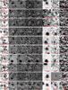 |
Fig. A.1 Optical to radio stamps for the LABOCA-COSMOS SMGs detected by PdBI. Names of sources with S/N > 4.5 in PdBI maps are underlined. |
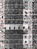 |
Fig. A.1 continued. |
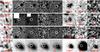 |
Fig. A.1 continued. |
 |
Fig. A.2 Cleaned PdBI maps (color scale), 30′′ on the side, with ± 2σ,3σ,... contours overlaid. Detections (identified in the dirty maps, see text for details) are marked by crosses. |
Here we present detailed notes on individual LABOCA-COSMOS (i.e. COSLA) SMGs observed with PdBI at 1.3 mm and ~1.5′′ resolution. We use a spectral index of 3, i.e. assuming Sν ∝ ν2 + β, where Sν is the flux density at frequency ν and β = 1 the dust emissivity index, to convert fluxes from/to various (sub-)mm wavelengths (if not stated otherwise).
COSLA-5
COSLA-5 is a S/N = 4.1 detection located at α = 10 00 59.521, δ = + 02 17 02.57. The PdBI-source is found at a separation of 3.4′′ from the LABOCA source center. The 1.3 mm flux density of the source is 2.04 ± 0.49 mJy. Scaling this to the MAMBO (1.2 mm) and LABOCA (870 μm) wavelengths we find 2.6 ± 0.6 and 6.9 ± 1.7 mJy, respectively. This is slightly lower than the extracted (and deboosted) MAMBO and LABOCA fluxes (4.78 ± 1, and 12.5 ± 2.6 mJy) and may indicate the presence of another mm-source, not detected in our PdBI map. Based on the rms reached in the PdBI observations, we can put a 3σ upper limit to this potential second source of 1.4 mJy.
The PdBI peak is 1.3′′ away from a source that is independently detected in the optical (i + = 22.5), UltraVista, and IRAC bands. The photometric redshift of this source is well constrained,  . Interestingly, at a separation of 1.1′′ towards the SW of the PdBI detection we find a faint source present only in the Ks band images, but not included in the catalogs (it is present in both the WIRCam and UltraVista images).
The mm-source is not associated with a radio detection suggesting a mm-to-radio flux based redshift for COSLA-5 of zmm/radio ≳ 3.8. Here we take the optical/IRAC/UltraVista source as the counterpart noting that given the ~4σ significance of the PdBI peak, and a separation of ≳1′′ from multi-wavelength sources, further follow-up is required to confirm this source and its redshift.
COSLA-6
Two significant (S/N > 4.5) sources are detected within the COSLA-6 PdBI map.
COSLA-6-N (S/N = 5.4, α = 10 01 23.64, δ = + 02 26 08.42) has a 230 GHz (1.3 mm) flux density of 2.7 ± 0.5 mJy. No IRAC/UltraVista source is found nearby. The closest source is a faint optical (no UltraVista/IRAC/radio) source 2.0′′ away. Given the high significance of the mm-detection the mm-positional accuracy is ~0.3′′. Thus, it seems unlikely that this optical source is the counterpart of the mm-detection. COSLA-6-N is however coincident with a 2.1σ peak in the radio map (F1.4 GHz = 19.5 ± 9.4 μJy). Based on this, we infer a mm-to-radio flux based redshift of 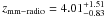 .
.
COSLA-6-S (S/N = 4.75, α = 10 01 23.57, δ = + 02 26 03.62) has a 1.3 mm flux density of 3.1 ± 0.6 mJy. It might be associated with a source detected in the optical (separation = 0.5′′; i + = 26.15), but not in near- or mid-IR. It is coincident with a 3.3σ peak in the radio map (F1.4 GHz = 33.3 ± 10.1 μJy). Based on the multi-wavelength photometry, we infer a photometric redshift of  for this source. A second potential redshift solution (although not as likely as the first one) exists at z ~ 4, and it is supported by the mm-to-radio flux based redshift,
 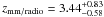 .
.
The combined 1.3 mm fluxes of COSLA-6-N and COSLA-6-S, scaled using a spectral index of 3, yield an expected flux density of 19.4 ± 2.7 mJy at 870 μm. This is in very good agreement with the deboosted LABOCA 870 μm flux of 16.0 ± 3.4.
COSLA-8
COSLA-8 is detected at S/N = 4.2, and located at α = 10 00 25.55, δ = +02 15 08.44. Its 1.3 mm flux density is F1.3 mm = 2.65 ± 0.62 mJy. Using a spectral index of 3 this extrapolates to an 870 μm flux density of 8.9 ± 2.1 mJy, in good agreement with the LABOCA deboosted flux of 6.9 ± 1.6 mJy. The source is located in a crowded region. A radio, IRAC, UltraVista detection is present at a separation of ~3′′, however the closest source to the mm-source (separation = 1.0′′) is detected only in the optical (i + = 27.4). A 3.3σ peak is found at the mm-position in the radio map (F1.4 GHz = 26.2 ± 8.0 μJy). The most probable photometric redshift for this source is  , however with a rather flat χ2 distribution as reflected in the uncertainties.
COSLA-9
We identify two 3.2σ peaks at α = 10 00 13.83, δ = + 01 56 38.64 (COSLA-9-S; 5.8′′ away from the LABOCA source center), and α = 10 00 13.75, δ = + 01 56 41.54 (COSLA-9-N; 7′′ away from the LABOCA source center). COSLA-9-S can be matched to an optical/IRAC/UltraVista source (i + = 24.8, separation = 0.8′′), while the closest source to COSLA-9-N is detected only in the optical (i + = 26.1; separation = 0.4′′) however it is only 1.3′′ away from an optical/UltraVista/IRAC source.
The primary beam corrected 1.3 mm flux densities of COSLA-9-N and COSLA-9-S are 1.69 ± 0.47 mJy, and 1.87 ± 0.58 mJy, respectively. Added together, and scaled to the LABOCA (13.2 ± 2.1 mJy) and AzTEC (6.3 ± 1.0 mJy) frequencies yields a good match to the deboosted LABOCA (14.4 ± 3.3 mJy) and AzTEC (8.7 ± 1.1 mJy) fluxes. Given the low significance of the sources, further follow-up is required to confirm their reality.
COSLA-10
No significant source is present in the 1.3 mm map. The statistical counterpart association (see Sect. 5.2.1 and Fig. 4 for details) suggests three separate potential (tentative) counterparts to this LABOCA source. The sum of the extracted 1.3 mm fluxes (taken as maximum flux within a circular area of 1′′ in radius centered at the statistical counterpart), corrected for the primary beam response, is 2.43 mJy. This yields a flux of 8.1 mJy when scaled to 870 μm, in very good agreement with the LABOCA flux of 7.3 ± 1.7 mJy (see Fig. 2). This suggests that the LABOCA source may be fainter at 1.3 mm than can be detected given our PdBI sensitivity and that it possibly breaks up into multiple components when observed at 1.5′′ resolution.
COSLA-11
The brightest peaks in the PdBI map are at 3.5σ (COSLA-11-N) and 3σ (COSLA-11-S).
COSLA-11-N is located at α = 10 01 14.260, δ = 01 48 18.86, and it can be associated with a faint optical detection 0.64′′ away (i + = 27.75). Its 1.3 mm flux density is F1.3 mm = 2.15 ± 0.62 mJy, and the source is not detected in the radio map. Based on the multi-wavelength photometry of the counterpart of COSLA-11-N, we find a photometric redshift of  . The mm-to-radio based redshift however suggests zmm/radio ≳ 3.6.
COSLA-11-S (α = 10 01 14.200, δ = + 01 48 10.31) is only 2.6′′ away from the center of the LABOCA source, and it coincides (separation = 0.5′′) with independent optical and UltraVista H-band, and UltraVista J-band detections. Although fairly low S/N, the UltraVista detection increases the probability that it is a real source. Its 1.3 mm flux density is F1.3 mm = 1.43 ± 0.48 mJy. Our photometric redshift estimate yields two, almost equally probable, redshifts at z ~ 0.2 and z ~ 3. Given that the SMG is not detected in the radio map, the higher redshift solution, also consistent with the mm-to-radio flux ratio based redshift (zmm/radio ≳ 3), is more likely. We thus adopt the higher redshift solution for this source yielding  (where the errors reflect the 99% confidence interval derived using only z > 1.5 χ2 values).
The combined flux densities of the two detections, scaled to 870 μm, yield a flux density of 12.0 ± 2.6 mJy at this wavelength. This is in good agreement with the LABOCA 870 μm flux density of 19.4 ± 4.5 mJy, and thus further affirms the reality of the sources.
COSLA-12
No significant source is present in the 1.3 mm map. The statistical counterpart association (see Sect. 5.2.1 and Fig. 4 for details) suggests two separate potential (one robust and one tentative) counterparts to this LABOCA source. The sum of the extracted 1.3 mm fluxes (taken as the maximum flux within a circular area of 1′′ in radius centered at the statistical counterpart), corrected for the primary beam response, is 2.68 mJy. Scaled to 870 μm this implies a flux of 8.9 mJy which is lower than the LABOCA flux of 18.3 ± 4.2 mJy (see Fig. 2). This suggests that the LABOCA source may be fainter at 1.3 mm than can be detected given our PdBI sensitivity and/or it breaks up into multiple components when observed at 1.5′′ resolution.
COSLA-13
COSLA-13 is detected at S/N = 3.9 (α = 10 00 31.840, δ = +02 12 42.81). Its 1.3 mm flux density is F1.3 mm = 1.37 ± 0.61 mJy. This SMG is detected within the LABOCA (870 μm), AzTEC (1.1 mm), and MAMBO (1.2 mm) surveys. Scaling the PdBI 1.3 mm flux to 870 μm, 1.1 mm, 1.2 mm (using a slope of 4.6 which corresponds to the mean slope between the AzTEC/LABOCA and AzTEC/MAMBO detected fluxes) we find flux densities of 8.8 ± 3.9 mJy (870 μm), 2.9 ± 1.3 mJy (1.1 mm), and 2.0 ± 0.9 mJy (1.2 mm). These are consistent with the AzTEC/LABOCA fluxes, and slightly lower than the MAMBO flux (note that we find consistent results when using a slope with a spectral index of 3).
The PdBI mm-source is coincident with an optical/UltraVista/IRAC/radio source (separation = 0.55′′) with an optical spectrum at redshift zspec = 2.175.
COSLA-14
No significant source is present in the 1.3 mm map. The statistical counterpart association (see Sect. 5.2.1 and Fig. 4 for details) suggests one robust statistical counterpart to this LABOCA source. The extracted 1.3 mm flux (taken as maximum flux within a circular area of 1′′ in radius centered at the statistical counterpart), corrected for the primary beam response, is 1.64 mJy. The scaled 870 μm flux of 5.5 mJy is fairly consistent with the LABOCA flux of 9.0 ± 2.1 mJy when scaled to 870 μm (see Fig. 2). This suggests that the LABOCA source may be fainter at 1.3 mm than can be detected given our PdBI sensitivity.
COSLA-16
A significant extended source is found ~3.5′′ away from the LABOCA source center. It is best fit by a double-Gaussian (using the AIPS task jmfit and fixing the width of the Gaussians), yielding two sources located at α = 10 00 51.5854, δ = + 02 33 33.5648 (COSLA-16-N) and α = 10 00 51.5541, δ = + 02 33 32.0948 (COSLA-16-S). The 2-Gaussian fit yields 1.3 mm flux densities of F1.3 mm = 1.39 ± 0.32 mJy (COSLA-16-N) and F1.3 mm = 1.19 ± 0.33 mJy (COSLA-16-S).
COSLA-16-N can be associated with an optical/UltraVista/ IRAC/radio source (separation = 0.79′′). COSLA-16-S is not associated with a separate source in the multi-wavelength catalogs. The radio emission associated with the position of COSLA-16-N is significant (F1.4 GHz = 95.6 ± 10.1 μJy), while a 3.3σ peak, that seems to be the extension of the significant radio source, is associated with COSLA-16-S (F1.4 GHz = 33.3 ± 10.1 μJy). The multi-wavelength photometry of COSLA-16-N implies a photometric redshift of  . The mm-to-radio based redshift inferred for COSLA-16-S is
 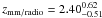 , suggesting it is associated with COSLA-16-N.
Photometry table for our LABOCA SMGs with PdBI detections.
A third 3.9σ peak (COSLA-16-E) with 1.3 mm flux density of F1.3 mm = 2.26 ± 0.58 mJy is found 6′′ east of the LABOCA source center and it is coincident with a faint optical source (separation = 0.41′′, i + = 29.20). Our photometric redshift computation yields s redshift of  , however (as also reflected in the error) the χ2 distribution is fairly flat below z ≲ 4 thus making all redshifts below z ~ 4 almost equally probable. The mm-to-radio flux based redsfhit suggests zmm/radio ≥ 3.7.
The combined 1.3 mm flux density of the 3 identified sources, scaled to 870 μm yields 16.3 ± 2.5 mJy, in very good agreement with the deboosted LABOCA flux (14.0 ± 3.6 mJy).
COSLA-17
Two significant S/N > 4.5 detections are found within the PdBI map.
COSLA-17-S is detected at high significance (S/N = 5.3; α = 10 01 36.772, δ = + 02 11 04.87). Its 1.3 mm flux density is F1.3 mm = 3.0 ± 0.6 mJy, and it can be associated with a faint source 0.23′′ away with mNB816 = 26.2. No IR or radio source is associated with this detection. We find a photometric redshift for this source of  , while the mm-to-radio based redshift suggests zmm/radio ≳ 4.
COSLA-17-N is found at S/N = 4.6 (α = 10 01 36.811, δ = + 02 11 09.66) with a 1.3 mm flux density of F1.3 mm = 3.55 ± 0.677 mJy. It is perfectly coincident with an optical/UltraVista/IRAC/radio source (separation = 0.09′′), however it is within the sidelobe region of the brighter COSLA-17-S source. Hence further follow-up with more complete uv-coverage is required to affirm this source. We find a photometric redshift of  , consistent with the mm-to-radio based redshift of
 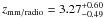 .
.
This SMG is detected by both LABOCA and AzTEC/ASTE surveys, and the flux ratio using these two surveys suggests a spectral index of 2.08. Using this value to scale the combined 1.3 mm PdBI fluxes to 870 μm (1.1 mm) we find a flux density of 15.2 ± 2.2 mJy (9.2 ± 1.4 mJy), consistent with the deboosted LABOCA (AzTEC/ASTE) flux of 12.5 ± 3.2 mJy ( mJy).
mJy).
COSLA-18
COSLA-18 is detected at S/N = 4.5 (α = 10 00 43.19, δ = + 02 05 19.17). Its 1.3 mm flux density is F1.3 mm = 2.15 ± 0.48 mJy. Scaled to 870 μm (1.1 mm) this yields a flux density of 7.2 ± 1.6 mJy (3.5 ± 0.8 mJy), consistent with the deboosted LABOCA (AzTEC/ASTE) fluxes of 10.0 ± 2.6 mJy ( mJy). The source is coincident with an optical/UltraVista/IRAC/radio source (separation = 0.67′′; i + = 28.96). Our photometric redshift computation yields 2 almost equally probable photometric redshifts at z ~ 3 and z ~ 5. The significant radio detection (F1.4 GHz = 60.1 ± 8.9 μJy) would argue in favor of the lower redshift solution, consistent with the mm-to-radio flux based redshift of
 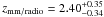 . Thus, here we adopt the low-redshift solution for this source, yielding
  , noting that a second solution of
  is possible.
COSLA-19
Cosla-19 is detected at S/N = 4.1 with a 1.3 mm flux density of 3.17 ± 0.76 mJy. Scaling this flux to 1.2 mm, 1.1 mm, and 870 μJy yields fluxes of 4.1 ± 1.0 mJy, 5.1 ± 1.2 mJy, 10.7 ± 2.6 mJy, respectively, consistent with the deduced MAMBO, AzTEC, and LABOCA fluxes of 5.55 ± 0.9 mJy,  mJy, and 7.4 ± 1.8 mJy, respectively. The closest multi-wavelength source to Cosla-19 is an optical/UltraVista source 2.0′′ away (i + = 25.66). Such a separation makes it unlikely that this source is the counterpart of the mm-detection although given the mm-resolution and significance a ~0.8′′ positional uncertainty is expected. A 2σ = 16.1 μJy radio peak is associated with the PdBI mm peak yielding a mm-to-radio-flux ratio based redshift for Cosla-19 of
 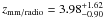 .
.
COSLA-23
Within the COSLA-23 LABOCA beam two significant (S/N > 5) sources are found in the PdBI 1.3 mm map. COSLA-23-N is detected at S/N = 7.3 at α = 10 00 10.161, δ = + 02 13 34.95. It is coincident with an optical/UltraVista/IRAC/radio source (separation = 0.44′′; i + = 26.3). COSLA-23-S is detected at S/N = 6.2 at α = 10 00 10.070, δ = + 02 13 26.87. It can be matched to an optical/IRAC source (separation = 0.87′′, i + = 28.49), but it is not detected in the radio map. Based on the multi-wavelength photometry of the counterparts we find photometric redshifts of  (COSLA-23-N) and
  (COSLA-23-S).
The 1.3 mm flux densities for COSLA-23-N and COSLA-23-S are 3.42 ± 0.47 mJy, and 3.70 ± 0.60 mJy, respectively. Only COSLA-23-N is within the MAMBO 11′′ beam, and the scaled 1.3 mm flux (4.4 ± 0.6 mJy) agrees well with the COSBO-2 flux (5.77 ± 0.9 mJy).
COSLA-25
No significant source is present in the 1.3 mm map. No statistical counterpart could be associated with this SMG. Therefore, it remains unclear whether the LABOCA source is spurious, breaks up into multiple components at 1.5′′ angular resolution, or simply is below the PdBI detection limit.
COSLA-30
No significant source is present in the 1.3 mm map. No statistical counterpart could be associated with this SMG. Therefore, it remains unclear whether the LABOCA source is spurious, breaks up into multiple components at 1.5′′ angular resolution, or simply is below the PdBI detection limit.
COSLA-33
The most prominent feature in the PdBI map within the LABOCA beam is a 3.1σ peak 6.0′′ away from the LABOCA source center that can be associated with an optical/ UltraVista/IRAC source (i + = 25.2, separation = 0.95′′). Its 1.3 mm flux density is 1.78 ± 0.58 mJy which scales to 6.02 ± 1.95 mJy at 870 μm, in good agreement with the deboosted LABOCA flux (6.8 ± 1.1 mJy). Given the low significance of the 1.3 mm source further follow-up is required to affirm its reality.
COSLA-35
COSLA-35 is detected at a signal-to-noise of S/N = 4.2 (α = 10 00 23.65, δ = + 02 21 55.22). Its 1.3 mm flux density is F1.3 mm = 2.15 ± 0.51 mJy. This flux scaled to 870 μm (1.1 mm) yields a flux density of 7.3 ± 1.7 mJy (3.5 ± 0.8 mJy), consistent with the observed LABOCA (AzTEC/ASTE) fluxes of 8.2 ± 1.1 mJy ( mJy). The mm-detection is coincident with an optical/UltraVista/IRAC/radio source (separation = 0.55′′; i + = 27.24). We find a photometric redshift of
  .
.
COSLA-38
COSLA-38 is detected at S/N = 4.4 at α = 10 00 12.59, δ = + 02 14 44.31, 14.8′′ away from the LABOCA source position (thus essentially outside the LABOCA beam; FWHM = 27′′). It is however only 0.67′′ away from the MAMBO source Cosbo-19, and coincident with a radio/UltraVista/IRAC/optical source (separation = 0.23′′, i + = 24.08). We infer a 1.3 mm flux density of F1.3 mm = 8.19 ± 1.85 mJy, which should however be treated with caution as the correction for the primary beam response at that distance from the PdBI phase center applied to the flux is about a factor of 4. We find a photometric redshift of  for this SMG.
COSLA-40
COSLA-40 is detected at S/N = 3.4 (α = 09 59 25.91, δ = + 02 19 56.40), 11.3′′ away from the LABOCA source center. Its 1.3 mm flux density is F1.3 mm = 3.41 ± 1.02 mJy. Scaling this flux to 870 μm yields a flux density of 11.5 ± 3.4 mJy, in very good agreement with the deboosted LABOCA flux (F870 μm = 11.1 ± 3.4 mJy). The source is coincident with an optical source (separation = 0.51′′; i + = 25.52), but not detected in the radio. Given the expected flux density, and the coincidence of the source with an optical detection we assume this source to be real. We find a photometric redshift of  , but we note that χ2 dips are also found at lower and higher redshift values, and that the mm-to-radio flux based redshift suggests zmm/radio ≳ 4.5.
COSLA-47
COSLA-47 is detected at α = 10 00 33.350, δ = + 02 26 01.66 and S/N = 5.3, 6.4′′ away from the LABOCA source center. Its 1.3 mm flux density is 3.11 ± 0.59 mJy, and consistent with the LABOCA/AzTEC fluxes, when scaled to these frequencies. The PdBI source is coincident (separation = 0.48′′) with a source independently detected at optical, IR, and radio wavelengths. We find a well constrained photometric redshift of  .
.
Within the LABOCA beam several more S/N > 4 peaks can be associated with optical/UltraVista/IRAC sources. They are however within sidelobe contaminated regions. This LABOCA SMG may be a blend of several sources, but further follow-up is required to confirm this.
COSLA-48
No significant source is present in the 1.3 mm map. The statistical counterpart association (see Sect. 5.2.1 and Fig. 4 for details) suggests two potential tentative counterparts to this LABOCA source. The sum of the extracted 1.3 mm fluxes (taken as maximum flux within a circular area of 1′′ in radius centered at the statistical counterpart), corrected for the primary beam response, is 1.56 mJy. This flux, scaled to 870 μm (5.2 mJy) is in very good agreement with the LABOCA flux of 6.1 ± 1.7 mJy (see Fig. 2). This suggests that the LABOCA source may be fainter at 1.3 mm than can be detected given our PdBI sensitivity and it breaks up into multiple components when observed at 1.5” resolution.
COSLA-50
No significant source is present in the 1.3 mm map. The statistical counterpart association (see Sect. 5.2.1 and Fig. 4 for details) suggests two potential (robust and tentative) counterparts to this LABOCA source. The sum of the extracted 1.3 mm fluxes (taken as maximum flux within a circular area of 1′′ in radius centered at the statistical counterpart), corrected for the primary beam response, is 2.61 mJy. When scaled to 870 μm this flux (8.7 mJy) is fairly consistent with the LABOCA flux of 5.6 ± 1.6 mJy (see Fig. 2). This suggests that the LABOCA source may be fainter at 1.3 mm than can be detected given our PdBI sensitivity and it breaks up into multiple components when observed at 1.5′′ resolution.
COSLA-51
No significant source is present in the 1.3 mm map. The statistical counterpart association (see Sect. 5.2.1 and Fig. 4 for details) suggests one robust potential counterpart to this LABOCA source. The extracted 1.3 mm flux (taken as maximum flux within a circular area of 1′′ in radius centered at the statistical counterpart), corrected for the primary beam response, is 1.27 mJy, consistent with the LABOCA flux of 6.2 ± 1.7 mJy when scaled to 870 μm (4.5 mJy; see Fig. 2). This suggests that the LABOCA source is fainter at 1.3 mm than can be detected given our PdBI sensitivity and/or it breaks up into multiple components when observed at 1.5′′ resolution.
COSLA-54
COSLA-54 is detected at S/N = 5.0 (α = 09 58 37.99, δ = + 02 14 08.52), 7.6′′ away from the LABOCA source center. Its 1.3 mm flux density is F1.3 mm = 3.26 ± 0.65 mJy. Scaling this flux to 870 μm (1.1 mm) yields a flux density of 11.0 ± 2.2 mJy (5.3 ± 1.1 mJy), in agreement with the deboosted LABOCA (AzTEC/ASTE) flux of 11.6 ± 4.1 mJy ( mJy). The mm-detection can be associated with an optical/IRAC/radio source (separation = 0.75′′; i + = 25.21). We find a photometric redshift of
  .
.
COSLA-62
No significant source is present in the 1.3 mm map. No statistical counterpart could be associated with this SMG. Therefore, it remains unclear whether the LABOCA source is spurious, breaks up into multiple components at 1.5′′ angular resolution, or simply is below the PdBI detection limit.
COSLA-128
COSLA-128 is detected at S/N = 4.8 (α = 10 01 37.99, δ = + 02 23 26.50). Its 1.3 mm flux density is F1.3 mm = 4.50 ± 0.94 mJy. Scaling this flux to 870 μm (1.1 mm) yields a flux density of 15.2 ± 3.2 mJy (7.3 ± 1.5 mJy), in agreement with the LABOCA (AzTEC/ASTE) flux of 11.0 ± 3.5 mJy (4.4 ± 1.1 mJy). The source is coincident with an optical detection (no MIR/radio; separation = 0.55′′; i + = 26.57). We find a photometric redshift of  , with secondary and tertiary possible solutions at z ~ 1.2, and z ~ 3.
 |
Fig. B.1 Deblending of AzTEC-8 in Spitzer/IRAC bands. |
COSLA-161
COSLA-161 is detected at S/N = 3.5 (α = 10 00 16.150, δ = + 02 12 38.27). Its 1.3 mm flux density is F1.3 mm = 2.54 ± 0.674 mJy. Scaling this flux to 870 μm, 1.1 mm, and 1.2 mm, using a spectral index of 3, yields 10.1 ± 4.8, 4.1 ± 1.2, and 3.3 ± 0.9 mJy, respectively. This is in very good agreement with the deboosted LABOCA (10.1 ± 4.8mJy), AzTEC/ASTE (3.2 ± 1.1 mJy), and MAMBO fluxes (1.4 ± 0.9 mJy).
The SMG is coincident with an optical/IR/radio source with an available (VIMOS/IMACS) spectrum at zspec = 0.187. The source is also detected by Chandra in the X-rays, and we find a 0.5–2 keV band flux of 1.9 ± 0.8 erg s-1 cm-2. At a redshift of 0.187 this corresponds to a bolometric X-ray luminosity (0.1–10 keV) of (6.2 ± 2.8) × 1040 erg s-1 (assuming a power law spectral shape with photon index 1.8). Given this X-ray luminosity it is not clear whether it arises from star-formation processes or a low-power AGN.
It is interesting that a second radio source is present within the LABOCA beam (zspec = 2.947), and is not associated with mm-emission (however there is a 2.3σ peak at its position in the PdBI map).
Appendix B: Notes on the 1.1 mm-selected sample
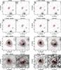 |
Fig. B.2 Deblending of AzTEC-11-N in UltraVista YJHK and Spitzer/IRAC bands. |
Our 1.1 mm-selected sample is based on the SMA follow-up of 15 brightest SMGs drawn from the 1.1 mm AzTEC/JCMT-COSMOS survey at 18′′ angular resolution (AzTEC-1 to AzTEC-15; see Table 1; Younger et al. 2007, 2009). Detailed notes on individual targets are given in Younger et al. (2007, 2009). Here we have extracted the multi-wavelength photometry, tabulated in Table B.1, for the counterparts of these SMGs using the deep COSMOS multi-wavelength catalog, with UltraVista data added. The photometry in the IRAC bands had to be deblended for AzTEC-8 (see Fig. B.1), and that for AzTEC-10 had to specifically be extracted as this source was not present in the catalog (see Younger et al. 2009). The photometry extraction and deblending were performed following the procedure described in detail by Smolčić et al. (2012). Furthermore, AzTEC-11 is a peculiar source that required particular attention. Younger et al. (2009) find that the SMA detection is best fit by a double Gaussian, suggesting a multiple component (N & S) source, labeled AzTEC-11-N and AzTEC-11-S19. They present three positions for this SMG: i) AzTEC-11 when the SMA detection is fit using a single-Gaussian, and ii) AzTEC-11-N and AzTEC-11-S when the SMA detection is fit using a double Gaussian. AzTEC-11 is coincident with an optical/MIR/radio source with a spectroscopic redshift (zspec = 1.599). AzTEC-11-S (which is actually the northern component of the source) cannot be matched to a multi-wavelength counterpart in the deep COSMOS maps. Thus, given the rms in the 20 cm VLA-COSMOS survey we estimate a mm-to-radio based redshift of zmm/radio > 2.58. AzTEC-11-N (which is actually the southern component of the source) has an independent UltraVista and IRAC counterpart. To extract its photometry we have deblended the counterpart of AzTEC-11-N by subtracting a 2D-Gaussian from the maps at the position of the counterpart of AzTEC-11, In Fig. B.2 we show the deblended maps for AzTEC-11-N. We find a photometric redshift of  for this component.
Photometry table for our 1.1 mm-selected sample.
APEX project IDs: 080.A-3056(A), 082.A-0815(A) and 086.A-0749(A).
COSLA-1, COSLA-2, COSLA-3, COSLA-4, COSLA-60, COSLA-73, COSLA-89, and COSLA-158.
If the source is independently detected in various bands then the final false match probability is given by the product of the individual-band false match probabilities.
The fluxes were scaled assuming Sν ∝ ν2 + β where Sν is the flux density at frequency ν and β = 1 the dust emissivity index.
AzTEC-1/COSLA-60, AzTEC-2/COSLA-4, AzTEC-8/COSLA-73, AzTEC-9/COSLA-3, AzTEC-13/COSLA-158.
COSLA-6, COSLA-9, COSLA-11, COSLA-16, COSLA-17, COSLA-23.
COSLA-3, COSLA-5, and COSLA-47.
COSLA-10, COSLA-12, COSLA-48, and COSLA-50.
COSLA-5, COSLA-6, COSLA-8, COSLA-128.
The photometric redshift of AzTEC-5 shows the largest deviation from its spectroscopic redshift, but it is still within 2σ of the (zphot − zspec)/(1 + zspec) distribution (see Fig. 7).
When AzTEC-11 is treated as two separate sources; see Appendix B for details.
COSLA-2, COSLA-3, COSLA-4, COSLA-60, COSLA-73.
A consistent mean redshift ( ) is found if AzTEC-11 is treated as a single source.
COSLA-3, COSLA-4, COSLA-6S, COSLA-17S, COSLA-128.
AzTEC-2, AzTEC-6, AzTEC-9, AzTEC-14W.
COSLA-6-1, COSLA-23-N, COSLA-60, and possibly COSLA-158 with only a lower-redshift limit; see Table 4.
Note that the N & S labels are inverted (see Table 1 in Younger et al. 2009).
Acknowledgments
We thank the anonymous referee for helpful comments on the manuscript. Based on data products from observations made with ESO Telescopes at the La Silla Paranal Observatory under ESO programme ID 179.A-2005 and on data products produced by TERAPIX and the Cambridge Astronomy Survey Unit on behalf of the UltraVISTA consortium. The research leading to these results has received funding from the European Community’s Seventh Framework Programme (/FP7/2007-2013/) under grant agreement No. 229517 and through the DFG-SFB 956 and the DFG Priority Program 1573. The National Radio Astronomy Observatory is a facility of the National Science Foundation operated under cooperative agreement by Associated Universities, Inc.
References
- Alexander, D. M., Bauer, F. E., Chapman, S. C., et al. 2005, ApJ, 632, 736 [NASA ADS] [CrossRef] [Google Scholar]
- Aravena, M., Younger, J. D., Fazio, G. G., et al. 2010a, ApJ, 719, L15 [NASA ADS] [CrossRef] [Google Scholar]
- Aravena, M., Bertoldi, F., Carilli, C., et al. 2010b, ApJ, 708, L36 [NASA ADS] [CrossRef] [Google Scholar]
- Aretxaga, I., Wilson, G. W., Aguilar, E., et al. 2011, MNRAS, 415, 3831 [NASA ADS] [CrossRef] [Google Scholar]
- Banerji, M., Chapman, S. C., Smail, I., et al. 2011, MNRAS, 418, 1071 [NASA ADS] [CrossRef] [Google Scholar]
- Baugh, C. M., Lacey, C. G., Frenk, C. S., et al. 2005, MNRAS, 356, 1191 [NASA ADS] [CrossRef] [Google Scholar]
- Bertoldi, F., Carilli, C., Aravena, M., et al. 2007, ApJS, 172, 132 [NASA ADS] [CrossRef] [Google Scholar]
- Biggs, A. D., Ivison, R. J., Ibar, E., et al. 2011, MNRAS, 413, 2314 [Google Scholar]
- Blain, A. W., Smail, I., Ivison, R. J., Kneib, J.-P., & Frayer, D. T. 2002, PhR, 369, 111 [Google Scholar]
- Blain, A. W., Chapman, S. C., Smail, I., & Ivison, R. 2004, ApJ, 611, 725 [NASA ADS] [CrossRef] [Google Scholar]
- Calzetti, D., Armus, L., Bohlin, R. C., et al. 2000, ApJ, 533, 682 [NASA ADS] [CrossRef] [Google Scholar]
- Capak, P., Aussel, H., Ajiki, M., et al. 2007, ApJS, 172, 99 [NASA ADS] [CrossRef] [Google Scholar]
- Capak, P., Carilli, C. L., Lee, N., et al. 2008, ApJ, 681, L53 [Google Scholar]
- Capak, P. L., Riechers, D., Scoville, N. Z., et al. 2011, Nature, 470, 233 [Google Scholar]
- Carilli, C. L., & Yun, M. S. 1999, ApJ, 513, L13 [NASA ADS] [CrossRef] [Google Scholar]
- Carilli, C. L., & Yun, M. S. 2000, ApJ, 530, 618 [NASA ADS] [CrossRef] [Google Scholar]
- Carilli, C. L., Daddi, E., Riechers, D., et al. 2010, ApJ, 714, 1407 [NASA ADS] [CrossRef] [Google Scholar]
- Carilli, C. L., Hodge, J., Walter, F., et al. 2011, ApJ, 739, L33 [NASA ADS] [CrossRef] [Google Scholar]
- Chapman, S. C., Blain, A. W., Smail, I., & Ivison, R. J. 2005, ApJ, 622, 772 [NASA ADS] [CrossRef] [Google Scholar]
- Chapman, S. C., Neri, R., Bertoldi, F., et al. 2008, ApJ, 689, 889 [NASA ADS] [CrossRef] [Google Scholar]
- Chen, C.-C., Cowie, L. L., Wang, W.-H., Barger, A. J., & Williams, J. P. 2011, ApJ, 733, 64 [NASA ADS] [CrossRef] [Google Scholar]
- Cimatti, A., Cassata, P., Pozzetti, L., et al. 2008, A&A, 482, 21 [NASA ADS] [CrossRef] [EDP Sciences] [Google Scholar]
- Combes, F., Rex, M., Rawle, T. D., et al. 2012, A&A, 538, L4 [NASA ADS] [CrossRef] [EDP Sciences] [Google Scholar]
- Coppin, K. E. K., Smail, I., Alexander, D. M., et al. 2009, MNRAS, 395, 1905 [NASA ADS] [CrossRef] [Google Scholar]
- Coppin, K. E. K., Chapman, S. C., Smail, I., et al. 2010, MNRAS, 407, L103 [NASA ADS] [CrossRef] [Google Scholar]
- Cox, P., Krips, M., Neri, R., et al. 2011, ApJ, 740, 63 [NASA ADS] [CrossRef] [Google Scholar]
- Daddi, E., Dannerbauer, H., Stern, D., et al. 2009a, ApJ, 694, 1517 [Google Scholar]
- Daddi, E., Dannerbauer, H., Krips, M., et al. 2009b, ApJ, 695, L176 [NASA ADS] [CrossRef] [Google Scholar]
- Dannerbauer, H., Lehnert, M. D., Lutz, D., et al. 2002, ApJ, 573, 473 [NASA ADS] [CrossRef] [Google Scholar]
- Downes, D., & Solomon, P. M. 2003, ApJ, 582, 37 [NASA ADS] [CrossRef] [Google Scholar]
- Downes, A. J. B., Peacock, J. A., Savage, A., & Carrie, D. R. 1986, MNRAS, 218, 31 [NASA ADS] [CrossRef] [Google Scholar]
- Downes, D., Neri, R., Greve, A., et al. 1999, A&A, 347, 809 [NASA ADS] [Google Scholar]
- Elvis, M., Civano, F., Vignali, C., et al. 2009, ApJS, 184, 158 [NASA ADS] [CrossRef] [Google Scholar]
- Frayer, D. T., Smail, I., Ivison, R. J., & Scoville, N. Z. 2000, AJ, 120, 1668 [NASA ADS] [CrossRef] [Google Scholar]
- Frayer, D. T., Sanders, D. B., Surace, J. A., et al. 2009, AJ, 138, 1261 [NASA ADS] [CrossRef] [Google Scholar]
- Genzel, R., Baker, A. J., Tacconi, L. J., et al. 2003, ApJ, 584, 633 [NASA ADS] [CrossRef] [Google Scholar]
- Greve, T. R., Bertoldi, F., Smail, I., et al. 2005, MNRAS, 359, 1165 [NASA ADS] [CrossRef] [Google Scholar]
- Hainline, L. J., Blain, A. W., Smail, I., et al. 2009, ApJ, 699, 1610 [NASA ADS] [CrossRef] [Google Scholar]
- Hasinger, G., Cappelluti, N., Brunner, H., et al. 2007, ApJS, 172, 29 [NASA ADS] [CrossRef] [Google Scholar]
- Hatsukade, B., Iono, D., Akiyama, T., et al. 2010, ApJ, 711, 974 [NASA ADS] [CrossRef] [Google Scholar]
- Hayward, C. C., Kereš, D., Jonsson, P., et al. 2011, ApJ, 743, 159 [CrossRef] [Google Scholar]
- Hickox, R. C., Wardlow, J. L., Smail, I., et al. 2012, MNRAS, 421, 184 [Google Scholar]
- Hopkins, P. F., Somerville, R. S., Hernquist, L., et al. 2006, ApJ, 652, 864 [NASA ADS] [CrossRef] [Google Scholar]
- Iglesias-Páramo, J., Buat, V., Hernández-Fernández, J., et al. 2007, ApJ, 670, 279 [NASA ADS] [CrossRef] [Google Scholar]
- Ikarashi, S., Kohno, K., Aguirre, J. E., et al. 2011, MNRAS, 415, 3081 [NASA ADS] [CrossRef] [Google Scholar]
- Ilbert, O., Capak, P., Salvato, M., et al. 2009, ApJ, 690, 1236 [NASA ADS] [CrossRef] [Google Scholar]
- Ivison, R. J., Greve, T. R., Smail, I., et al. 2002, MNRAS, 337, 1 [NASA ADS] [CrossRef] [Google Scholar]
- Ivison, R. J., Smail, I., Dunlop, J. S., et al. 2005, MNRAS, 364, 1025 [NASA ADS] [CrossRef] [Google Scholar]
- Ivison, R. J., Greve, T. R., Dunlop, J. S., et al. 2007, MNRAS, 380, 199 [Google Scholar]
- Iono, D., Peck, A. B., Pope, A., et al. 2006, ApJ, 640, L1 [NASA ADS] [CrossRef] [Google Scholar]
- Kauffmann, G., Heckman, T. M., Tremonti, C., et al. 2003, MNRAS, 346, 1055 [Google Scholar]
- Kneib, J.-P., Neri, R., Smail, I., et al. 2005, A&A, 434, 819 [NASA ADS] [CrossRef] [EDP Sciences] [Google Scholar]
- Knudsen, K. K., Kneib, J.-P., Richard, J., Petitpas, G., & Egami, E. 2010, ApJ, 709, 21 [Google Scholar]
- Koekemoer, A. M., Aussel, H., Calzetti, D., et al. 2007, ApJS, 172, 196 [NASA ADS] [CrossRef] [Google Scholar]
- Leauthaud, A., Massey, R., Kneib, J.-P., et al. 2007, ApJS, 172, 219 [NASA ADS] [CrossRef] [Google Scholar]
- Le Floc’h, E.,Aussel, H., Ilbert, O., et al. 2009, ApJ, 703, 222 [NASA ADS] [CrossRef] [Google Scholar]
- Lilly, S. J., Le Fèvre, O., Renzini, A., et al. 2007, ApJS, 172, 70 [NASA ADS] [CrossRef] [Google Scholar]
- Lilly, S. J., Le Brun, V., Maier, C., et al. 2009, ApJS, 184, 218 [Google Scholar]
- Lindner, R. R., Baker, A. J., Omont, A., et al. 2011, ApJ, 737, 83 [NASA ADS] [CrossRef] [Google Scholar]
- McCracken, H. J., Capak, P., Salvato, M., et al. 2010, ApJ, 708, 202 [NASA ADS] [CrossRef] [Google Scholar]
- McCracken, H. J., Milvang-Jensen, B., Dunlop, J., et al. 2012, A&A, 544, A156 [NASA ADS] [CrossRef] [EDP Sciences] [Google Scholar]
- Menéndez-Delmestre, K., Blain, A. W., Smail, I., et al. 2009, ApJ, 699, 667 [NASA ADS] [CrossRef] [Google Scholar]
- Michałowski, M., Hjorth, J., & Watson, D. 2010, A&A, 514, A67 [NASA ADS] [CrossRef] [EDP Sciences] [Google Scholar]
- Neri, R., Genzel, R., Ivison, R. J., et al. 2003, ApJ, 597, L113 [NASA ADS] [CrossRef] [Google Scholar]
- Pope, A., Borys, C., Scott, D., et al. 2005, MNRAS, 358, 149 [NASA ADS] [CrossRef] [Google Scholar]
- Riechers, D. A., Capak, P. L., Carilli, C. L., et al. 2010, ApJ, 720, L131 [NASA ADS] [CrossRef] [Google Scholar]
- Sanders, D. B., & Mirabel, I. F. 1996, ARA&A, 34, 749 [NASA ADS] [CrossRef] [Google Scholar]
- Sanders, D. B., Salvato, M., Aussel, H., et al. 2007, ApJS, 172, 86 [Google Scholar]
- Sargent, M. T., Schinnerer, E., Murphy, E., et al. 2010, ApJS, 186, 341 [NASA ADS] [CrossRef] [Google Scholar]
- Schinnerer, E., Carilli, C. L., Scoville, N. Z., et al. 2004, AJ, 128, 1974 [NASA ADS] [CrossRef] [Google Scholar]
- Schinnerer, E., Smolčić, V., Carilli, C. L., et al. 2007, ApJS, 172, 46 [NASA ADS] [CrossRef] [Google Scholar]
- Schinnerer, E., Carilli, C. L., Capak, P., et al. 2008, ApJ, 689, L5 [Google Scholar]
- Schinnerer, E., Sargent, M. T., Bondi, M., et al. 2010, ApJS, 188, 384 [NASA ADS] [CrossRef] [Google Scholar]
- Scott, K. S., Austermann, J. E., Perera, T. A., et al. 2008, MNRAS, 385, 2225 [NASA ADS] [CrossRef] [Google Scholar]
- Scoville, N., Aussel, H., Brusa, M., et al. 2007, ApJS, 172, 1 [NASA ADS] [CrossRef] [Google Scholar]
- Sheth, K., Blain, A. W., Kneib, J.-P., et al. 2004, ApJ, 614, L5 [NASA ADS] [CrossRef] [Google Scholar]
- Silva, L., Granato, G. L., Bressan, A., & Danese, L. 1998, ApJ, 509, 103 [NASA ADS] [CrossRef] [Google Scholar]
- Smolčić, V., Capak, P., Ilbert, O., et al. 2011, ApJ, 731, L27 [NASA ADS] [CrossRef] [Google Scholar]
- Smolčić, V., Navarrete, F., Aravena, M., et al. 2012, ApJS, 200, 10 [NASA ADS] [CrossRef] [Google Scholar]
- Swinbank, A. M., Lacey, C. G., Smail, I., et al. 2008, MNRAS, 391, 420 [NASA ADS] [CrossRef] [Google Scholar]
- Tacconi, L. J., Neri, R., Chapman, S. C., et al. 2006, ApJ, 640, 228 [NASA ADS] [CrossRef] [Google Scholar]
- Tamura, Y., Iono, D., Wilner, D. J., et al. 2010, ApJ, 724, 1270 [NASA ADS] [CrossRef] [Google Scholar]
- Taniguchi, Y., Scoville, N., Murayama, T., et al. 2007, ApJS, 172, 9 [NASA ADS] [CrossRef] [Google Scholar]
- Trump, J. R., Impey, C. D., McCarthy, P. J., et al. 2007, ApJS, 172, 383 [NASA ADS] [CrossRef] [Google Scholar]
- van Dokkum, P. G., Franx, M., Kriek, M., et al. 2008, ApJ, 677, L5 [NASA ADS] [CrossRef] [Google Scholar]
- Wall, J. V., Pope, A., & Scott, D. 2008, MNRAS, 383, 435 [NASA ADS] [CrossRef] [Google Scholar]
- Wang, W.-H., Cowie, L. L., Barger, A. J., & Williams, J. P. 2011, ApJ, 726, L18 [NASA ADS] [CrossRef] [Google Scholar]
- Wardlow, J. L., Smail, I., Wilson, G. W., et al. 2010, MNRAS, 401, 2299 [NASA ADS] [CrossRef] [Google Scholar]
- Wardlow, J. L., Smail, I., Coppin, K. E. K., et al. 2011, MNRAS, 415, 1479 [NASA ADS] [CrossRef] [Google Scholar]
- Younger, J. D., Fazio, G. G., Huang, J.-S., et al. 2007, ApJ, 671, 1531 [Google Scholar]
- Younger, J. D., Fazio, G. G., Wilner, D. J., et al. 2008, ApJ, 688, 59 [NASA ADS] [CrossRef] [Google Scholar]
- Younger, J. D., Fazio, G. G., Huang, J.-S., et al. 2009, ApJ, 704, 803 [NASA ADS] [CrossRef] [Google Scholar]
- Yun, M. S., Aretxaga, I., Ashby, M. L. N., et al. 2008, MNRAS, 389, 333 [NASA ADS] [CrossRef] [Google Scholar]
- Yun, M. S., Scott, K. S., Guo, Y., et al. 2012, MNRAS, 420, 957 [NASA ADS] [CrossRef] [Google Scholar]
- Zamojski, M. A., Schiminovich, D., Rich, R. M., et al. 2007, ApJS, 172, 468 [NASA ADS] [CrossRef] [Google Scholar]
All Tables
Statistical samples of SMGs with ≲2′′ angular resolution mm-detections in the COSMOS field.
LABOCA sources observed with mm-interferometers at ≲2′′ resolution, and with counterparts identified via P-statistic.
AzTEC/JCMT/SMA SMGs with identified robust/tentative counterparts based on the P-statistics.
All Figures
|
Fig. 1 Distribution of separations between the PdBI sources and the corresponding LABOCA-COSMOS sources. |
| In the text | |
|
Fig. 2 Comparison between LABOCA 870 μm and PdBI 1.3 mm fluxes for SMGs (indicated in the panel) detected (middle panel) and not detected (top panel) with the PdBI. For LABOCA sources identified as multiple PdBI sources the individual PdBI source fluxes were added, and for the LABOCA sources not detected by PdBI 1.3 mm flux estimates for the most likely multi-wavelength counterparts were extracted from the PdBI maps (see Sect. 3.3 for details). The bottom panel shows the comparison between AzTEC 1.1 mm and SMA 890 μm fluxes (adopted from Younger et al. 2007, 2009) for AzTEC/JCMT SMGs in our 1.1 mm-selected sample. The solid line in all panels shows the flux ratios for a spectral power law index of 3. |
| In the text | |
|
Fig. 3 3.6 μm, 24 μm, and 20 cm stamps (30′′ × 30′′ area) for LABOCA COSMOS sources detected by mm-interferometers at ≲2′′ resolution (see Table 3). The bands and sources are indicated in the panels and the names of sources detected with interferometers at S/N > 4.5 are underlined. The thick yellow circle, 2′′ in diameter, indicates the mm-interferometer position. Robust (square) and tentative (diamond) counterparts determined via P-statistic in each particular (3.6 μm, 24 μm, and 20 cm) band are also shown (see text for details; see also Table 6). For each source LABOCA contours in 1σ steps starting at 2σ (with locally determined rms) are overlaid onto the 3.6 μm stamp. |
| In the text | |
|
Fig. 3 continued. |
| In the text | |
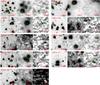 |
Fig. 4 Same as Fig. 3 but for LABOCA sources not detected within our PdBI observations. |
| In the text | |
|
Fig. 5 Same as Fig. 3, but for AzTEC/JCMT/SMA COSMOS sources in our 1.1 mm-selected sample (see Tables 1 and 7). The AzTEC/JCMT beam is indicated by the circle in the 3.6 μm stamp. |
| In the text | |
|
Fig. 6 Photometric redshift total χ2 distributions for our SMGs with spectroscopic redshifts. We show results based on various sets of spectral models (see text for details): 2T (dotted lines), 6T (dashed-lines), M (full lines). The spectroscopic redshifts are indicated by vertical dashed lines. The source names and the number of degrees of freedom (dof) in the photometric redshift χ2 minimization are indicated in each panel. The gray-shaded areas in some of the panels indicate the redshift range ignored for the determination of the best-fit photometric redshift. The photometric redshift provided by the best model (M) and its uncertainty was taken as the minimum χ2 value and the 99% confidence interval, respectively, both indicated in each panel by the thick and thin red lines. |
| In the text | |
|
Fig. 7 Comparison of spectroscopic and photometric redshifts for 16 starbursts in our COSMOS sample. The photometric redshifts were determined using the Michalowski spectral templates, and the shown errors are ± 3σ errors drawn from the χ2 distributions of the photometric-redshift fits (see Fig. 6 and text for details). The median offset and standard deviation of the Δz/(1 + zspec) distribution are indicated in the bottom panel. Note that for z ≥ 3 we find a slight, 0.04·(1 + z), systematic underestimate of the photometric redshifts. |
| In the text | |
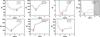 |
Fig. 8 Same as Fig. 6, but for our AzTEC/JCMT/SMA COSMOS SMGs without spectroscopic redshifts. |
| In the text | |
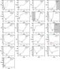 |
Fig. 9 Same as Fig. 6, but for our LABOCA/PdBI COSMOS SMGs without spectroscopic redshifts. |
| In the text | |
|
Fig. 10 Redshift distribution of our 1.1 mm-selected sample (left panel), 870 μm-selected sample (middle panel), and the two samples combined (with sources present in both samples counted only once; right panel). In the middle panel we also show the redshift distribution of our S/N1.1 mm > 4.5 PdBI-detected LABOCA sample (hatched histogram). Mean redshift values, and corresponding errors obtained using the statistical package ASURV, as well as the number of sources in each sample are indicated in each panel. Mean redshifts for every sample distribution are also indicated by the thick vertical lines. |
| In the text | |
|
Fig. 11 Normalized redshift distributions for SMGs drawn from various studies in the literature, indicated in the panel. |
| In the text | |
|
Fig. A.1 Optical to radio stamps for the LABOCA-COSMOS SMGs detected by PdBI. Names of sources with S/N > 4.5 in PdBI maps are underlined. |
| In the text | |
|
Fig. A.1 continued. |
| In the text | |
|
Fig. A.1 continued. |
| In the text | |
|
Fig. A.2 Cleaned PdBI maps (color scale), 30′′ on the side, with ± 2σ,3σ,... contours overlaid. Detections (identified in the dirty maps, see text for details) are marked by crosses. |
| In the text | |
|
Fig. B.1 Deblending of AzTEC-8 in Spitzer/IRAC bands. |
| In the text | |
|
Fig. B.2 Deblending of AzTEC-11-N in UltraVista YJHK and Spitzer/IRAC bands. |
| In the text | |
Current usage metrics show cumulative count of Article Views (full-text article views including HTML views, PDF and ePub downloads, according to the available data) and Abstracts Views on Vision4Press platform.
Data correspond to usage on the plateform after 2015. The current usage metrics is available 48-96 hours after online publication and is updated daily on week days.
Initial download of the metrics may take a while.