| Issue |
A&A
Volume 550, February 2013
|
|
|---|---|---|
| Article Number | A6 | |
| Number of page(s) | 8 | |
| Section | The Sun | |
| DOI | https://doi.org/10.1051/0004-6361/201015215 | |
| Published online | 17 January 2013 | |
The chaotic solar cycle
II. Analysis of cosmogenic 10Be data
1 Inst. für Physik, Geophysik Astrophysik und Meteorologie, Univ.-Platz 5, 8010 Graz, Austria
e-mail: This email address is being protected from spambots. You need JavaScript enabled to view it.
2 Hvar Observatory, Faculty of Geodesy, University of Zagreb, Kačićeva 26, 10000 Zagreb, Croatia
e-mail: This email address is being protected from spambots. You need JavaScript enabled to view it.
; This email address is being protected from spambots. You need JavaScript enabled to view it.
; This email address is being protected from spambots. You need JavaScript enabled to view it.
; This email address is being protected from spambots. You need JavaScript enabled to view it.
;
3 Eawag, Swiss Federal Institute of Aquatic Science and Technology, Überlandstrasse 133, 8600 Dübendorf, Switzerland
e-mail: This email address is being protected from spambots. You need JavaScript enabled to view it.
4 Department of Astronomy, University of Washington, PO Box 351580, Seattle, WA 98195, USA
e-mail: This email address is being protected from spambots. You need JavaScript enabled to view it.
; This email address is being protected from spambots. You need JavaScript enabled to view it.
5 Department of Physics, University of Zagreb, Bijenička c. 32, PP 331, 10000 Zagreb, Croatia
6 Cybrotech Ltd., Bohinjska 11, 10000 Zagreb, Croatia
e-mail: This email address is being protected from spambots. You need JavaScript enabled to view it.
Received: 15 June 2010
Accepted: 14 September 2012
Abstract
Context. The variations of solar activity over long time intervals using a solar activity reconstruction based on the cosmogenic radionuclide 10Be measured in polar ice cores are studied.
Aims. The periodicity of the solar activity cycle is studied. The solar activity cycle is governed by a complex dynamo mechanism. Methods of nonlinear dynamics enable us to learn more about the regular and chaotic behavior of solar activity. In this work we compare our earlier findings based on 14C data with the results obtained using 10Be data.
Methods. By applying methods of nonlinear dynamics, the solar activity cycle is studied using solar activity proxies that have been reaching into the past for over 9300 years. The complexity of the system is expressed by several parameters of nonlinear dynamics, such as embedding dimension or false nearest neighbors, and the method of delay coordinates is applied to the time series. We also fit a damped random walk model, which accurately describes the variability of quasars, to the solar 10Be data and investigate the corresponding power spectral distribution. The periods in the data series were searched by the Fourier and wavelet analyses.
Results. The solar activity on the long-term scale is found to be on the edge of chaotic behavior. This can explain the observed intermittent period of longer lasting solar activity minima. Filtering the data by eliminating variations below a certain period (the periods of 380 yr and 57 yr were used) yields a far more regular behavior of solar activity. A comparison between the results for the 10Be data with the 14C data shows many similarities. Both cosmogenic isotopes are strongly correlated mutually and with solar activity. Finally, we find that a series of damped random walk models provides a good fit to the 10Be data with a fixed characteristic time scale of 1000 years, which is roughly consistent with the quasi-periods found by the Fourier and wavelet analyses.
Conclusions. The time series of solar activity proxies used here clearly shows that solar activity behaves differently from random data. The unfiltered data exhibit a complex dynamics that becomes more regular when filtering the data. The results indicate that solar activity proxies are also influenced by other than solar variations and reflect solar activity only on longer time scales.
Key words: solar-terrestrial relations / Sun: activity / Sun: general
© ESO, 2013
1. Introduction
The study of the periodic, chaotic, or stochastic nature of solar activity requires the analysis of long-lasting time series of solar activity indices. Since direct solar activity observations have been available only since the beginning of telescopic observations and cover a time span of several hundred years, proxies of solar activity have to be used. Such proxies could be observations of aurorae, cosmogenic isotopes, growth of certain plants like corals, etc. They have to be used to obtain a longer time series of the solar activity. An overview of these proxies can be found, e.g., in Hanslmeier (2007).
The theory of deterministic chaos has been successfully applied to many areas of physics, including geophysics, astrophysics, and meteorology (Peitgen et al. 1994, 2004; Cvitanović et al. 2009). Chaotic phenomena in astrophysics and cosmology, mainly for dynamics in the solar system and galactic dynamics as well as for such applications to cosmology as properties of cosmic microwave background radiation, were reviewed by Gurzadyan (2002), while the phenomena showing evidence of nonlinear dynamics in solar physics are summarized by Wilson (1994) and by Hanslmeier (1997).
The main motivation for this work is to address the question whether solar behavior is chaotic or random. The answer to this question is important for at least two reasons. First, it has implications for the dynamo models, which according to present ideas should describe the physical processes that govern the observed manifestations of solar magnetic activity. Second, this distinction is important for procedures of predicting and reconstructing solar activity on different temporal scales.
Chaos is a special kind of complex behavior of dynamic systems described by nonlinear equations. The dynamic variables that describe the properties of the system and its time evolution are in the nonlinear form, i.e., they have higher order terms. Indications of chaotic behavior in solar dynamo models are present in a number of cases. The solar activity cycle is modulated by several quasi-periodic cycles showing period-doubling characteristics and aperiodic grand minima with a characteristic time scale exceeding several tens of cycle periods (Ruzmaikin et al. 1992; Rüdiger & Hollerbach 2004). The impossibility of representing long-term sunspot cycle as a periodic process, period-doubling oscillations, and positive Kolmogorov entropy found in 14C data (Gizzatullina et al. 1990) point to deterministic chaos (Ruzmaikin et al. 1992). Possible mechanisms include (i) nonlinear back-reaction of the magnetic field visible in a modulation of the differential rotation; (ii) stochastic fluctuation of the α-effect; (iii) variation in the meridional circulation; (iv) on-off intermittency due to a threshold field strength for dynamo action. Nonlinearity is present in equations of motion, where the Lorenz force is quadratic in a magnetic field, and possibly in dynamo equations, where α may also be quadratic in a magnetic field (Hoyng 1992; Rosner & Weiss 1992; Stix 2002; Mestel 2003; Ossendrijver 2003; Schüssler & Schmitt 2004).
This paper is a continuation of our study about the chaotic solar cycle using 14C measurements (Hanslmeier & Brajša 2010), which is referred to as Paper I in this work. In Paper I, references to studies of nonlinear effects in the solar activity in theoretical models are given. In addition, fluctuations in solar dynamo parameters were considered to explain variability of the solar cycle (Hoyng 1993; Ossendrijver & Hoyng 1996; Moss et al. 2008). Chaos and intermittency in the solar cycle were reviewed by Spiegel (2009).
Nonlinear dynamics methods have also been applied to predicting solar activity cycles (see, e.g., Sello 2001; Aguirre et al. 2008; Kitiashvili & Kosovichev 2008), and one has to distinguish between stochastic and chaotic behavior. The reader is again referred to the literature cited in Paper I.
Steinhilber et al. (2008) used the results of Vonmoos et al. (2006) and reconstructed solar activity for about the past 9300 years using the cosmogenic radionuclide 10Be measured in polar ice cores. In that paper, solar activity is expressed as solar modulation potential Φ. This Φ record has been used recently to obtain other records of solar activity, such as interplanetary magnetic field (Steinhilber et al. 2010) and total solar irradiance (Steinhilber et al. 2009). The abundance depends on the intensity of the cosmic ray flux, which can enter the Earth’s atmosphere. The intensity of cosmic rays is lower when the Sun is very active and vice versa. Thus, there is an anticorrelation between the production of cosmogenic isotopes and solar activity. Besides solar activity, the 10Be signal is also influenced by geomagnetic field intensity variations and system (climate) effects. However, when the data is averaged over 22 or more years, the system effect component contributes less than 10% to the total signal (McCracken 2004). We note that in Vonmoos et al. (2006) and in Steinhilber et al. (2008) the effect by geomagnetic field intensity variations has already been considered. However, there is large uncertainty in the reconstructions of geomagnetic field intensity. In addition, because the geomagnetic field intensity has to be considered when using cosmogenic radionuclides (e.g., 10Be, 14C), there is also some uncertainty in the Φ reconstruction. To estimate geomagnetic influence, we follow the same approach as in Paper I and add random noise with different amplitudes to the Φ record.
While the usual, well-known random walk model has been widely used in solar physics (e.g., Leighton 1964; Sheeley et al. 1987; Wang & Sheeley 1994; Hagenaar et al. 1999; Hathaway 2005; Brajša et al. 2008), this is not the case with the damped random walk (DRW) model. In the present work, we use a DRW model to analyze the time series of reconstructed solar activity.
In a non-solar context, Kelly et al. (2009) introduced a model where the optical variability of a given quasar is described by a DRW. The difference with respect to the well-known random walk is that an additional self-correcting term pushes any deviations back towards the mean flux on a time scale τ. It has been established by Kelly et al. (2009), Kozłowski et al. (2010), and MacLeod et al. (2010) that a DRW can statistically explain the observed light curves of quasars at an impressive fidelity level (0.01−0.02 mag). The model has only three free parameters: the mean value of the light curve (μ), the driving amplitude of the stochastic process, and the damping (or characteristic) time scale τ. The predictions are only statistical, and the random nature reflects our uncertainty about the details of the physical processes.
The paper is structured as follows. In Sect. 2, the data and the applied method to analyze the data are described. Section 3 gives the results, and in Sect. 4, we summarize our main results and draw the conclusions.
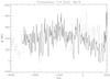 |
Fig. 1 Time series of reconstructed solar activity (Φ) based on 14C (full line) and 10Be measurements (dotted line). Years are given in calendar AD years. The data points correspond to centers of the 25-year intervals. Negative values on the y-axis are artifacts and are consistent with zero within the error limits due to uncertainty in measuring 10Be and in geomagnetic field intensity. |
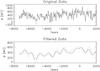 |
Fig. 2 Time series of solar activity (Φ) based on 10Be measured in polar ice cores for the past 9300 years. On the upper plot are the original data, while on the lower plot, the Fourier-filtered data are shown. Fluctuations at periods for t ≤ 380 yr (full line) were suppressed by a Fourier filter. To simulate geomagnetic field-strength variation, a random signal of similar amplitude to the original signal and a period of about 760 years were added (same approach as in Paper I) (dotted line). |
2. Data and data analysis
2.1. Data
The solar modulation function Φ during most of the Holocene (last 9300 years) was reconstructed based on the cosmogenic 10Be data, as described by Vonmoos et al. (2006) and by Steinhilber et al. (2008). The data used, which were analyzed by different methods of nonlinear dynamics, are shown in Figs. 1 and 2. The 10Be data are limited to the last 9300 years due to some missing measurements corresponding to the time prior to that period. Also, a climatic change occurred at the end of the last glacial period about 11 700 years ago. Such climatic changes could be connected to the change in the precipitation rate and thus to the 10Be concentration in ice (system effects). However, during the Holocene period, there are no indications for strong changes in the precipitation source for central Greenland (Johnsen et al. 1989; Mayewski et al. 1997).
As stated in the Introduction, the variations seen in the data should be due to changes in solar activity. However, even though the data are filtered, there could be still some influence/error due to system effects (climate) and uncertainty in the reconstructions of geomagnetic field intensity. To test the robustness of our results, we followed our approach in Paper I, i.e., stimulating the field by adding random data of different amplitudes to the original values and then studying how the results changed.
2.2. Methods of nonlinear dynamics and time series analysis
We present the calculation of the same parameters that were studied in Paper I:
-
mutual information;
-
embedding dimension;
-
false nearest neighbors.
For a more detailed description of these parameters, see Paper I or the papers by Takens (1980), Sauer et al. (1991), Kennel et al. (1992), Kantz & Schreiber (1997), Rhodes & Morari (1997), and Schreiber (1999). The method of delayed coordinates (also described in Paper I) was used for the 10Be data, and a comparison with the 14C data is given.
2.3. Damped random walk
The time variability is modeled as a stochastic process described by the exponential covariance matrix 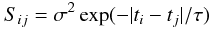 (1)between times ti and tj. As explained by Kelly et al. (2009) and Kozłowski et al. (2010), this corresponds to a DRW with a damping, or characteristic time scale τ and a long-term standard deviation of variability σ. The DRW model used here is more specifically an Ornstein-Uhlenbeck process. Following Kozłowski et al. (2010), we model the time series of solar activity and estimate the parameters and their uncertainties using the method of Press et al. (1992), its generalization in Rybicki & Press (1992), and the fast computational implementation described in Rybicki & Press (1995). As in MacLeod et al. (2010), we express the long-term variability in terms of the structure function (SF), where the SF is the root mean square (rms) magnitude difference as a function of the time lag (Δt) between measurements. The characteristic time scale for the SF to reach an asymptotic value SF∞ is the damping time scale, τ. The SF for a DRW is
 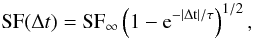 (2)and the asymptotic value at large Δt is
  (3)In addition to the χ2 per degree of freedom (χ2/Nd.o.f.), information on the goodness of fit is provided by the parameters ΔLnoise and ΔL∞. We define ΔLnoise ≡ ln(Lbest/Lnoise), which was used in Kozłowski et al. (2010) and MacLeod et al. (2010) to select quasar light curves that are better described by a DRW than by pure white noise. Here, Lbest is the likelihood of the best-fit stochastic model and Lnoise is that for a white noise solution (τ ≡ 0). We define ΔL∞ ≡ ln(Lbest/L∞), where L∞ is the likelihood that τ → ∞, indicating that the length of the time series under consideration is too short to accurately measure τ.
2.4. Period analysis
To find out if there was some periodicity in the analyzed time series, we applied the Fourier analysis according to the method of Deeming (1975) and its’ later upgraded version of Lenz & Breger (2005). Furthermore, we used the wavelet analysis of Torrence & Compo (1998). This method made it possible to identify especially pronounced quasi-periods (see, e.g., Temmer et al. 2004).
3. Results
First we give a comparison between the 14C and 10Be measurements (Fig. 1). The carbon measurements give the reconstructed sunspot index; these values were scaled to the Φ measurements from the 10Be data as earlier described. It is seen that the general trend of the data is quite similar, in agreement with Beer et al. (2007) and Usoskin et al. (2009). The 14C data are sampled every ten years, the 10Be data every 25 years.
3.1. Nonlinear dynamics
In the upper panel of Fig. 2, the reconstructed Φ record is shown. To suppress noise, a Fourier filter of 380 years was applied to eliminate the shorter time scale fluctuations seen in the data shown in the lower panel in Fig. 2.
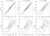 |
Fig. 3 Delayed coordinates for the 14C data. For a discussion, see Sect. 3.1. |
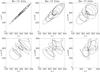 |
Fig. 4 Delayed coordinates for the 10Be data. For a discussion, see Sect. 3.1. |
We simulated a possible variation in the geomagnetic field to demonstrate the robustness of the results. In Fig. 2 results are also shown for a simulation of random geomagnetic variations of a period twice the filtering period of 380 years (dotted line). The amplitudes were chosen to simulate a worst case, which means they are of comparable amplitude to the original data. These assumptions correspond to statements by Solanki et al. (2004, Fig. 3c), who reported a magnetic dipole variation of a factor of two at the maximum and of a period that is at least longer than the value used for our filtered data.
Next, the delay method was applied. This method is also based on the theorem of Takens (1980) and Sauer et al. (1991). More details on this method can be found in Paper I. In Figs. 3 and 4, a study of delayed data for the 14C and the 10Be is given. The delay values were taken as Δt = 1,5,10,15,25, which means the data values xi are plotted versus xiΔt. We note that the value of Δt = 1 means a time gap of 10 yr in the case of the 14C data and 25 yr in the case of the 10Be data. Since we only want to demonstrate the chaotic or nonchaotic behavior for the given data sets, this difference does not have any significance here. The results shown are for the filtered data, which distinctly show some regular behavior. The results given in Figs. 3 and 4 clearly demonstrated that the dynamics becomes more complex when going to variations on a shorter time scale. The behavior of the attractor given by the delay coordinates does not show a significant difference with respect to the original filtered data. By such a filter, variations below a time scale of 57 years were eliminated (not shown here).
In Fig. 5 the mutual information is shown as a function of delay (upper panel) and the false nearest neighbors (lower panel) for the the different datasets: unfiltered data (full line), filtered data (dotted line), and random data (dashed line). For the filtered data, the mutual information curve decreases less steeply than for the original data. For the random data, the graph immediately declines to zero.
To investigate what effect the length of the time series could have on the results, we split the 10Be data into two halves and compare the results for each dataset (Figs. 6 and 7). The results concerning false nearest neighbor and mutual information were found to be quite similar. Therefore, our results are not influenced by the limits of the available time series.
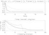 |
Fig. 5 Mutual information as a function of delay and false nearest neighbors for unfiltered data (full line), filtered data (dotted line), and random data (dashed line). |
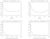 |
Fig. 6 Mutual information as a function of delay and false nearest neighbors for two halves of the filtered 10Be dataset. Left-handed (right-handed) plots refer to the first (second) subset of the data. |
Best-fit DRW parameters for solar 10Be data.
3.2. Damped random walk
Table 1 lists the best-fit DRW parameters for the solar 10Be data, assuming an uncertainty of 80 megavolts (MV) for all data points. A relative likelihood of ΔLnoise = 29 indicates that the best-fit DRW model provides a better fit to the 10Be data than pure white noise. However, a single DRW model cannot accurately reproduce the data and yields a reduced χ2 of 1.9. A series of DRW models with τ fixed to 1000 years and varying SF∞ produces an average model that is in perfect agreement with the data to within the adopted errors, whereas a series of DRW models with varying τ and fixed SF∞ = 165 MV cannot reproduce the data. Therefore, the best-fit characteristic time scale of 1000 years seems to be well constrained. However, we note that the time scale of 1000 years has a large uncertainty when measured using a DRW analysis due to the limited light curve length for the solar data. The best-fit DRW model gives 1σ Bayesian upper and lower limits on τ of 104.4 and 102.9 years, respectively. The data and best-fit DRW models are shown in Fig. 8.
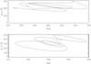 |
Fig. 7 Delayed coordinates for two halves of the 10Be dataset. Upper (lower) plot referes to the first (second) subset of the data. |
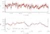 |
Fig. 8 Top panel: entire time series for the solar 10Be data. Data points with error bars show the observed data. The solid line shows the weighted average of all consistent DRW models with τ = 1000 years (SF∞ is allowed to vary from model to model). Dotted lines show the ± 1σ range of these possible stochastic models about the average. Bottom panel: zoomed-in segment of the time series. |
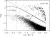 |
Fig. 9 PSD comparison of the solar 10Be data (large dots) and a DRW model (smaller dots) with τ = 1000 years (indicated by the dotted line). A DRW process has a spectral index of − 2 on short time scales (shown by the dashed line), which is shallower than that for the 10Be data on short time scales. The dotted-dashed line shows the average PSD for many DRW models with τ = 1000 years. |
The inability of a single DRW process to describe the solar 10Be data is due to an inaccurate power spectral distribution (PSD) description on short time scales. In Fig. 9, the PSD for the solar 10Be data is compared to the PSD for a DRW model. The x-axis is log frequency in [1/years]. The y axis has arbitrary units. The smaller dots show the PSD for a DRW process with a characteristic time scale arbitrarily set to τ = 102.7 years (indicated by the vertical dotted line), and the larger dots show the PSD for the solar 10Be data. The dashed line shows a spectral index of −2, which corresponds to a DRW process on time scales shorter than τ. However, the solar data show a steeper PSD slope than a DRW at frequencies larger than about 10-0.1 yr-1. The dotted-dashed line shows the average PSD for many DRW models with τ = 1000 years, which is still too shallow to accurately describe the solar data. This discrepancy between the data and DRW models can be seen in Fig. 8, where some of the observed points fall outside of the 1σ range of model light curves (shown as dotted lines), but the data are still consistent with the models, given their uncertainty of 80 MV. In other words, the data generally show a larger scatter on short time scales with respect to the DRW model.
3.3. Period analysis
The solar 10Be time series was also analyzed by Period04 software (Lenz & Breger 2005). Table 2 lists several strongest quasi-periods as seen in Fourier spectrum (Fig. 10) with a dominant approximatively 1000-year cycle. The wavelet analysis results obtained are presented in Fig. 11. We see that by applying the wavelet analysis a quasi-period of about 1000 yr can also be identified, but the significance is not very high and varies during the analyzed time interval.
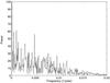 |
Fig. 10 Fourier spectrum for solar 10Be data. |
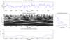 |
Fig. 11 Wavelet analysis of the solar 10Be data using the Morlet wavelet. a) Time series of solar modulation function (Φ) anomalies from unfiltered 10Be data. b) Wavelet power spectrum: darker contours indicate the higher values of wavelet power. White thin line is the cone of influence, below which edge effects become important. c) Global wavelet power spectrum, i.e., the temporal mean wavelet power at each period. Dashed line is the 95% confidence level. d) Scale-averaged time series for the period band 800 − 1200 years. Dashed line is the 95% confidence level. For more information about wavelet analysis, see Torrence & Compo (1998). |
4. Discussion and conclusions
We applied standard methods of nonlinear dynamics (the time series analysis including calculation of the embedding dimension and delay, the false nearest neighbor estimation, and the investigation of the mutual information; for details see Paper I) to study the behavior of solar activity. It must be stressed that the data consist of averaged values, where the averaging was done over a 25-year interval. Therefore, the results are only indicative of longer term variations and do not include and represent the 11-year solar activity cycle because of the short-term noise and limited sampling rate in the 10Be data. Hence, the conclusions are valid for longer time scale modulations of solar activity. To make a further distinction between shorter time scale and longer time scale variations, we applied a Fourier low-pass filtering.
The mutual information and false nearest neighbor methods applied give insight into the complexity of the underlying system. From this information, we estimated the embedding dimension m. In the case of the unfiltered data, we obtained the value m = 15. At this value, the number of false nearest neighbors becomes very small (Fig. 5). In the case of filtered data, this value is lower, while for the elimination of fluctuations with t ≤ 380 yr, the value is about five. Both values are similar to the values obtained in Paper I. The complexity of the system therefore strongly increases on shorter time scales.
Also, we repeated the method of delay coordinates for different delay values. The results for the 10Be data are similar to the ones obtained with the 14C data (see Paper I). The topological structure is quite complex when considering the unfiltered original data. The structure, however, becomes fairly simple when considering the filtered data, eliminating t ≤ 380 yr fluctuations.This can be interpreted that solar activity proxies seem to exhibit a more regular and predictable behavior when variations at larger time scales are considered. These larger time scales are well above 100 years.
Concerning the methods of nonlinear dynamics, we have analyzed the time series, estimated the false nearest neighbors, and calculated the mutual information. The mutual information is a generalization of the autocorrelation function. Also, the method of delays and the calculation of the embedding dimension m were applied. The embedding dimension can help to answer the question whether the topological structure of a system in a phase space is preserved by transformation (mapping). The topological structure is preserved if neighbors are mapped into neighbors, and it is not preserved if this is not the case. Moreover, it is well known that the Lyapunov exponents determine the evolution of a dynamical system.
The topological structure of a system is preserved if m > m0, and it is not preserved if m < m0, where m0 is the minimal embedding dimension for a time series. In that last case, the neighbors are mapped into false neighbors.
For the data used in the present analysis, we can estimate the value of m0 from the upper panel of Fig. 5 (mutual information as a function of delay). All curves become fairly constant at the y-value of about one or less. As a result, m0 = 1. Now from the lower panel of Fig. 5 (fraction of false nearest neighbors as a function of m), we can estimate m for the unfiltered and filtered data. For the unfiltered data, m = 15, and for filtered data, m has a smaller value of 7. So we can conclude that the criterion m > m0 holds for both the filtered and the unfiltered data, implying that the topological structure is preserved, i.e., that the neighbors are fairly well mapped into neighbors after the transformation.
The application of false nearest neighbors and embedding dimension in the astrophysical (and especially in the solar context) are discussed in detail by Regev (2006) and by Gilmore & Letellier (2007). In order to test our analysis against the dependence on the number of data points used, we split the 10Be data into two halves and compared the results for each subset. As the results are quite similar, we conclude that they are not influenced by those limits.
Finally, we fit a DRW model, which accurately describes the variability of quasars, to the solar 10Be data. In this way, we find that a series of DRW models provides a good fit to the 10Be data with a characteristic time scale of 1000 years.
The best-fit τ from the DRW analysis (1000 years) seems to be real, although the power spectrum of the solar 10Be data has a different shape than that for a DRW process (the latter has a shallower power-law slope). Although the DRW process is linear and stochastic, this does not necessarily mean that the solar 10Be data are not consistent with a chaotic, nonlinear, and deterministic process, even if the data were perfectly described by the DRW model. Stochastic processes are commonly used to approximate an astrophysical time series that is truly chaotic in nature, and our analysis in Sect. 2.3. may indeed represent a similar approximation.
In addition, we note that Ma (2007) found a 1000-year cycle in solar activity by investigating long-term fluctuations of reconstructed sunspot number series. It is interesting that a quasi-period of about 1000 years was also identified in the present work using Fourier and wavelet analyses, though there were equally strong quasi-periods at 207 and 2169 years. Concerning the influence of geomagnetic field variations, one can estimate that variations on a time scale of the order of 1 ky are of solar origin, but longer periodicities > 3 ky may be caused by magnetic modulation.
Our results on the stochastic and chaotic properties of solar activity based on 10Be data are quite similar to the results obtained with the 14C time series discussed in Paper I, confirming the findings of Beer et al. (2007) and of Usoskin et al. (2009). This demonstrates the robustness of our method and indicates that such an analysis tool is suited to study the complex time behavior of such systems. Both cosmogenic isotopes are strongly correlated mutually and with solar activity.
The cosmogenic radionuclides 14C and 10Be as long-term indices for solar activity were studied by Beer (2000a,b) and Steinhilber et al. (2008). They stress that these data are produced in a similar way, but that their geochemical behavior is different. The 10Be production rate (0.018 cm-2 s-1) is more than 100 times lower than that of 14C because it is only produced by high-energy spallation processes, where 14C is produced by thermal neutrons interacting with nitrogen. After production, 10Be gets attached to aerosols and is immediately removed from the atmosphere after about one year. It is then transported to the ground, where it is archived, e.g., in polar ice. In contrast, 14C after production forms 14CO2 and is included in the global carbon cycle, i.e., it is exchanged between the reservoirs of CO2, such as atmosphere, biosphere, and the oceans. Consequently, it has much longer residence times, depending on the reservoir (atmosphere: ten years; biosphere: 60 years; ocean: 1000 years).
Thus, the 14C signal (called Δ 14C) is not the 14C production rate at one timepoint, but reflects the 14C production integrated over several millennia. In addition, one has to consider that the halflife of 14C is about 5730 years, which is of the same order as the exchange processes between atmosphere, biosphere, and the ocean. As a result, the carbon cycle and the radioactive decay of 14C have to be considered in order to get the 14C production rate out from the Δ 14C. Both have been considered in Solanki et al. (2004), whose record was the basis for Paper I.
The carbon cycle itself has no influence on the transport of 10Be to the polar ice, and thus we can conclude here that the similarities we found between these two radionuclides indicate that the dominant signal in the data is the production signal due to solar activity and geomagnetic field intensity variations rather than a climate signal. Our findings agree with the study by Beer et al. (2007), who applied principal component analysis to both radionuclides. They found that most of the variation is described by the first principal component, which reflects production. In a continuation of this work, we plan to perform the Hurst analysis of the 14C and 10Be data.
Acknowledgments
The research leading to the results presented in this paper received partial funding from the European Community’s Seventh Framework Programme (FP7/2007 − 2013) under grant agreements nos. 218816 (SOTERIA) and 263252 (COMESEP) and from the Alexander von Humboldt Foundation. F. Steinhilber acknowledges financial support by NCCR Climate – Swiss climate research. Ž. Ivezić acknowledges support by the Croatian National Science Foundation grant O-1548-2009. The authors also acknowledge the support from the Austrian-Croatian Bilateral Scientific Project (2010/11) for financing the exchange of scientists and would like to thank B. Kelly for helpful insight regarding the DRW process as well as J. Beer and the anonymous referee for helpful comments and suggestions.
References
- Aguirre, L. A., Letellier, C., & Maquet, J. 2008, Sol. Phys., 249, 103 [NASA ADS] [CrossRef] [Google Scholar]
- Beer, J. 2000a, SSRV, 93, 107 [Google Scholar]
- Beer, J. 2000b, SSRV, 94, 53 [Google Scholar]
- Beer, J., McCracken, K. G., Abreu, J., Heikkilä, U., & Steinhilber, F. 2007, Proc. 30th Int. Cosmic Ray Conf., Merida, Mexico [Google Scholar]
- Brajša, R., Wöhl, H., Vrnak, B., et al. 2008, Cent. Eur. Astrophys. Bull., 32, 165 [NASA ADS] [Google Scholar]
- Cvitanović, P., Artuso, R., Mainieri, R., Tanner, G., & Vattay, G. 2009, Chaos: Classical and Quantum, ChaosBook.org [Google Scholar]
- Deeming, T. J. 1975, Ap&SS, 36, 137 [NASA ADS] [CrossRef] [MathSciNet] [Google Scholar]
- Gilmore, R., & Letellier, C. 2007, The Symmetry of Chaos (New York: Oxford University Press) [Google Scholar]
- Gizzatullina, S. M., Rukavishnikov, V. D., Ruzmaikin, A. A., & Tavastsherna, K. S. 1990, Sol. Phys., 127, 281 [NASA ADS] [CrossRef] [Google Scholar]
- Gurzadyan, V. G. 2002, in The Ninth Marcel Grossmann Meeting, eds. V. G. Gurzadyan, R. T. Jantzen, & R. Ruffini, 182 [Google Scholar]
- Hagenaar, H. J., Schrijver, C. J., Title, A. M., & Shine, R. A. 1999, ApJ, 511, 932 [NASA ADS] [CrossRef] [Google Scholar]
- Hanslmeier, A. 1997, Hvar Obs. Bull., 21, 77 [NASA ADS] [Google Scholar]
- Hanslmeier, A. 2007, The Sun and Space Weather, 2nd edn. (Dordrecht: Springer-Verlag) [Google Scholar]
- Hanslmeier, A., & Brajša, R. 2010, A&A, 509, A5 (Paper I) [NASA ADS] [CrossRef] [EDP Sciences] [Google Scholar]
- Hathaway, D. H. 2005, ASP Conf. Ser., 346, 19 [NASA ADS] [Google Scholar]
- Hoyng, P. 1992, in The Sun, A Laboratory for Astrophysics, eds. J. T. Schmelz, & J. C. Brown, NATO ASI Ser., 373, 99 [Google Scholar]
- Hoyng, P. 1993, A&A, 272, 321 [NASA ADS] [Google Scholar]
- Johnsen, S. J., Dansgaard, W., & White, J. W. C. 1989, Tellus, Ser. B, 41, 452 [Google Scholar]
- Kantz, H., & Schreiber, T. 1997, Nonlinear Time Series Analysis (Reading, Massachusetts: Cambridge University Press) [Google Scholar]
- Kelly, B. C., Bechtold, J., & Siemiginowska, A. 2009, ApJ, 698, 895 [Google Scholar]
- Kennel, M. B., Brown, R., & Abarbanel, H. D. I. 1992, Phys. Rev. A, 45, 3403 [Google Scholar]
- Kitiashvili, I., & Kosovichev, A. G. 2008, ApJ, 688, L49 [NASA ADS] [CrossRef] [Google Scholar]
- Kozłowski, S., Kochanek, C. S., Udalski, A., et al. 2010, ApJ, 708, 927 [NASA ADS] [CrossRef] [Google Scholar]
- Leighton, R. B. 1964, ApJ, 140, 1547 [Google Scholar]
- Lenz, P., & Breger, M. 2005, CoAst, 146, 53 [Google Scholar]
- Ma, L. H. 2007, Sol. Phys., 245, 411 [NASA ADS] [CrossRef] [Google Scholar]
- MacLeod, C. L., Ivezić, Ž., Kochanek, C. S., et al. 2010, ApJ, 721, 1014 [NASA ADS] [CrossRef] [Google Scholar]
- Mayewski, P. A., Meeker, L. D., Twickler, M. S., et al. 1997, J. Geophys. Res., 102, 26345 [NASA ADS] [CrossRef] [Google Scholar]
- McCracken, K. G. 2004, J. Geophys. Res., 109, A04101 [NASA ADS] [CrossRef] [Google Scholar]
- Mestel, L. 2003, Stellar Magnetism (Oxford: Clarendon Press), 195 [Google Scholar]
- Moss, D., Sokoloff, D., Usoskin, I., & Tutubalin, V. 2008, Sol. Phys., 250, 221 [NASA ADS] [CrossRef] [Google Scholar]
- Ossendrijver, M. 2003, A&ARv, 11, 287 [Google Scholar]
- Ossendrijver, A. J. H., & Hoyng, P. 1996, A&A, 313, 959 [NASA ADS] [Google Scholar]
- Peitgen, H.-O., Jürgens, H., & Saupe, D. 1994, Chaos, Bausteine der Ordnung (Klett-Cotta, Berlin, Stuttgart: Springer-Verlag) [Google Scholar]
- Peitgen, H.-O., Jürgens, H., & Saupe, D. 2004, Chaos and Fractals, 2nd edn. (Berlin: Springer-Verlag) [Google Scholar]
- Press, W. H., Rybicki, G. B., & Hewitt, J. N. 1992, ApJ, 385, 404 [NASA ADS] [CrossRef] [Google Scholar]
- Regev, O. 2006, Chaos and Complexity in Astrophysics (New York: Cambridge University Press) [Google Scholar]
- Rhodes, C., & Morari, M. 1997, Phys. Rev. E, 55, 6162 [Google Scholar]
- Rosner, R., & Weiss, N. 1992, in The Solar Cycle, ed. K. L. Harvey, ASP Conf. Ser., 27, 511 [NASA ADS] [Google Scholar]
- Rüdiger, G., & Hollerbach, R. 2004, The Magnetic Universe, Wiley-VCH, Weinheim, 95 [Google Scholar]
- Ruzmaikin, A., Feynman, J., & Kosacheva, V. 1992, in The Solar Cycle, ed. K. L. Harvey, ASP Conf. Ser., 27, 547 [Google Scholar]
- Rybicki, G. B., & Press, W. H., 1992, ApJ, 398, 169 [NASA ADS] [CrossRef] [Google Scholar]
- Rybicki, G. B., & Press, W. H. 1995, Phys. Rev. Lett., 74, 1060 [NASA ADS] [CrossRef] [Google Scholar]
- Sauer, T., Yorke, J. A., & Casdagli, M. 1991, J. Stat. Phys., 65, 579 [Google Scholar]
- Schreiber, Th. 1999, Phys. Rep., 308, 1 [NASA ADS] [CrossRef] [Google Scholar]
- Sello, S. 2001, A&A, 377, 312 [NASA ADS] [CrossRef] [EDP Sciences] [Google Scholar]
- Sheeley, N. R., Jr., Nash, A. G., & Wang, Y.-M. 1987, ApJ, 319, 481 [NASA ADS] [CrossRef] [Google Scholar]
- Solanki, S. K., Usoskin, I. G., Kromer, B., Schüssler, M., & Beer, J. 2004, Nature, 431, 1084 [NASA ADS] [CrossRef] [PubMed] [Google Scholar]
- Spiegel, E. A. 2009, SSRV, 144, 25 [Google Scholar]
- Steinhilber, F., Abreu, J. A., & Beer, J. 2008, Ap&SS Trans., 4, 1 [Google Scholar]
- Steinhilber, F., Beer, J., & Fröhlich, C. 2009, Geophys. Res. Lett., 36, L19704 [Google Scholar]
- Steinhilber, F., Abreu, J. A., Beer, J., & McCracken, K. G. 2010, J. Geophys. Res., 115, A01104 [NASA ADS] [Google Scholar]
- Schüssler, M., & Schmitt, D. 2004, in Geophys. Monograph Ser., eds. J. M. Pap, & P. Fox, AGU, 141, 33 [Google Scholar]
- Stix, M. 2002, The Sun, 2nd edn. (Berlin: Springer-Verlag), 305 [Google Scholar]
- Takens, F. 1980, in Turbulence, in Dynamical Systems and Turbulence, Warwick, eds. D. A. Rand, & L.-S. Young (Springer) [Google Scholar]
- Temmer, M., Veronig, A., Rybák, J., Brajša, R., & Hanslmeier, A. 2004, Sol. Phys., 221, 325 [NASA ADS] [CrossRef] [Google Scholar]
- Torrence, C., & Compo, G. P. 1998, Bull. Am. Meteor. Soc., 79, 61 [Google Scholar]
- Usoskin, I. G., Horiuchi, K., Solanki, S., Kovaltsov, G. A., & Bard, E. 2009, J. Geophys. Res., 114, A03112 [NASA ADS] [CrossRef] [Google Scholar]
- Vonmoos, M., Beer, J., & Muscheler, R. 2006, J. Geophys. Res., 111, A10105 [NASA ADS] [CrossRef] [Google Scholar]
- Wang, Y.-M., & Sheeley, N. R., Jr. 1994, ApJ, 430, 399 [NASA ADS] [CrossRef] [Google Scholar]
- Wilson, P. R. 1994, Solar and Stellar Activity Cycles (Cambridge: Cambridge University Press), Ch. 13, ed. H. B. Snodgrass, 228 [Google Scholar]
All Tables
All Figures
|
Fig. 1 Time series of reconstructed solar activity (Φ) based on 14C (full line) and 10Be measurements (dotted line). Years are given in calendar AD years. The data points correspond to centers of the 25-year intervals. Negative values on the y-axis are artifacts and are consistent with zero within the error limits due to uncertainty in measuring 10Be and in geomagnetic field intensity. |
| In the text | |
|
Fig. 2 Time series of solar activity (Φ) based on 10Be measured in polar ice cores for the past 9300 years. On the upper plot are the original data, while on the lower plot, the Fourier-filtered data are shown. Fluctuations at periods for t ≤ 380 yr (full line) were suppressed by a Fourier filter. To simulate geomagnetic field-strength variation, a random signal of similar amplitude to the original signal and a period of about 760 years were added (same approach as in Paper I) (dotted line). |
| In the text | |
|
Fig. 3 Delayed coordinates for the 14C data. For a discussion, see Sect. 3.1. |
| In the text | |
|
Fig. 4 Delayed coordinates for the 10Be data. For a discussion, see Sect. 3.1. |
| In the text | |
|
Fig. 5 Mutual information as a function of delay and false nearest neighbors for unfiltered data (full line), filtered data (dotted line), and random data (dashed line). |
| In the text | |
|
Fig. 6 Mutual information as a function of delay and false nearest neighbors for two halves of the filtered 10Be dataset. Left-handed (right-handed) plots refer to the first (second) subset of the data. |
| In the text | |
|
Fig. 7 Delayed coordinates for two halves of the 10Be dataset. Upper (lower) plot referes to the first (second) subset of the data. |
| In the text | |
|
Fig. 8 Top panel: entire time series for the solar 10Be data. Data points with error bars show the observed data. The solid line shows the weighted average of all consistent DRW models with τ = 1000 years (SF∞ is allowed to vary from model to model). Dotted lines show the ± 1σ range of these possible stochastic models about the average. Bottom panel: zoomed-in segment of the time series. |
| In the text | |
|
Fig. 9 PSD comparison of the solar 10Be data (large dots) and a DRW model (smaller dots) with τ = 1000 years (indicated by the dotted line). A DRW process has a spectral index of − 2 on short time scales (shown by the dashed line), which is shallower than that for the 10Be data on short time scales. The dotted-dashed line shows the average PSD for many DRW models with τ = 1000 years. |
| In the text | |
|
Fig. 10 Fourier spectrum for solar 10Be data. |
| In the text | |
|
Fig. 11 Wavelet analysis of the solar 10Be data using the Morlet wavelet. a) Time series of solar modulation function (Φ) anomalies from unfiltered 10Be data. b) Wavelet power spectrum: darker contours indicate the higher values of wavelet power. White thin line is the cone of influence, below which edge effects become important. c) Global wavelet power spectrum, i.e., the temporal mean wavelet power at each period. Dashed line is the 95% confidence level. d) Scale-averaged time series for the period band 800 − 1200 years. Dashed line is the 95% confidence level. For more information about wavelet analysis, see Torrence & Compo (1998). |
| In the text | |
Current usage metrics show cumulative count of Article Views (full-text article views including HTML views, PDF and ePub downloads, according to the available data) and Abstracts Views on Vision4Press platform.
Data correspond to usage on the plateform after 2015. The current usage metrics is available 48-96 hours after online publication and is updated daily on week days.
Initial download of the metrics may take a while.