| Issue |
A&A
Volume 684, April 2024
|
|
|---|---|---|
| Article Number | A201 | |
| Number of page(s) | 11 | |
| Section | Planets and planetary systems | |
| DOI | https://doi.org/10.1051/0004-6361/202347162 | |
| Published online | 24 April 2024 | |
NGTS discovery of a highly inflated Saturn-mass planet and a highly irradiated hot Jupiter
NGTS-26 b and NGTS-27 b★
1
Observatoire de Genève, Université de Genève,
Chemin Pegasi 51,
1290
Sauverny,
Switzerland
e-mail: francois.bouchy@unige.ch
2
Astrophysics Group, Cavendish Laboratory,
J.J. Thomson Avenue,
Cambridge
CB3 0HE,
UK
3
Astronomy Unit, Queen Mary University of London,
Mile End Road,
London
E1 4NS,
UK
4
Centre for Exoplanets and Habitability, University of Warwick,
Gibbet Hill Road,
Coventry
CV4 7AL,
UK
5
Department of Physics, University of Warwick,
Gibbet Hill Road,
Coventry
CV4 7AL,
UK
6
European Southern Observatory,
Karl-Schwarschild-Strasse 2,
85748
Garching,
Germany
7
Departamento de Astronomia, Universidad de Chile,
Casilla 36-D,
Santiago,
Chile
8
Instituto de Astronomía, Universidad Católica del Norte,
Angamos 0610,
1270709
Antofagasta,
Chile
9
Núcleo de Astronomica, Facultad de Ingeniería y Ciencias, Universidad Diego Portales,
Av. Ejército 441,
Santiago,
Chile
10
Centro de Astrofísica y Tecnologías Afines (CATA),
Casilla 36-D,
Santiago,
Chile
11
School of Physics and Astronomy, University of Leicester,
LE1 7RH,
UK
12
Mullard Space Science Laboratory, University College London,
Holmbury St Mary,
Dorking,
RH5 6NT,
UK
13
Aix Marseille Univ, CNRS, CNES, LAM,
13388
Marseille,
France
14
Center for Astronomy and Astrophysics, TU Berlin,
Hardenbergstr. 36,
10623
Berlin,
Germany
15
Department of Physics and Astronomy, University of California, Irvine,
4129 Frederick Reines Hall,
Irvine, CA
92697,
USA
16
Institute of Planetary Research, German Aerospace Center,
Rutherfordstrasse 2,
12489
Berlin,
Germany
17
European Space Agency (ESA), European Space Research and Technology Centre (ESTEC),
Keplerlaan 1,
2201 AZ
Noordwijk,
The Netherlands
18
Astrophysics Research Centre, School of Mathematics and Physics, Queen’s University Belfast,
Belfast
BT7 1NN,
UK
Received:
12
June
2023
Accepted:
5
January
2024
We report the discovery of two new transiting giant exoplanets NGTS-26 b and NGTS-27 b by the Next Generation Transit Survey (NGTS). NGTS-26 b orbits around a G6-type main sequence star every 4.52 days. It has a mass of 0.29-0.06+0.07 MJup and a radius of 1.33-0.05+0.06 RJup making it a Saturn-mass planet with a highly inflated radius. NGTS-27 b orbits around a slightly evolved G3-type star every 3.37 days. It has a mass of 0.59-0.07+0.10 MJup and a radius of 1.40±0.04 RJup, making it a relatively standard hot Jupiter. The transits of these two planetary systems were re-observed and confirmed in photometry by the SAAO 1.0-m telescope, 1.2-m Euler Swiss telescope as well as the TESS spacecraft, and their masses were derived spectroscopically by the CORALIE, FEROS and HARPS spectrographs. Both giant exoplanets are highly irradiated by their host stars and present an anomalously inflated radius, especially NGTS-26 b which is one of the largest objects among peers of similar mass.
Key words: techniques: photometric / planets and satellites: detection / planets and satellites: individual: NGTS-26 b / planets and satellites: individual: NGTS-27 b / planetary systems
Full Tables 1 and 3 are also available at the CDS via anonymous ftp to cdsarc.cds.unistra.fr (138.79.128.5) or via https://cdsarc.cds.unistra.fr/viz-bin/cat/J/A+A/684/A201
© The Authors 2024
 Open Access article, published by EDP Sciences, under the terms of the Creative Commons Attribution License (https://creativecommons.org/licenses/by/4.0), which permits unrestricted use, distribution, and reproduction in any medium, provided the original work is properly cited.
This article is published in open access under the Subscribe to Open model. Subscribe to A&A to support open access publication.
1 Introduction
In the past decades, more than 500 transiting hot Jupiters (defined here as planets with a radius larger than 0.6 RJup and periods shorter than 6 days) have been discovered, with about 390 of them having a mass and a radius determined with a precision better than 25% and 8%, respectively1. Despite this large number of objects, there are still outstanding questions about their origin and evolution, the unexpected size of the highly irradiated planets compared with theoretical expectations, their location with respect to the Neptune desert, and their relationship with their host stars (see e.g., Spiegel & Burrows 2013; Mazeh et al. 2016; Dawson & Johnson 2018; Fortney et al. 2021; Hou & Wei 2022).
Hot Saturns, with masses between 0.2 and 0.4 MJup and periods shorter than 10 days, are the lower-mass cousins of hot Jupiters, and they exhibit a wide diversity in mean density, ranging from 0.1 to 1 g cm−3. Their relatively large sizes make it possible to detect their transits from the ground, and to measure their masses with only relatively few radial velocity (RV) observations. The occurrence rate of hot Saturns appears to be lower than other types of short-period exoplanets (see e.g. Petigura et al. 2018). This occurrence rate ‘valley’ may be an indication that hot Saturns are the smallest planets formed via runaway gas accretion. They are important probes of the gas accretion phase of planet formation where isolated cores (from planetesimal or pebble accretion) grow. This growth is regulated by the thermal balance between gas falling on the planet and the kinetic energy of escaping gas, and it may be complicated by the flux from its nearby host star. The lack of highly irradiated inflated hot Saturns may indicate the destruction of such planets by Roche-lobe overflow and tidal in spiral (see e.g. Jackson et al. 2010). As shown by Thorngren et al. (2023), the hot Saturn population exhibits an upper boundary in mass-radius space such that no planets are observed at a density less than ~0.1 g cm−3, which could be explained by the fact that puffier planets experience a runaway mass loss caused by adiabatic radius expansion as the gas layer is stripped away. Because they have lower surface gravities than typical hot Jupiters, hot Saturns are some of the best targets for transmission spectroscopy observations. An in-depth study of their population can help us further understand the divergent formation pathways of small planets and gas giants.
In this paper, we report the discovery of two new exoplanets discovered with the Next Generation Transit Survey (NGTS; Wheatley et al. 2018; Bayliss et al. 2020). These new exoplanets are NGTS-26b, a highly inflated Saturn-mass object, and NGTS-27 b, a highly irradiated hot Jupiter, and they are both orbiting G-type stars and have short orbital periods.
2 Observations
2.1 NGTS photometry
Both NGTS-26 and NGTS-27 were initially identified as transiting exoplanet candidate systems from the NGTS (Wheatley et al. 2018; Bayliss et al. 2020). NGTS is a state-of-the-art photometric facility located at ESO’s Paranal Observatory. The NGTS facility is composed of an array of 12 independently mounted and fully robotic 20-cm telescopes, each equipped with a red-sensitive 2K × 2K CCD covering eight square degrees. In operation since April 2016, NGTS is looking for transiting exoplanets of sizes between Neptune and Jupiter with the aim of better characterising the properties of planets located in the sub-Jovian desert (Mazeh et al. 2016). So far, NGTS has led to the discovery of more than 25 exoplanets, including a giant planet around an M-dwarf (NGTS-1b; Bayliss et al. 2018), Neptune-sized planets in the desert (NGTS-4b and NGTS-14b; West et al. 2019; Smith et al. 2021a), ultra-short period hot Jupiters (NGTS-6b and NGTS-10b; Vines et al. 2019; McCormac et al. 2020), massive giant planets (NGTS-13b; Grieves et al. 2021), and the first exoplanet recovered from a TESS monotransit candidate (NGTS-11b; Gill et al. 2020).
NGTS-27 was monitored from 19 April 2016 to 1 September 2016. NGTS-26 was monitored from 2 January 2017 to 29 May 2017. Both targets were observed using a single NGTS telescope with 10-s exposure times using the custom NGTS filter (520–890 nm). The data were reduced and aperture photometry performed via the CASUTools package2 before being detrended using an adapted version of the SysRem algorithm (Tamuz et al. 2005). Full details of the NGTS data reduction pipeline are set out in Wheatley et al. (2018). The NGTS-reduced photometric measurements are presented in Table 1.
Transit-like events were searched using the ORION algorithm (Collier Cameron et al. 2006; Wheatley et al. 2018), an optimised implementation of the box-fitting least squares algorithm (BLS; Kovács et al. 2002). The NGTS observations captured 11 individual transits of NGTS-26 with a depth of 1.5% and an orbital period of 4.52 days. For NGTS-27, six individual transits were detected with a depth of 0.7% and a period of 3.37 days. Both detected signals had plausible transit shapes and depths consistent with Jupiter-sized objects when estimates of the host star radii were accounted for. Phase-folded light curves for the NGTS detections of NGTS-26 and NGTS-27 are shown in Figs. 1a and 2a, respectively. Following the vetting procedure described by Wheatley et al. (2018), we verified that there were no obvious sources of blending or other markers of astrophysical false positives such as ellipsoidal variation, secondary eclipse or difference in the transit depth of consecutive odd and even transits. These two candidates were also top ranked by the machine learning-based automatic vetting developed by Armstrong et al. (2018) and the convolutional neural network developed by Chaushev et al. (2019) with a planet probability greater than 0.95. Being deemed good candidates, the two targets were passed to the spectroscopic and photometric follow-up for validation and characterisation.
Sample of photometric data of NGTS-26 and NGTS-27 from NGTS.
2.2 Additional photometry
We acquired additional photometry for both targets using Euler-Cam, SAAO, and TESS in order to confirm the detections and check for colour effects that could point to the signals being produced by blended eclipsing binaries. We were also able to update the ephemerides that had led to some uncertainty in the transit timings and to refine the transit parameters. A summary of these observations is provided in Table 2. The reduced photometric measurements are presented in Table 3.
2.2.1 EulerCam
NGTS-26 and NGTS-27 were both observed with EulerCam (Lendl et al. 2012) on the 1.2-m Swiss telescope. NGTS-26 was observed on 6 June 2018 using the same filter as NGTS with the aim of transit confirmation. We used no defocus and an exposure time of 120 s to maximise the signal from the target. NGTS-27 was observed on 25 February 2019 using the V filter, 90 s exposures and no defocus. It was re-observed on 30 April 2019 using the B filter, 85 s exposures and 0.05 mm defocus. Data were reduced using the standard procedure of bias subtraction and flat-field correction. Aperture photometry was performed with the PyRAF implementation of the phot routine. We also used PyRAF to extract information that was useful for detrending like x- and y-position, full width half maximum (FWHM), airmass, and sky background of the target star. The comparison stars and the photometric aperture radius were chosen in order to minimise the RMS scatter in the out-of-transit portion of the light curve. NGTS-26 and NGTS-27 transits, after modelling, are shown in Figs, 1c and 3c,d respectively.
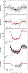 |
Fig. 1 Photometric light curves for NGTS-26. (a) Phase-folded light curve of NGTS-26 discovered with NGTS. The different colours correspond to individual transits. Dark points correspond to a binning of 22.3 min. (b) Phase-folded light curve of TESS, Sector 38 data, without dilution correction. The binning and colours are the same as for a. (c) EulerCam NGTS band, (d) SAAO I band, and (e) SAAO V band. The UT night of each observation is indicated on the plots c–e. |
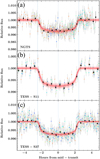 |
Fig. 2 Photometric light curves for NGTS-27. (a) Phase-folded NGTS discovery light curve, (b) Phase-folded TESS, Sector 11 data (with 30-min cadence), (c) Phase-folded TESS, Sector 37 data (with 10-min cadence). For each plot the different colours correspond to individual transits. Dark points correspond to a binning of 29.3 min. |
2.2.2 SAAO
NGTS-26 and NGTS-27 were both observed twice with the Sutherland High-speed Optical Camera (SHOC; Coppejans et al. 2013) instrument on the 1-m telescope at the South African Astronomical Observatory (SAAO). NGTS-26 was first observed on the night beginning 22 April 2018 using an I filter, 20 s exposures and no defocus. The second observation was on 27 March 2019 with a V filter, 60 s exposures and no defocus. NGTS-27 was observed on 5 February 2019 and 27 April 2019. Both observations used an I filter and no defocus. The first observation used 30 s exposures, while the second used 20 s exposures. Calibration frames for the data reduction were taken at sunset and sunrise for bias correcting and flat-fielding. To achieve a high precision, we combined the calibration frames with frames from the remaining observing run and performed bias correction and flat-fielding of the data. We used a background correction for the science frames, and differential aperture photometry was performed using a 5.1-pixel aperture and three fainter comparison stars that are visible in the 2.85′ × 2.85′ field of view. The comparison stars and aperture radius were chosen to maximise the signal-to-noise ratio of the light curve. All photometry was derived using the SEP python package (Barbary 2016), which is based on the core algorithms of the Source Extractor (Bertin & Arnouts 1996). The light curve was detrended with a matern exponential GP kernel using the target position, background, airmass and FWHM. The modelled transits of NGTS-26 and NGTS-27 after GP detrending, are shown in Figs. 1d,e and 3b, respectively.
Summary of the discovery and ground-based follow-up observations of NGTS-26 and NGTS-27.
Sample of additional photometric data of NGTS-26 and NGTS-27 from EulerCam, SAAO, and TESS.
2.2.3 TESS
NGTS-26 (TIC392747437) was observed by the TESS mission (Ricker et al. 2015) in Sector 11, but it lies directly outside the illuminated part of the field of view. Thus, no TESS data were available. The target was re-observed by TESS in April and May 2021 in Sector 38 with Camera 1, CCD 4. Observations were released in July 2021. NGTS-27 (TIC305739565) was observed by TESS in Sector 11 with Camera 1, CCD 1 during April and May 2019 and in Sector 37 with Camera 1, CCD 2 in April 2021. It was identified as TOI-3218 in June 2021 from the faint-star QLP search (Kunimoto et al. 2022). Using the Python astroquery module (Ginsburg et al. 2019) and the according MAST TESS-cut interface (Brasseur et al. 2019), we downloaded cutouts of the area around our targets from the full frame images (FFI) or all available TESS observations. Figure 4 shows the TESS FFIs created using tpfplotter (Aller et al. 2020) centred on NGTS-26 and NGTS-27 in Sectors 38 and 37, respectively. For each sector, photometry extraction was performed independently. Based on the median of all frames, we calculated a master frame that we used to determine the optimal pixel mask for the photometric aperture as well as for the background. With this aperture, we calculated the observed brightness of the star over time and corrected it by the background. Frames with a non-zero quality flag were directly rejected. For NGTS-26, the field is relatively crowded, introducing a significant photometric dilution from neighbouring stars. This dilution factor was adjusted in the global modelling (see Sect. 4). For NGTS-26 five transit events were covered by TESS in Sector 38. For NGTS-27 five and six transit events were covered by TESS in Sector 11 and 37, respectively. The phase-folded TESS light curves of NGTS-26 and NGTS-27 are displayed in Figs. 1b and 2b,c, respectively. As predicted in Wheatley et al. (2018), for such stars with I magnitudes fainter than 12.5, TESS, and NGTS display a similar photometric precision.
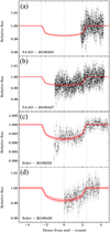 |
Fig. 3 Photometric follow-up light curves for NGTS-27. (a, b) SAAO I band, (c) EulerCam V band, (d) EulerCam B band. The UT night of each observation is indicated on the plots. |
2.3 High resolution spectroscopy
In order to confirm the planetary nature of the two transiting candidates and to measure their masses, we acquired multi-epoch spectroscopy for RV measurements from three different fibre-fed echelle spectrographs, all of which are located at the La Silla Observatory in Chile. A summary of the observations is set out in Table 2. Radial velocity measurements along with activity indicator measurements (i.e. FWHM, bisector span and Hα) are listed in Table 4 and RVs are displayed in Fig. 5.
2.3.1 CORALIE
NGTS-27 was observed with the CORALIE spectrograph on the Swiss 1.2-m telescope at La Silla, Chile (Queloz et al. 2001) between 19 and 24 March 2019. A total of four spectra were obtained. Given the relatively faint magnitude of the star (V = 13.5), we used these spectra for vetting purposes before observing with larger telescopes. Data were reduced using an adapted version of the HARPS standard data reduction pipeline. For each epoch, we derived the RV of the star using the cross-correlation technique (Pepe et al. 2002) using a G2 mask. The observations showed no significant RV variation within the errors of ~60 m s−1 as well as no evidence of a secondary component in the spectra. We thus ruled out SB2 as well as short-period companion with a mass greater than 3 MJup at 3σ.
2.3.2 FEROS
NGTS-26 and NGTS-27 were observed with the FEROS spectrograph on the MPG/ESO 2.2-m telescope at La Silla, Chile (Kaufer et al. 1999). NGTS-26 was observed and vetted under programme 0103-A-9004 with a total of three RVs obtained in June 2019. NGTS-27 was observed under the same programme between 18 April and 9 June 2019, obtaining a total of nine RVs. The data were reduced using the CERES pipeline (Brahm et al. 2017), which in addition to reducing the spectra also calculates RVs by cross-correlating the spectra with a binary G2 mask and fitting a double Gaussian to the cross-correlation function to account for moonlight contamination.
2.3.3 HARPS
We observed both NGTS-26 and NGTS-27 with the HARPS instrument on the 3.6-m ESO telescope, at La Silla (Mayor et al. 2003) under programmes 099.C-0303, 0103.C-0719 and 0104.C-0588 (PI: Bouchy). The observations were conducted between August 2017 and February 2020. For both stars we used the high efficiency mode (EGGS) which utilises a larger fibre than the standard high accuracy mode (HAM). The EGGS-science fibre has a 1.4-arcsec on-sky projection, which results in lower spectral resolution for the final spectrum. This mode is useful for faint stars that are expected to be photon limited in HAM mode. During exposures, we had a second fibre on sky to monitor the background flux. For NGTS-26 we used this measurement to correct for moon contamination in the science spectrum obtained on 9 August 2017. We used the standard HARPS data reduction software (DRS) to derive the radial velocities of the host stars at each epoch by cross-correlating with a binary G2 mask. We also computed the bisector span, FWHM, and activity indicators for each spectrum. We found no evidence for a correlation between the RV and the bisector spans, excluding many blended eclipsing binary scenarios. The observations of NGTS-26 had exposure times ranging between 1800 and 3600 s, resulting in final RV uncertainties of 11–31 m s−1. For NGTS-27 we used an exposure time of 1800 s for which we obtained error bars of 7–14 m s−1.
3 Stellar properties
The extracted HARPS spectra were co-added onto a common wavelength frame to produce a single combined spectrum with an S/N of 40 and 30 for NGTS-26 and NGTS-27 respectively. We analysed these spectra using the spectral analysis package ISPEC (Blanco-Cuaresma et al. 2014). We used the synthesis method to fit individual spectral lines of the co-added spectra. The radiative transfer code SPECTRUM (Gray & Corbally 1994) was used to generate model spectra with MARCS model atmospheres (Gustafsson et al. 2008), version 5 of the GES (Gaia ESO survey) atomic line list provided within ISPEC and solar abundances from Asplund et al. (2009). Macroturbulence was estimated using equation 5.10 from Doyle (2015) and microtur-bulence was accounted for at the synthesis stage using equation 3.1 from the same source. The Hα, Na I D, and Mg I b lines were used to inform Teff and log 𝑔, while Fe I and Fe II lines were used to determine [Fe/H] and υ sin i. Model spectra were synthesised until an acceptable match to the data was found, and uncertainties were estimated by varying individual parameters until model spectra were no longer well matched to the spectra of NGTS-26 and NGTS-27.
To model the SED, we used ARIADNE, a Python tool for fitting stellar SED to broad-band photometry (Vines & Jenkins 2022). In the following, we brielfy summarise the process: We convolved model grids of Phoenix v2 (Husser et al. 2013), BT-Settl, BT-Cond, and BT-NextGen (Hauschildt et al. 1999; Allard et al. 2012; Castelli & Kurucz 2003; Kurucz 1993) with all available filter responses to create six model grids that were then used to fit for the star’s SED. ARIADNE fits for Teff, log 𝑔, [Fe/H], radius, distance, and extinction in the V band, AV, using the spectroscopic parameters as priors for the temperature, gravity, and [Fe/H]; the Gaia DR3 parallax (Gaia Collaboration 2023) as the prior for the distance; and a flat prior for the extinction, limited to the maximum in the line of sight as per the SFD galaxy dust map (Schlegel et al. 1998; Schlafly & Finkbeiner 2011). The posterior space was sampled using dynesty’s nested sampling algorithm (Speagle 2020), which estimates the Bayesian evidence of each model. Finally, the posterior samples of the six models were averaged using each model’s Bayesian evidence as weights in order to get the final posterior distribution for each parameter. The stellar parameters derived for NGTS-26 and NGTS-27 are listed in Tables 5 and 6, respectively.
We also checked the Gaia DR3 astrometric parameters of both targets to exclude evidence of a blended stellar companion or background stars. Proper motions derived from Gaia DR2 and DR3 do not present any significant changes. The two targets do not present any astrometric excess noise. The Gaia re-normalised unit weight error (RUWE) values, which are expected to be close to one for well-behaved single-star solutions and higher than 1.4 for multiple stars, are 1.043 and 0.994 for NGTS-26 and NGTS-27 respectively. The probability from DSC-Combmod of being a single star is higher than 0.9997 in both cases.
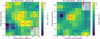 |
Fig. 4 TESS imagettes of 11 × 11 pixels showing the NGTS-26 (left) and NGTS-27 (right) with white cross symbols. Stars in the imagettes, as reported from Gaia DR3, are plotted as red circles. The underlying pixel flux counts in electrons is represented by the blue to yellow colour gradient. Imagettes are taken from Sector 38 (right) and Sector 37 (left). |
4 Global modeling
We jointly modelled the light curves and radial velocities of NGTS-26 and NGTS-27 using GP-EBOP (Gillen et al. 2017, 2020; Smith et al. 2021b) to determine the fundamental and orbital parameters of NGTS-26 b and NGTS-27 b. We note that GP-EBOP comprises a central transiting planet and eclipsing binary model, which utilises Gaussian processes (GP) to account for the effects of stellar activity and other noise signals (e.g. instrumental, weather), and explores the posterior parameter space via Markov chain Monte Carlo (MCMC). Limb darkening coefficients are derived via the analytic method of Mandel & Agol (2002) for the quadratic law and parameterised using the triangular sampling method of Kipping (2013).
The data sets for NGTS-26 and NGTS-27 are reported in Tables 2 and 3. For NGTS-26, we modelled the NGTS discovery light curve, the TESS light curve, three follow-up transit light curves (two SAAO and one Euler), and 17 RVs from HARPS and FEROS. For NGTS-27, we modelled the NGTS discovery light curve, the two TESS light curves, four follow-up transit light curves (two SAAO and two Euler), and 18 RVs from HARPS, FEROS and CORALIE. While neither system shows evidence of stellar variability in the form of detectable rotation signals or flares, low-level activity may still be present and variations will arise from instrumental (both software and hardware) and atmospheric effects. We therefore modelled each light curve with a GP and transit model simultaneously to account for these effects and propagate uncertainties arising from them into the posterior distributions of our planet parameters of interest. We opted to use a Matern-3/2 kernel, as implemented through the Celerite2 package (Foreman-Mackey et al. 2017; Foreman-Mackey 2018), which is well suited to such reasonably rough noise profiles.
With sparse RV coverage, we opted not to include a GP noise component as part of our RV model, and we instead incorporated a white noise jitter term that was added in quadrature to the observed uncertainties. Initial RV orbit values were taken from minimisation estimations performed using The Data & Analysis Center for Exoplanets3 (DACE, see e.g. Delisle et al. 2016), with the initial offsets between instruments, δγ, set to zero, which were then allowed to vary in subsequent test runs on the full data sets.
Within GP-EBOP, the stellar and planetary parameters fit are the radius ratio (RP/R*), radius sum ((R* + RP) /a), cosine of the inclination (cos i), orbital period (P), time of central transit (TC), systemic velocity (Vsys), RV semi-amplitude (K*), white noise jitter terms for each instrument (e.g. σharps), and an RV offset from HARPS for the FEROS and CORALIE RVs (e.g. δeros). Wide uniform priors were used for all of these parameters.
The limb darkening profiles, and hence parameters, were constrained using the predictions of the Limb Darkening Toolkit (LDTK – Parviainen & Aigrain 2015) based on the Teff, log g, and [Fe/H] values reported in Tables 5 and 6. Uncertainties were inflated by a factor of 10 to account for systematic uncertainties in stellar atmosphere models at the Teff, log 𝑔, and [Fe/H] of NGTS-26 and NGTS-27. For NGTS-26, the TESS photometry contains significant dilution from neighbour stars, so we opted to allow a free floating dilution term (of the form contamination flux/total flux) with a wide uniform prior when fitting the TESS data. We found a dilution factor 0.437 ± 0.044. No significant dilution was predicted or detected in the TESS data of NGTS-27. The NGTS light curves were binned to a 5-min cadence with the GP-EBOP model binned accordingly. All other data sets were modelled at the cadence reported in Table 2.
To explore the posterior parameter space, we used 250 ‘walkers’ and 200 000 steps, with the first 100 000 steps discarded as a conservative burn-in and the remaining steps thinned by a factor of 500. The posterior values (16th, 50th, and 84th percentiles) for the fundamental and orbital planet parameters of NGTS-26 b and NGTS-27 b are reported in Tables 7 and 8, respectively.
We found that NGTS-26 b has a mass and radius of  and
and  and orbits its host star in P = 4.5199279 ± 0.0000091 days at an orbital distance of
  AU. Similarly, we found that NGTS-27 b has a mass and radius of
  and
and  and orbits its host star in P = 3.3704181 ± 0.0000058 days at an orbital distance of
  .
.
Radial velocity observations along with activity indicator measurements FWHM, bisector, Hα of NGTS-26, and NGTS-27 from HARPS, FEROS, and CORALIE.
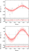 |
Fig. 5 Radial velocities of NGTS-26 and NGTS-27. Top: phase-folded radial velocities of NGTS-26. Circles and triangles correspond to HARPS and FEROS measurements respectively. The lower plot shows the data with the model removed. Bottom: phase-folded radial velocities of NGTS-27. Circles, triangles, and diamonds correspond to HARPS, FEROS and CORALIE measurements, respectively. The lower plot shows the data with the model removed. |
5 Discussion and conclusions
NGTS-26 b and NGTS-27 b are shown in Fig. 6 on the mass-radius diagram with other known transiting exoplanets. Both NGTS-26 b and NGTS-27 b are highly irradiated by their host stars with an incident flux above the threshold of 2 × 10⁵ W m−2 (or 147 times the Earth insolation) corresponding to the lower limit where gas giants are increasingly found with anomalously larger radii than theoretically predicted (Guillot & Showman 2002; Miller & Fortney 2011; Demory & Seager 2011). Using the stellar luminosity from Gaia DR2 and the orbital parameters, we computed the irradiation level received by NGTS-26 b and NGTS-27 b to be a factor 3.5 and 11 times larger than this limit, respectively.
Assuming the models from Baraffe et al. (2008) with typical hot Jupiter irradiation (Sun at 0.045 AU), an age of 7 Gyr, and a heavy element mass fraction of Z = 0.02, NGTS-26 b and NGTS-27b would have theoretical radii close to 1.06–1.07 RJup. Assuming the models from Fortney et al. (2007) with an equivalent temperature of 1960 K and 1300 K, an age of 4.5 Gyr, and a massless core, NGTS-26 b and NGTS-27 b would have theoretical radii of 1.05 RJup and 1.19 RJup, respectively. Therefore, the two new NGTS giant planets, with radii of  and 1.40 ± 0.04 RJup, have anomalously inflated radii. Knowing that NGTS-26 is slightly metal rich with [Fe/H]=0.2±0.1 dex, and that the Sun’s heavy element mass fraction is close to 2%, we may suspect that the heavy element enrichment could be larger than 2%, which would make the inflated radius even more anomalous. Considering the age of these two systems, the mechanisms causing inflated planet radii need to be able to operate late in the evolution of a planetary system.
Following Sestovic et al. (2018), who established an empirical relationship between the radii of planets and their incident stellar flux for four different mass ranges, we estimated the predicted radius inflation parameter ∆R. This excess radius ∆R is dependent on the incident flux and the planet mass, and it is derived with respect to a ‘baseline’ radius of 0.98 ± 0.04 RJup. We found  and
and  for NGTS-26 b and NGTS-27 b respectively. With an observed radius of
  , NGTS-26 b is definitively unexpectedly inflated. NGTS-26 b is one of the largest objects amongst peers of similar mass. As seen in Fig. 6, it lies well above similar objects. With such a low density, we may suspect that NGTS-26 b has a negligible core mass. NGTS-26 b is, however, relatively similar to highly inflated Saturn-mass objects with masses in the range of 0.2−0.4 MJup and radii larger than 1.3 RJup, such as WASP-153 b (Demangeon et al. 2018), WASP-63 b (Hellier et al. 2012; Bonomo et al. 2017), WASP-20 b (Anderson et al. 2015), WASP-39b (Faedi et al. 2011), and HAT-P-58 b (Bakos et al. 2021), with an expected very low fraction of heavy elements.
Sestovic et al. (2018) claimed that below 0.37 MJup giant exoplanets are unable to maintain inflated radii larger than 1.4 RJup and instead exhibit smaller sizes as the incident flux is increased beyond 106 W m−2. Our result for NGTS-26 b, as with the other published highly inflated Saturn-mass objects, does not seem to validate this claim. We suspect that the Sestovic et al. (2018) result comes from the very low number of Saturn-mass planets with strong irradiation used in their study (mainly based on three exoplanets). Discovery and characterisation of highly irradiated Saturn-mass exoplanets similar to NGTS-26 b will be helpful in revisiting this relationship.
We note that radial velocities of NGTS-26 b are quite noisy and sparse, which is reflected in its mass uncertainty. Our RV noise model is a simple white noise jitter term added in quadrature to the observed uncertainties. Due to the small number of RVs, we cannot completely exclude that the mass uncertainty of NGTS-26 b is slightly underestimated, and hence it could take the planet towards the inner edge of the more massive planet population.
With an observed radius of 1.40 ± 0.04 RJup, NGTS-27 b presents a radius similar to other hot Jupiters of the same mass and irradiation level (see Fig. 6). The expected radius excess  is even slightly larger (2-σ) than the observed radius, meaning that NGTS-27 b is somewhat less inflated than expected, and we may suspect that this hot Jupiter possesses a significant massive core. We also note that its host star is likely evolving off the main sequence and the observed planetary radius could also be linked to the evolution of the irradiated hot Jupiter, as postulated by Lopez & Fortney (2016). This type of possible trend between stellar evolution and reinfliation of planets was also recently reported by several studies of individual systems, such as HD 221416 (Huber et al. 2019), HD 1397 (Brahm et al. 2019), and NGTS-13 (Grieves et al. 2021).
Different mechanisms have been proposed to explain the anomalously large radii of hot Jupiters, including ohmic dissipation (Batygin & Stevenson 2010), advection of potential temperature (Tremblin et al. 2017), and thermal tides (Arras & Socrates 2010). Thorngren & Fortney (2018) showed that the heating efficiency increases as a function of equilibrium temperature, with a shape providing evidence for ohmic dissipation. They discussed the fact that below about 0.4 MJup, considerably fewer highly irradiated planets are detected, an effect not seen in low-irradiated planets. It is possible that significant mass loss could occur if planets undergo very significant inflation, and that could explain the lack of highly inflated low-mass planets. An alternative hypothesis is that Saturn-mass planets preferentially stop migration further from the parent star.
Assuming zero albedo, efficient heat redistribution and the measured mass, we computed the equilibrium temperature of NGTS-26 b and NGTS-27 b to be  and
and  , respectively, and the scale height to be 1200 ± 300 km and 940 ± 140 km, respectively. The addition of one scale height to each planet’s radius, as might be induced by a chemical species with strong wavelength-dependent absorption, would cause the transit depth difference for NGTS-26 b and NGTS-27 b to be 380 ± 80 ppm and 130 ± 20 ppm, respectively. These relatively small differences combined with the faint magnitude of host stars make detailed atmospheric characterisation of these two planets very challenging with current instruments.
Stellar parameters for NGTS-26.
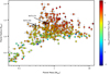 |
Fig. 6 Mass-radius diagram of known exoplanets from the PlanetS catalogue (https://dace.unige.ch/exoplanets/), April 2023, based on reliable, robust, and as much accurate mass (better than 25%) and radius (better than 8%) measurements of transiting planets as possible. The colour of the symbols indicates the incident flux from the host star in Earth units. The locations of NGTS-26 b and NGTS-27 b are shown with black outlined symbols. |
Stellar parameters for NGTS-27.
Planetary properties for NGTS-26 b.
Planetary properties for NGTS-27 b.
Acknowledgements
This study is based on observations collected at the European Southern Observatory under ESO programmes 099.C-0303, 0103.C-0719, 0104.C-0588 and 0103.A-9004. We thank the Swiss National Science Foundation (SNSF) and the Geneva University for their continuous support to our planet search programmes. This work has been in particular carried out in the frame of the National Centre for Competence in Research PlanetS supported by the SNSF. This publication makes use of The Data & Analysis Center for Exoplanets (DACE), which is a facility based at the University of Geneva dedicated to extrasolar planets data visualisation, exchange and analysis. This paper includes data collected by the TESS mission. Funding for the TESS mission is provided by the NASA Explorer Program. This paper uses observations made at the South African Astronomical Observatory (SAAO). E.G. gratefully acknowledges support from the David and Claudia Harding Foundation in the form of a Winton Exoplanet Fellowship, and from the UK Science and Technology Facilities Council (STFC; project reference ST/W001047/1). J.S.J. gratefully acknowledges support by FONDECYT grant 1201371 and from the ANID BASAL projects ACE210002 and FB210003. This research was funded in part by the UKRI (Grants ST/X001121/1, EP/X027562/1). M.N.G. acknowledges support from the European Space Agency (ESA) as an ESA Research Fellow. M.L. acknowledges support of the Swiss National Science Foundation under grant number PCEFP2_194576. C.A.W. would like to acknowledge support from the STFC (grant number ST/X00094X/1). This work made use of tpfplotter by J. Lillo-Box (publicly available in www.github.com/jlillo/tpfplotter), which also made use of the python packages astropy, lightkurve, matplotlib and numpy. The Digitized Sky Surveys were produced at the Space Telescope Science Institute under U.S. Government grant NAG W-2166. The images of these surveys are based on photographic data obtained using the Oschin Schmidt Telescope on Palomar Mountain and the UK Schmidt Telescope. The plates were processed into the present compressed digital form with the permission of these institutions.
References
- Allard, F., Homeier, D., & Freytag, B. 2012, Philos. Trans. Roy. Soc. A: Math.Phys. Eng. Sci., 370, 2765 [NASA ADS] [CrossRef] [Google Scholar]
- Aller, A., Lillo-Box, J., Jones, D., Miranda, L. F., & Barcelo Forteza, S. 2020, A&A, 635, A128 [NASA ADS] [CrossRef] [EDP Sciences] [Google Scholar]
- Anderson, D. R., Collier Cameron, A., Hellier, C., et al. 2015, A&A, 575, A61 [NASA ADS] [CrossRef] [EDP Sciences] [Google Scholar]
- Armstrong, D. J., Gunther, M. N., McCormac, J., et al. 2018, MNRAS, 478, 4225 [NASA ADS] [CrossRef] [Google Scholar]
- Arras, P., & Socrates, A. 2010, ApJ, 714, 1 [Google Scholar]
- Asplund, M., Grevesse, N., Sauval, A. J., & Scott, P. 2009, ARA&A, 47, 481 [NASA ADS] [CrossRef] [Google Scholar]
- Bakos, G. Á., Hartman, J. D., Bhatti, W., et al. 2021, AJ, 162, 7 [NASA ADS] [CrossRef] [Google Scholar]
- Baraffe, I., Chabrier, G., & Barman, T. 2008, A&A, 482, 315 [NASA ADS] [CrossRef] [EDP Sciences] [Google Scholar]
- Barbary, K. 2016, J. Open Source Softw., 1, 58 [Google Scholar]
- Batygin, K., & Stevenson, D. J. 2010, ApJ, 714, L238 [NASA ADS] [CrossRef] [Google Scholar]
- Bayliss, D., Gillen, E., Eigmiiller, P., et al. 2018, MNRAS, 475, 4467 [NASA ADS] [CrossRef] [Google Scholar]
- Bayliss, D., Wheatley, P., West, R., et al. 2020, The Messenger, 181, 28 [NASA ADS] [Google Scholar]
- Bertin, E., & Arnouts, S. 1996, A&AS, 117, 393 [NASA ADS] [CrossRef] [EDP Sciences] [Google Scholar]
- Blanco-Cuaresma, S., Soubiran, C., Heiter, U., & Jofré, P. 2014, A&A, 569, A111 [CrossRef] [EDP Sciences] [Google Scholar]
- Bonomo, A. S., Desidera, S., Benatti, S., et al. 2017, A&A, 602, A107 [NASA ADS] [CrossRef] [EDP Sciences] [Google Scholar]
- Brahm, R., Jordán, A., & Espinoza, N. 2017, PASP, 129, 034002 [Google Scholar]
- Brahm, R., Espinoza, N., Jordán, A., et al. 2019, AJ, 158, 45 [Google Scholar]
- Brasseur, C. E., Phillip, C., Fleming, S. W., Mullally, S. E., & White, R. L. 2019, Astrocut: Tools for creating cutouts of TESS images Astrophysics Source Code Library [record ascl:1905.007] [Google Scholar]
- Castelli, F., & Kurucz, R. L. 2003, in Modelling of Stellar Atmospheres, eds. N. Piskunov, W. W. Weiss, & D. F. Gray, IAU Symposium, 210, A20 [NASA ADS] [Google Scholar]
- Chaushev, A., Raynard, L., Goad, M. R., et al. 2019, MNRAS, 488, 5232 [Google Scholar]
- Collier Cameron, A., Pollacco, D., Street, R. A., et al. 2006, MNRAS, 373, 799 [Google Scholar]
- Coppejans, R., Gulbis, A. A. S., Kotze, M. M., et al. 2013, PASP, 125, 976 [Google Scholar]
- Dawson, R. I., & Johnson, J. A. 2018, ARA&A, 56, 175 [Google Scholar]
- Delisle, J. B., Ségransan, D., Buchschacher, N., & Alesina, F. 2016, A&A, 590, A134 [NASA ADS] [CrossRef] [EDP Sciences] [Google Scholar]
- Demangeon, O. D. S., Faedi, F., Hébrard, G., et al. 2018, A&A, 610, A63 [NASA ADS] [CrossRef] [EDP Sciences] [Google Scholar]
- Demory, B.-O., & Seager, S. 2011, ApJS, 197, 12 [NASA ADS] [CrossRef] [Google Scholar]
- Doyle, A. P. 2015, PhD thesis, Keele University [Google Scholar]
- Faedi, F., Barros, S. C. C., Anderson, D. R., et al. 2011, A&A, 531, A40 [NASA ADS] [CrossRef] [EDP Sciences] [Google Scholar]
- Foreman-Mackey, D. 2018, RNAAS, 2, 31 [NASA ADS] [Google Scholar]
- Foreman-Mackey, D., Agol, E., Ambikasaran, S., & Angus, R. 2017, AJ, 154, 220 [Google Scholar]
- Fortney, J. J., Marley, M. S., & Barnes, J. W. 2007, ApJ, 659, 1661 [Google Scholar]
- Fortney, J. J., Dawson, R. I., & Komacek, T. D. 2021, J. Geophys. Res. (Planets), 126, e06629 [NASA ADS] [Google Scholar]
- Gaia Collaboration (Vallenari, A., et al.) 2023, A&A, 674, A1 [NASA ADS] [CrossRef] [EDP Sciences] [Google Scholar]
- Gill, S., Wheatley, P. J., Cooke, B. F., et al. 2020, ApJ, 898, L11 [Google Scholar]
- Gillen, E., Hillenbrand, L. A., David, T. J., et al. 2017, ApJ, 849, 11 [Google Scholar]
- Gillen, E., Hillenbrand, L. A., Stauffer, J., et al. 2020, MNRAS, 495, 1531 [CrossRef] [Google Scholar]
- Ginsburg, A., Sipocz, B. M., Brasseur, C. E., et al. 2019, AJ, 157, 98 [NASA ADS] [CrossRef] [Google Scholar]
- Gray, R. O., & Corbally, C. J. 1994, AJ, 107, 742 [Google Scholar]
- Grieves, N., Nielsen, L. D., Vines, J. I., et al. 2021, A&A, 647, A180 [NASA ADS] [CrossRef] [EDP Sciences] [Google Scholar]
- Guillot, T., & Showman, A. P. 2002, A&A, 385, 156 [NASA ADS] [CrossRef] [EDP Sciences] [Google Scholar]
- Gustafsson, B., Edvardsson, B., Eriksson, K., et al. 2008, A&A, 486, 951 [NASA ADS] [CrossRef] [EDP Sciences] [Google Scholar]
- Hauschildt, P. H., Allard, F., & Baron, E. 1999, ApJ, 629, 865 [Google Scholar]
- Hellier, C., Anderson, D. R., Collier Cameron, A., et al. 2012, MNRAS, 426, 739 [NASA ADS] [CrossRef] [Google Scholar]
- Hou, Q., & Wei, X. 2022, MNRAS, 511, 3133 [NASA ADS] [CrossRef] [Google Scholar]
- Huber, D., Chaplin, W. J., Chontos, A., et al. 2019, AJ, 157, 245 [Google Scholar]
- Husser, T.-O., Wende-von Berg, S., Dreizler, S., et al. 2013, A&A, 553, A6 [NASA ADS] [CrossRef] [EDP Sciences] [Google Scholar]
- Jackson, B., Miller, N., Barnes, R., et al. 2010, MNRAS, 407, 910 [NASA ADS] [CrossRef] [Google Scholar]
- Kaufer, A., Stahl, O., Tubbesing, S., et al. 1999, The Messenger, 95, 8 [Google Scholar]
- Kipping, D. M. 2013, MNRAS, 435, 2152 [Google Scholar]
- Kovács, G., Zucker, S., & Mazeh, T. 2002, A&A, 391, 369 [Google Scholar]
- Kunimoto, M., Daylan, T., Guerrero, N., et al. 2022, ApJS, 259, 33 [NASA ADS] [CrossRef] [Google Scholar]
- Kurucz, R. 1993, ATLAS9 Stellar Atmosphere Programs and 2 km/s grid, Kurucz CD-ROM No. 13 (Cambridge), 13 [Google Scholar]
- Lendl, M., Anderson, D. R., Collier-Cameron, A., et al. 2012, A&A, 544, A72 [NASA ADS] [CrossRef] [EDP Sciences] [Google Scholar]
- Lopez, E. D., & Fortney, J. J. 2016, ApJ, 818, 4 [NASA ADS] [CrossRef] [Google Scholar]
- Mandel, K., & Agol, E. 2002, ApJ, 580, L171 [Google Scholar]
- Mayor, M., Pepe, F., Queloz, D., et al. 2003, The Messenger, 114, 20 [NASA ADS] [Google Scholar]
- Mazeh, T., Holczer, T., & Faigler, S. 2016, A&A, 589, A75 [NASA ADS] [CrossRef] [EDP Sciences] [Google Scholar]
- McCormac, J., Gillen, E., Jackman, J. A. G., et al. 2020, MNRAS, 493, 126 [Google Scholar]
- Miller, N., & Fortney, J. J. 2011, ApJ, 736, L29 [NASA ADS] [CrossRef] [Google Scholar]
- Parviainen, H., & Aigrain, S. 2015, MNRAS, 453, 3821 [Google Scholar]
- Pepe, F., Mayor, M., Rupprecht, G., et al. 2002, The Messenger, 110, 9 [NASA ADS] [Google Scholar]
- Petigura, E. A., Marcy, G. W., Winn, J. N., et al. 2018, AJ, 155, 89 [Google Scholar]
- Queloz, D., Mayor, M., Udry, S., et al. 2001, The Messenger, 105, 1 [NASA ADS] [Google Scholar]
- Ricker, G. R., Winn, J. N., Vanderspek, R., et al. 2015, J. Astron. Telescopes Instrum. Syst., 1, 014003 [Google Scholar]
- Schlafly, E. F., & Finkbeiner, D. P. 2011, ApJ, 737 [Google Scholar]
- Schlegel, D. J., Finkbeiner, D. P., & Marc, D. 1998, ApJ, 525 [Google Scholar]
- Sestovic, M., Demory, B.-O., & Queloz, D. 2018, A&A, 616, A76 [NASA ADS] [CrossRef] [EDP Sciences] [Google Scholar]
- Smith, A. M. S., Acton, J. S., Anderson, D. R., et al. 2021a, A&A, 646, A183 [NASA ADS] [CrossRef] [EDP Sciences] [Google Scholar]
- Smith, G. D., Gillen, E., Queloz, D., et al. 2021b, MNRAS, 507, 5991 [CrossRef] [Google Scholar]
- Speagle, J. S. 2020, MNRAS, 493, 3132 [Google Scholar]
- Spiegel, D. S., & Burrows, A. 2013, ApJ, 772, 76 [Google Scholar]
- Tamuz, O., Mazeh, T., & Zucker, S. 2005, MNRAS, 356, 1466 [Google Scholar]
- Thorngren, D. P., & Fortney, J. J. 2018, AJ, 155, 214 [Google Scholar]
- Thorngren, D. P., Lee, E. J., & Lopez, E. D. 2023, ApJ, 945, L36 [NASA ADS] [CrossRef] [Google Scholar]
- Tremblin, P., Chabrier, G., Mayne, N. J., et al. 2017, ApJ, 841, 30 [NASA ADS] [CrossRef] [Google Scholar]
- Vines, J. I., & Jenkins, J. S. 2022, MNRAS, 513, 2719 [NASA ADS] [CrossRef] [Google Scholar]
- Vines, J. I., Jenkins, J. S., Acton, J. S., et al. 2019, MNRAS, 489, 4125 [NASA ADS] [CrossRef] [Google Scholar]
- West, R. G., Gillen, E., Bayliss, D., et al. 2019, MNRAS, 486, 5094 [Google Scholar]
- Wheatley, P. J., West, R. G., Goad, M. R., et al. 2018, MNRAS, 475, 4476 [Google Scholar]
All Tables
Summary of the discovery and ground-based follow-up observations of NGTS-26 and NGTS-27.
Sample of additional photometric data of NGTS-26 and NGTS-27 from EulerCam, SAAO, and TESS.
Radial velocity observations along with activity indicator measurements FWHM, bisector, Hα of NGTS-26, and NGTS-27 from HARPS, FEROS, and CORALIE.
All Figures
|
Fig. 1 Photometric light curves for NGTS-26. (a) Phase-folded light curve of NGTS-26 discovered with NGTS. The different colours correspond to individual transits. Dark points correspond to a binning of 22.3 min. (b) Phase-folded light curve of TESS, Sector 38 data, without dilution correction. The binning and colours are the same as for a. (c) EulerCam NGTS band, (d) SAAO I band, and (e) SAAO V band. The UT night of each observation is indicated on the plots c–e. |
| In the text | |
|
Fig. 2 Photometric light curves for NGTS-27. (a) Phase-folded NGTS discovery light curve, (b) Phase-folded TESS, Sector 11 data (with 30-min cadence), (c) Phase-folded TESS, Sector 37 data (with 10-min cadence). For each plot the different colours correspond to individual transits. Dark points correspond to a binning of 29.3 min. |
| In the text | |
|
Fig. 3 Photometric follow-up light curves for NGTS-27. (a, b) SAAO I band, (c) EulerCam V band, (d) EulerCam B band. The UT night of each observation is indicated on the plots. |
| In the text | |
|
Fig. 4 TESS imagettes of 11 × 11 pixels showing the NGTS-26 (left) and NGTS-27 (right) with white cross symbols. Stars in the imagettes, as reported from Gaia DR3, are plotted as red circles. The underlying pixel flux counts in electrons is represented by the blue to yellow colour gradient. Imagettes are taken from Sector 38 (right) and Sector 37 (left). |
| In the text | |
|
Fig. 5 Radial velocities of NGTS-26 and NGTS-27. Top: phase-folded radial velocities of NGTS-26. Circles and triangles correspond to HARPS and FEROS measurements respectively. The lower plot shows the data with the model removed. Bottom: phase-folded radial velocities of NGTS-27. Circles, triangles, and diamonds correspond to HARPS, FEROS and CORALIE measurements, respectively. The lower plot shows the data with the model removed. |
| In the text | |
|
Fig. 6 Mass-radius diagram of known exoplanets from the PlanetS catalogue (https://dace.unige.ch/exoplanets/), April 2023, based on reliable, robust, and as much accurate mass (better than 25%) and radius (better than 8%) measurements of transiting planets as possible. The colour of the symbols indicates the incident flux from the host star in Earth units. The locations of NGTS-26 b and NGTS-27 b are shown with black outlined symbols. |
| In the text | |
Current usage metrics show cumulative count of Article Views (full-text article views including HTML views, PDF and ePub downloads, according to the available data) and Abstracts Views on Vision4Press platform.
Data correspond to usage on the plateform after 2015. The current usage metrics is available 48-96 hours after online publication and is updated daily on week days.
Initial download of the metrics may take a while.