| Issue |
A&A
Volume 656, December 2021
Solar Orbiter First Results (Cruise Phase)
|
|
|---|---|---|
| Article Number | L10 | |
| Number of page(s) | 8 | |
| Section | Letters to the Editor | |
| DOI | https://doi.org/10.1051/0004-6361/202140966 | |
| Published online | 14 December 2021 | |
Letter to the Editor
Evidence for local particle acceleration in the first recurrent galactic cosmic ray depression observed by Solar Orbiter
The ion event on 19 June 2020⋆
1
Dept. de Física Quàntica i Astrofísica, Institut de Ciències del Cosmos (ICCUB), University de Barcelona (UB-IEEC), Barcelona, Spain
e-mail: angels.aran@fqa.ub.edu
2
Institute of Experimental and Applied Physics, Kiel University, 24118 Kiel, Germany
3
INAF/Istituto di Astrofisica e Planetologia Spaziali, Via del Fosso del Cavaliere 100, 00133 Roma, Italy
4
Centre for mathematical Plasma-Astrophysics, Dept. of Mathematics, KU Leuven, Celestijnenlaan 200B, 3001 Leuven, Belgium
5
Heliophysics Science Division, NASA Goddard Space Flight Center, Greenbelt, MD 20771, USA
6
Dept. of Astronomy, University of Maryland, Maryland, MD 20742, USA
7
Solar-Terrestrial Centre of Excellence – SIDC, Royal Observatory of Belgium, 1180 Brussels, Belgium
8
Now at Paradox Cat GmbH, 80333 Mnchen, Germany
9
George Mason University, Fairfax, VA 22030, USA
10
Universidad de Alcalá, Space Research Group, 28805 Alcalá de Henares, Spain
11
Swedish Institute of Space Physics (IRF), Uppsala, Sweden
12
Space Plasma Physics, Department of Physics and Astronomy, Uppsala University, Uppsala 75120, Sweden
13
LESIA, Observatoire de Paris, Université PSL, CNRS, Sorbonne Université, Université de Paris, 5 place Jules Janssen, 92195 Meudon, France
14
Radboud Radio Lab, Dept. of Astrophysics, Radboud University, Nijmegen, The Netherlands
15
Goddard Planetary Heliophysics Institute, University of Maryland, Baltimore County, Baltimore, MD, USA
16
Institute of Physics, University of Maria Curie-Skłodowska, ul. Radziszewskiego 10, 20-031 Lublin, Poland
17
Johns Hopkins University Applied Physics Laboratory, Laurel, MD, USA
18
Dept. of Physics, Imperial College London, London SW7 2AZ, UK
19
Now at DSI Datensicherheit GmbH, Rodendamm 34, 28816 Stuhr, Germany
20
Institut de Recherche en Astrophysique et Planétologie, 9 avenue du Colonel Roche, BP 4346, 31028 Toulouse Cedex 4, France
21
European Space Agency (ESA), European Space Astronomy Centre (ESAC), Villanueva de la Cañada, Madrid, Spain
22
Now at Deutsches Elektronen-Synchrotron (DESY), Platanenallee 6, 15738 Zeuthen, Germany
23
National Observatory of Athens, Institute for Astronomy, Astrophysics, Space Applications and Remote Sensing, Athens, Greece
24
Now at German Aerospace Center (DLR), Dept. of Extrasolar Planets and Atmospheres, Berlin, Germany
25
Dept. of Space and Climate Physics, University College London, Holmbury St Mary, Dorking RH5 6NT, UK
26
Now at Max-Planck-Institute for Solar System Research, Justus-von-Liebig-Weg 3, 37077 Göttingen, Germany
27
Now at University of Colorado/LASP, Boulder, CO, USA
28
Skobeltsyn Institute of Nuclear Physics, Moscow State University, Moscow, Russia
Received:
31
March
2021
Accepted:
1
August
2021
Context. In mid-June 2020, the Solar Orbiter (SolO) mission reached its first perihelion at 0.51 au and started its cruise phase, with most of the in situ instruments operating continuously.
Aims. We present the in situ particle measurements of the first proton event observed after the first perihelion obtained by the Energetic Particle Detector (EPD) suite on board SolO. The potential solar and interplanetary (IP) sources of these particles are investigated.
Methods. Ion observations from ∼20 keV to ∼1 MeV are combined with available solar wind data from the Radio and Plasma Waves (RPW) instrument and magnetic field data from the magnetometer on board SolO to evaluate the energetic particle transport conditions and infer the possible acceleration mechanisms through which particles gain energy. We compare > 17–20 MeV ion count rate measurements for two solar rotations, along with the solar wind plasma data available from the Solar Wind Analyser (SWA) and RPW instruments, in order to infer the origin of the observed galactic cosmic ray (GCR) depressions.
Results. The lack of an observed electron event and of velocity dispersion at various low-energy ion channels and the observed IP structure indicate a local IP source for the low-energy particles. From the analysis of the anisotropy of particle intensities, we conclude that the low-energy ions were most likely accelerated via a local second-order Fermi process. The observed GCR decrease on 19 June, together with the 51.8–1034.0 keV nuc−1 ion enhancement, was due to a solar wind stream interaction region (SIR). The observation of a similar GCR decrease in the next solar rotation favours this interpretation and constitutes the first observation of a recurrent GCR decrease by SolO. The analysis of the recurrence times of this SIR suggests that it is the same SIR responsible for the 4He events previously measured in April and May. Finally, we point out that an IP structure more complex than a common SIR cannot be discarded, mainly due to the lack of solar wind temperature measurements and the lack of a higher cadence of solar wind velocity observations.
Key words: acceleration of particles / Sun: heliosphere / solar wind
Movies associated to Figs. B.1 and B.2 are available at https://www.aanda.org
© ESO 2021
1. Introduction
Shortly after Solar Orbiter (SolO; Müller et al. 2020) was launched, on 10 February 2020 (UT time), the sensors of the Energetic Particle Detector (EPD; Rodríguez-Pacheco et al. 2020) on board SolO started performing regular measurements of electrons, protons, and heavy ions. Wimmer-Schweingruber et al. (2021) summarise the first year of EPD operations, providing information on the data products supplied by the different EPD sensors and listing the first near-relativistic electron and ion intensity enhancements measured by EPD. Mason et al. (2021) report on the first 3He-rich solar energetic particle (SEP) events observed by SolO. Allen et al. (2021) list the first 4He enhancements associated with stream interaction regions (SIRs) observed both by SolO and the Advanced Composition Explorer (ACE) spacecraft (SC), including the first recurrent ion event, in April–May 2020. The first large SEP event ever detected by SolO occurred on 29 November 2020 (Kollhoff et al. 2021).
In addition to SolO, Parker Solar Probe (PSP) also provides measurements of low-energy ions in the inner heliosphere associated with SIRs (e.g., Allen et al. 2020a; Cohen et al. 2020; Desai et al. 2020). These measurements, in combination with solar wind plasma and interplanetary magnetic field (IMF) data, are key to understanding the various particle acceleration mechanisms acting in interplanetary (IP) space. For example, Wijsen et al. (2021) model the transport and acceleration undergone by the particles responsible for an SIR low-energy proton event on 19 September 2019, observed by both PSP and the Solar Terrestrial Relations Observatory Ahead (STEREO-A) SC, and conclude that the particles were accelerated at the compression waves associated with the observed SIR. On the other hand, Richardson (1985) and Schwadron et al. (1996, 2020) analysed other SIR events, showing that second-order Fermi acceleration processes contribute to local ion acceleration in SIRs.
The effects that solar wind perturbations produce on the intensity of galactic cosmic rays (GCRs) at a given heliospheric location make GCR measurements an excellent probe of the passage of IP structures. For example, interplanetary coronal mass ejections (ICMEs) may cause GCR intensity depressions known as Forbush decreases (FDs; Forbush 1937), whose morphological aspects at different locations are related to the spatial and temporal evolution of the ICMEs. For the classical two-step FD (Barnden 1973), the maximum FD amplitude is reached in two phases, associated first with the shock or the sheath of the ICME and then with the main body of the ICME or ejecta (see Richardson & Cane 2011, and references therein). The passage of corotating high-speed solar wind streams (HSSs) may also produce GCR depressions (e.g., Iucci et al. 1979; Richardson 2004, 2018, and references therein), also called recurrent FDs by some authors. In general, GCR decreases are produced by the strong or turbulent magnetic field structures associated with ICMEs and SIRs (resulting from the interaction of HSSs with the slow solar wind) that may act as barriers in the GCR transport. Closed magnetic fields in ICMEs and increased convection in HSSs are also other mechanisms that modulate the GCR intensities. A description of the different physical mechanisms involved can be found in Cane (2000) for ICMEs and in Richardson (2018) for HSSs. Several FDs have been observed in space by the most recent missions (e.g., Armano et al. 2018; Benella et al. 2020, and references therein), including the ICME-induced FD on 19 April 2020 recorded by SolO/EPD (Freiherr von Forstner et al. 2021).
In this paper we analyse low-energy ion and GCR measurements by SolO during the period 18–20 June 2020 when the SC was at ∼0.52 au from the Sun. Using solar wind data and magnetic field data provided by various instruments on board SolO, we determine the particle sources and discuss the plausible particle acceleration processes producing the observed low-energy event. We identify, for the first time, the observations of a recurrent FD at SolO. In Sect. 2 we describe the various particle data products used and the magnetic field measurements. In Sect. 3 we analyse the GCR measurements provided by the High Energy Telescope (HET) of EPD (Rodríguez-Pacheco et al. 2020). In Sect. 4 we discuss the possible particle sources of the low-energy particles, and conclusions are reported in Sect. 5.
2. The observed ion event
Figure 1 summarises the particle and magnetic field measurements from SolO during the period 18–20 June 2020. In particular, in the top two panels we show the ion differential intensity enhancements measured by the SupraThermal Electrons and Protons (STEP) sensor, the Electron-Proton Telescope (EPT), and HET (Rodríguez-Pacheco et al. 2020). The corresponding ion measurements from the Suprathermal Ion Spectrograph (SIS) were analysed by Mason et al. (2021). During this period, SolO moved from 0.517 au to 0.521 au in heliocentric radial distance, and from 257.9° to 266.3° in longitude and from 6.7° to 6.6° in latitude in Heliocentric Inertial (HCI) coordinates.
 |
Fig. 1. Summary of suprathermal-to-energetic proton measurements by EPD and IMF measurements from MAG. Top panel: differential intensities for four energy channels from STEP (18.6–47.8 keV nuc−1) and eight channels (51.8–1034.0 keV nuc−1) from the EPT Sun telescope. Second panel: > 17–20 MeV nuc−1 ion count rates from the HET1 and HET2 telescopes. Third panel: IMF intensity. Bottom panel: radial (grey), tangential (orange), and normal (blue) components in the SC-centred RTN coordinate system. It should be noted that the IMF configuration departs from a nominal Archimedean spiral, as indicated by the Bn and Bt excursions. |
The top panel of Fig. 1 shows: [1] 5-min averages of ion differential intensities measured in four energy channels between 18.6 keV nuc−1 and 47.8 keV nuc−1 as constructed from the STEP ‘rates’ data product; [2] 5-min averages of the ion differential intensity measured by the EPT Sun telescope in eight energy channels (51.8–1034.0 keV nuc−1) and constructed from the ‘hcad’ (high-cadence) data product of EPT. The magnet channels of both sensors detect ions that are mostly protons, except for background intensity levels or events with soft energy spectrum, where the contribution of He ions can be large (Wimmer-Schweingruber et al. 2021). Hereafter, keeping this in mind, we refer to these particles as ions or protons indistinctly. The second panel of Fig. 1 shows > 17–20 MeV nuc−1 ion count rates measured by the HET Sun-Antisun (HET1; blue line) and the North-South (HET2; orange line) telescopes. These single-detector count rates correspond to GCR particles detected by the HET C detector, which is detailed in Freiherr von Forstner et al. (2021). There were no particle intensity enhancements measured by the differential channels of the HET telescopes. Finally, the bottom panel of Fig. 1 displays 1-min averages of the intensity (black line) and radial-tangential-normal (RTN) components (colour-code as indicated) of the IMF measurements from the magnetometer (MAG) on board SolO (Horbury et al. 2020). These data are available at the Solar Orbiter Archive (SOAR)1.
The low-energy (< 40 keV) ion intensities start to increase above background levels after 04:00 UT on 18 June. This increase coincides with a decrease in the high-energy ion count rates (second panel of Fig. 1). The pitch angles of the < 40 keV ions (not shown here) indicate that these particles propagated mostly away from the Sun. The shape of the ion differential intensity-time profiles evolves gradually across energies. Intensities start to increase at later times with increasing energy, so that for the EPT lowest energy channel, the intensity increases only on day 19 at 00:45 UT simultaneously with a sudden enhancement observed up to ∼124 keV. This latter enhancement coincides with a second (smaller) decrease in the high-energy count rates detected by HET and an increased IMF intensity. Two hours later, there is a simultaneous peak observed in all the EPT channels displayed. The peak values of the 44.0–47.8 keV nuc−1 channel of STEP and of the 51.8–67.5 keV channel of EPT are very similar due to the different aperture width of the two telescopes (Rodríguez-Pacheco et al. 2020) and due to their different detection efficiency (e.g., Wimmer-Schweingruber et al. 2021). The peak is followed by a rapid decrease and another more gradual increase in the intensities (∼08:00 UT on 19 June).
Figure 2 shows the EPT 5-min-averaged ion intensities for the same energy channels as in Fig. 1 but for the four telescopes of EPT: the Sun, the Anti-Sun (Asun), the North, and the South telescopes, as indicated in the top four panels of Fig. 2. The mean energy of the channels and the corresponding colours are indicated in the second panel. As can be seen, the Asun telescope only detects a tiny gradual ion intensity enhancement at the lower energy channels, after 08:00 UT on 19 June, in coincidence with the other three fields of view (FoVs). The North and South telescopes also detect a simultaneous increase in intensities between 02:00–04:45 UT on 19 June in the energy range 59–517 keV. The bottom panel of Fig. 2 shows the evolution of the pitch angles of the particles entering each of the telescopes. The changes in the pitch angle of each FoV reflect the magnetic structures observed during this period as well as the reversals of the magnetic field polarity (see Appendix A). The strong Sun-Asun anisotropy observed in the particle intensities and the pitch angles covered by the Sun telescope suggest that the particles mostly flow away from the Sun.
 |
Fig. 2. Low-energy ion intensities (energy channels indicated in the legend) observed by EPT in each FoV: Sunward (top panel), anti-sunward (second panel), North (third panel), and South (fourth panel). Bottom panel: the pitch angles observed by each FoV (colour-code indicated in the legend). |
There were no electron intensity enhancements observed by EPT nor STEP in the period 18–22 June, and no radio-wave bursts were detected by SolO. Only a weak Type III radio burst was detected by STEREO-A, PSP, and the Wind SC on 18 June between 13:00 and 13:30 UT (not shown here). However, the lack of an electron event and the fact that these three SC were separated by more than 58°, eastward from SolO, suggest that there was no direct magnetic connection between the solar source site of the radio burst and SolO. Only narrow and slow coronal mass ejections (CMEs) were observed during the five days before this particle event. In the next sections, we discuss the origin of the GCR depressions observed on 18 and 19 June by analysing the available solar wind plasma and IMF data, and we further analyse the directional intensities detected by the EPT telescopes and the modulation of the particle intensities due to the IMF structures detected.
3. Analysis of the galactic cosmic ray decreases
The high-energy ion count rates detected by the HET telescope (middle panel in Fig. 1) are a measure of the GCR background. The top panel of Fig. 3 shows the GCR intensity for the period 17–24 June (black line), obtained by adding the > 17–20 MeV ion count rates from all the HET counters in order to achieve high counting statistics, following the method described by Freiherr von Forstner et al. (2021). These count rates were normalised to a reference value, defined by the average count rate over the quiet-time period from 00:00 UT on 5 June to 00:00 UT on 8 June 2020. The time profile (black line) shows an event characterised by an initial short-term GCR intensity increase and two consecutive decreases of different amplitudes.
 |
Fig. 3. GCR depressions. From top to bottom: time profile of HET normalised ion count rates, solar wind speed, density, and magnetic field magnitude for the period from 09:36 UT on 16 June to 09:35 UT on 24 June (black lines) and from 00:00 UT on 19 July to 00:00 UT on 27 July (green lines). The time difference between the two periods is 32.6 days. The black vertical line indicates the start of the second GCR depression at 22:00 UT on 18 June. |
The first decrease starts at ∼00:00 UT on 18 June and reaches the minimum intensity at 11:00 UT with an hourly percentage variation of about 4%, whereas the second decrease starts at 22:00 UT on 18 June (solid vertical line) and has a variation of about 2%, reaching the minimum value at 18:00 UT on 19 June. Such a behaviour suggests a two-step FD related to the transit of a shock or ICME, or to the passage of two different IP structures, one of which is a corotating interaction region (CIR) between a slow wind and an HSS, as discussed below.
Solar wind plasma measurements of the Solar Wind Analyser (SWA) instrument on board SolO (Owen et al. 2020) were not available for the studied period in June. Instead, we used the solar wind plasma electron density and velocity values derived from measurements of the Radio Plasma Waves (RPW) instrument on board SolO (Maksimovic et al. 2020) in order to identify the driver of the observed GCR decreases. The solar wind density was obtained from the probe-to-SC potential (VPSP; for more details, see Khotyaintsev et al. 2021). The radial solar wind speed was derived by using the method detailed in Steinvall et al. (2021) and averaging the velocities over 6-h intervals to reduce noise. We point out that such solar wind speed data can only be considered as a rough estimate over large timescales to distinguish between fast and slow solar wind (Steinvall et al. 2021). The RPW solar wind speed and density for the period 16–24 June are shown in the second and third panels of Fig. 3 (black lines), respectively. The black line in the bottom panel shows the IMF intensity as measured by MAG during the same time interval. A low solar wind speed, an irregular and filamentary density profile with moderate values, and a high IMF intensity can be observed concomitantly with the beginning of the first GCR decrease. A new magnetic field increase starting at 22:00 UT on 18 June, accompanied by an increase in the solar wind speed and a later decrease in the solar wind density (until ∼08:00 UT 19 June), suggests that an HSS, possible corotating, swept over SolO. The start of the second decrease at 22:00 UT on 18 June is close to the CIR stream interface around midnight.
We looked for a possible recurrence of the suggested HSS structure by considering plasma, particle, and IMF data during the next solar rotation. We combined the solar rotation and the SolO motion (in the direction of the solar rotation) to compute the time delay for the second encounter at SolO of the same IP magnetic structure. We found that the recurrent structure observed at ∼22:00 UT on June 18 would have reached SolO on the next solar rotation in 32.6 days, that is, at ∼11:30 UT on 21 July, when SolO was at 0.68 au. We over-plot in Fig. 3 the normalised GCR intensity, the plasma parameters recorded by SWA, and the MAG magnetic field data for 32.6 days later (top X axis, green lines). A GCR decrease is observed to begin at ∼12:00 UT on 21 July, in very good agreement with the estimated recurrence time. In addition, the shape of the intensity-time profile (green line in the top panel of Fig. 3) and its minimum value (∼2% at 16:00 UT) match the 19 June decrease (black line), suggesting their association with the same IP structure. Moreover, a stream interface is observed on 21 July ahead of an HSS, thus supporting the interpretation that a CIR crossed SolO on 19 June. The recurrence of the same CIR in previous solar rotations is computed to be on 20 May and 23 April, which almost coincide with the time of corotating suprathermal ion events identified by Allen et al. (2021) as CIR1 and CIR3 (see their Table 1 and Fig. 4).
By contrast, the corresponding 18 June decrease is not observed and the IMF intensity-time profiles are different on 18 June and 21 July. This suggests three possible causes for the first GCR decrease at 00:00 on 18 June: [1] a transient structure, also responsible for the short-term GCR increase before the decrease; [2] the interval from 18 to 19 June is more complicated than a normal CIR, possibly including encounters with the heliospheric plasma sheet (which give rise to periods where the density is enhanced and the field is relatively depressed); and [3] the solar source of the HSS changed its shape, especially its latitudinal extent (see Wimmer-Schweingruber et al. 1997, 1999, for an in-depth discussion).
4. Analysis of the low-energy ion event
The top panel of Fig. 4 shows the proton intensity-time profiles observed by the EPT Sun telescope after applying the Compton-Getting correction detailed in Appendix A. The energy values indicated in the legend correspond to the mean energies of the differential intensity channels. The second panel shows the values of the pitch-angle cosine (red line), μ, in the solar wind frame, corresponding to 68 keV protons, together with the μ values for protons of similar energies detected by the other telescopes. The estimated Sun-Asun anisotropy, A∥, for ∼68 keV protons (see Appendix A) is displayed in the third panel of Fig. 4, in the SC (black line) and solar wind (blue line) reference frames. The remaining panels of Fig. 4 show (up to down) the solar wind speed and density from RPW and the IMF intensity, elevation, and azimuthal angles from MAG.
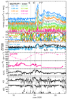 |
Fig. 4. Summary of particle and IP data from SolO during the period 18–20 June 2020. From top to bottom: (1) 51–786 keV proton differential intensities obtained from the EPT Sun telescope and conveniently transformed into the solar wind reference frame; (2) pitch-angle cosine of the different FoVs of the EPT sensor in the solar wind reference frame for 68 keV protons. Grey dots at 1.0 and −1.0 indicate the positive and negative polarity of the IMF following Eq. (1) in Pacheco et al. (2019); (3) the ∼68 keV proton Sun-Asun anisotropy A∥; (4) estimation of the solar wind speed as derived from RPW measurements; (5) solar wind density as provided by RPW; and (6) IMF intensity, (7) elevation, and (8) azimuthal angles in RTN coordinates as provided by MAG. The different solar wind regimes in the CIR are identified (S, S′, F′, and F regions) and separated by vertical lines. |
Prior to the particle intensity enhancement at ∼00:45 UT on 19 June, ∼68 keV proton intensities were at background levels. The similar background intensities in both the Sun and Asun telescopes (cf. Fig. 2) result in A∥ ∼ 0 in the SC reference frame but A∥ < 0 in the solar wind reference frame. Since no particle intensity enhancement was observed during this period, negative values of A∥ do not imply that an actual sunward flow of CIR-associated particles was observed. By contrast, the intensity increase early on 19 June clearly showed an anti-sunward flow of ∼68 keV protons. This intensity increase coincides with the arrival of the HSS, together with a complex profile of the solar wind density and the second increase in the compressed magnetic field.
The shape of the intensity profiles and the IP conditions on 19 June shown in Fig. 4 resemble those of the low-energy ion event on 21–26 June 1979 associated with a CIR reported by Richardson & Zwickl (1984). Following the work of these authors, we have divided the CIR into four regions: the slow solar wind (S), the accelerated slow solar wind (S′), the compressed and decelerated fast solar wind (F′), and the unperturbed fast solar wind (F). The vertical lines in Fig. 4 indicate the boundaries between these regions. We note that the stream interface location (between S′ and F′) is approximated due to the lack of plasma temperature measurements and the rough temporal cadence of the solar wind speed. The EPT instrumental background intensities prevent us from assessing the flow direction of the particles in the S region, which in the case of the event analysed by Richardson & Zwickl (1984) was a sunward flow. However, similar to what Richardson & Zwickl (1984) observed in the 1979 event, actual sunward anisotropies are observed in the late F region, and a clear anti-sunward flow is detected in the F′ region. From the analysis of particle anisotropies, intensity energy spectra, and a complete set of solar wind variables, Richardson & Zwickl (1984) and Richardson (1985) suggested that the low-energy ions during the event on 21–26 June 1979 were accelerated locally via a stochastic (second-order Fermi) process. In our event, [1] the above coincidence of the anisotropy sign in the F′ and F regions, [2] the rather weak compressed solar wind in the CIR, and [3] simultaneous increase and peak of the intensities in the different channels in F′ seem to rule out the acceleration of these particles by a distant region of the CIR and make a local stochastic acceleration process a plausible mechanism to explain the observed sudden low-energy ion enhancement.
Signatures such as the anti-sunward flow of particles early in the F region and the apparent flow direction of the ions measured by STEP (see Sect. 2) are more difficult to explain. Hence, we can envision a more complex IP scenario than depicted above, such as: [1] the occurrence of multiple stream interfaces within the CIR (e.g., Wimmer-Schweingruber et al. 1997); or [2] the small CME eruption observed by the SolO Extreme Ultraviolet Imager (EUI) instrument (Rochus et al. 2020) on 17 June (see Appendix B) arrived at the end of 18 June and compressed the CIR. In the latter case, in addition to the local acceleration in the CIR, the acceleration of particles by the CME-related disturbance could explain the abovementioned signatures; particles injected from a distant source may exhibit anti-sunward anisotropies inside the CIR, depending on the energy of the particles (Wijsen et al. 2019).
5. Conclusions
We have studied the ion event that took place on 18–20 June 2020 by combining multiple datasets provided by the in situ instruments of SolO. We show that a recurrent SIR crossed SolO on 19 June, producing an anisotropic < 1 MeV ion intensity enhancement and a decrease in the GCR intensity. This is the first evidence of a CIR crossing SolO as identified by using in situ solar wind parameters as well as the first recurrent GCR depressions, of about 2% amplitude on 19 June and 21 July, in addition to magnetic field data and ion enhancements. Moreover, the computation of the recurrence times in previous solar rotations suggests that this CIR can be associated with the corotating suprathermal ion enhancements on 19 May and 23 April found by Allen et al. (2021).
From the analysis of energetic particle anisotropies, the identification of the CIR from the observed recurrent GCR depression, and the similarities with previously analysed CIR particle events, we conclude that the low-energy ion intensity enhancement observed on 19 June 2020 at SolO was most likely produced by a local stochastic acceleration process. The variety of particle measurements provided by SolO are key for studying the location of the particle acceleration sites. The 18–20 June 2020 event illustrates that even small particle events are difficult to interpret, such that the combination of in situ and remote-sensing observations is needed, and SolO is equipped for such a challenge.
Movies
Movie 1 associated with Fig. B.1. Access here
Movie 2 associated with Fig. B.2. Access here
Acknowledgments
Solar Orbiter is a mission of international collaboration between ESA and NASA, operated by ESA. EPD was built with funding from Ministerio de Ciencia e Innovación (Spain), Deutsches Zentrum für Luft- und Raumfahrt (Germany), and the European Space Agency (ESA); operations are funded by FEDER/MCI/AEI Projects ESP2017-88436-R and PID2019-104863RBI00/AEI/10.13039/501100011033 (Spain), 50OT 2002 (DLR, Germany), and NASA contract 80MSFC19F0002. The UB team acknowledges the support by the Spanish Ministerio de Ciencia e Innovación (MICINN) under grant PID2019-105510GB-C31 and through the “Center of Excellence María de Maeztu 2020-2023” award to the ICCUB (CEX2019-000918-M). The CAU Kiel team acknowledges support by the German Federal Ministry for Economic Affairs and Energy, the German Space Agency (Deutsches Zentrum für Luft- und Raumfahrt e.V., DLR) under grants 50OT0901, 50OT1202, 50OT1702, 50OT2002, and 50OC1702. The Solar Orbiter magnetometer was funded by the UK Space Agency (grant ST/T001062/1). M.L. and S.B. acknowledge financial support by the Italian MIUR-PRIN grant 2017APKP7T on Circumterrestrial Environment: Impact of Sun-Earth Interaction. N.W. acknowledges funding from the Research Foundation – Flanders (FWO – Vlaanderen, fellowship no. 1184319N). D.L. acknowledges the support from the NASA-HGI grant NNX16AF73G and the NASA Programs NNH17ZDA001N-LWS. I.G.R. and D.L. acknowledge support from NASA program NNH19ZDA001N-LWS. E.S. was supported by a PhD grant awarded by the Royal Observatory of Belgium. V.K. acknowledges the support by NASA under grants 18-2HSWO218_2-0010 and 19-HSR-19_2-0143. S.P. is supported by the projects C14/19/089 (C1 project Internal Funds KU Leuven), G.0D07.19N (FWO-Vlaanderen), SIDEX (ESA Prodex-12), and EUHFORIA 2.0 (funding from the European Union’s Horizon 2020 research and innovation programme under grant agreement No 870405). IRFU team acknowledges support from the Swedish National Space Agency grant 20/136. F.C. acknowledges the financial support by the Spanish MINECO-FPI-2016 predoctoral grant with FSE. The JHU/APL team is supported under NASA contract NNN06AA01C and thanks NASA headquarters and the NASA/GSFC Solar Orbiter project office for their continuing support. Solar Orbiter Solar Wind Analyser (SWA) data are derived from scientific sensors which have been designed and created, and are operated under funding provided in numerous contracts from the UK Space Agency (UKSA, most recently grant ST/T001356/1), the UK Science and Technology Facilities Council (STFC), the Agenzia Spaziale Italiana (ASI), the Centre National d’Etudes Spatiales (CNES, France), the Centre National de la Recherche Scientifique (CNRS, France), the Czech contribution to the ESA PRODEX programme and NASA. The RPW instrument has been designed and funded by CNES, CNRS, the Paris Observatory, The Swedish National Space Agency, ESA-PRODEX and all the participating institutes. The authors thank the Belgian Federal Science Policy Office (BELSPO) for the provision of financial support in the framework of the PRODEX Programme of the European Space Agency (ESA) under contract number 4000112292. The EUI instrument was built by CSL, IAS, MPS, MSSL/UCL, PMOD/WRC, ROB, LCF/IO with funding from the Belgian Federal Science Policy Office (BELPSO); the Centre National d’Etudes Spatiales (CNES); the UK Space Agency (UKSA); the Bundesministerium für Wirtschaft und Energie (BMWi) through the Deutsches Zentrum für Luft und Raumfahrt (DLR); and the Swiss Space Office (SSO). SWAP is a project of the Centre Spatial de Liége and the Royal Observatory of Belgium funded by the Belgian Federal Science Policy Office (BELSPO). EUI and SWAP images were processed using JHelioviewer, (Müller et al. 2017), JHelioviewer is part of the ESA/NASA Helioviewer Project.
References
- Allen, R. C., Lario, D., Odstrcil, D., et al. 2020a, ApJS, 246, 36 [Google Scholar]
- Allen, R. C., Mason, G. M., Ho, G. C., et al. 2021, A&A, 656, L2 (SO Cruise Phase SI) [NASA ADS] [CrossRef] [EDP Sciences] [Google Scholar]
- Armano, M., Audley, H., Baird, J., et al. 2018, ApJ, 854, 113 [NASA ADS] [CrossRef] [Google Scholar]
- Barnden, L. 1973, Int. Cosmic R. Conf., 2, 1277 [NASA ADS] [Google Scholar]
- Benella, S., Laurenza, M., Vainio, R., et al. 2020, ApJ, 901, 21 [NASA ADS] [CrossRef] [Google Scholar]
- Brueckner, G. E., Howard, R. A., Koomen, M. J., et al. 1995, Sol. Phys., 162, 357 [NASA ADS] [CrossRef] [Google Scholar]
- Cane, H. V. 2000, Space Sci. Rev., 93, 55 [NASA ADS] [CrossRef] [Google Scholar]
- Cohen, C. M. S., Christian, E. R., Cummings, A. C., et al. 2020, ApJS, 246, 20 [Google Scholar]
- Compton, A. H., & Getting, I. A. 1935, Phys. Rev., 47, 817 [NASA ADS] [CrossRef] [Google Scholar]
- Desai, M. I., Mitchell, D. G., Szalay, J. R., et al. 2020, ApJS, 246, 56 [Google Scholar]
- Forbush, S. E. 1937, Phys. Rev., 51, 1108 [NASA ADS] [CrossRef] [Google Scholar]
- Forman, M. A. 1970, Planet. Space Sci., 18, 25 [Google Scholar]
- Freiherr von Forstner, J. L., Dumbović, M., Möstl, C., et al. 2021, A&A, 656, A1 (SO Cruise Phase SI) [NASA ADS] [CrossRef] [EDP Sciences] [Google Scholar]
- Halain, J. P., Berghmans, D., Seaton, D. B., et al. 2013, Sol. Phys., 286, 67 [NASA ADS] [CrossRef] [Google Scholar]
- Horbury, T. S., O’Brien, H., Carrasco Blazquez, I., et al. 2020, A&A, 642, A9 [NASA ADS] [CrossRef] [EDP Sciences] [Google Scholar]
- Ipavich, F. M. 1974, Geophys. Res. L, 1, 149 [NASA ADS] [CrossRef] [Google Scholar]
- Iucci, N., Parisi, M., Storini, M., & Villoresi, G. 1979, Il Nuovo Cimento C, 2, 421 [CrossRef] [Google Scholar]
- Khotyaintsev, Yu. V., Graham, D., Vaivads, A., et al. 2021, A&A, 656, A19 (SO Cruise Phase SI) [NASA ADS] [CrossRef] [EDP Sciences] [Google Scholar]
- Kilpua, E. K. J., Good, S. W., Dresing, N., et al. 2021, A&A, 656, A8 (SO Cruise Phase SI) [NASA ADS] [CrossRef] [EDP Sciences] [Google Scholar]
- Kollhoff, A., Kouloumvakos, A., Lario, D., et al. 2021, A&A, 656, A20 (SO Cruise Phase SI) [NASA ADS] [CrossRef] [EDP Sciences] [Google Scholar]
- Maksimovic, M., Bale, S. D., Chust, T., et al. 2020, A&A, 642, A12 [EDP Sciences] [Google Scholar]
- Mason, G. M., Ho, G. C., Allen, R. C., et al. 2021, A&A, 656, L1 (SO Cruise Phase SI) [NASA ADS] [CrossRef] [EDP Sciences] [Google Scholar]
- Müller, D., Nicula, B., Felix, S., et al. 2017, A&A, 606, A10 [Google Scholar]
- Müller, D., St. Cyr, O. C., Zouganelis, I., et al. 2020, A&A, 642, A1 [Google Scholar]
- Owen, C. J., Bruno, R., Livi, S., et al. 2020, A&A, 642, A16 [EDP Sciences] [Google Scholar]
- Pacheco, D., Agueda, N., Aran, A., Heber, B., & Lario, D. 2019, A&A, 624, A3 [NASA ADS] [CrossRef] [EDP Sciences] [Google Scholar]
- Richardson, I. G. 1985, Planet. Space Sci., 33, 557 [NASA ADS] [CrossRef] [Google Scholar]
- Richardson, I. G. 2004, Space Sci. Rev., 111, 267 [Google Scholar]
- Richardson, I. G. 2018, Liv. Rev. Sol. Phys., 15, 1 [Google Scholar]
- Richardson, I. G., & Cane, H. V. 2011, Sol. Phys., 270, 609 [NASA ADS] [CrossRef] [Google Scholar]
- Richardson, I. G., & Zwickl, R. D. 1984, Planet. Space Sci., 32, 1179 [NASA ADS] [CrossRef] [Google Scholar]
- Rochus, P., Auchère, F., Berghmans, D., et al. 2020, A&A, 642, A8 [NASA ADS] [CrossRef] [EDP Sciences] [Google Scholar]
- Rodríguez-Pacheco, J., Wimmer-Schweingruber, R. F., Mason, G. M., et al. 2020, A&A, 642, A7 [Google Scholar]
- Schwadron, N. A., Fisk, L. A., & Gloeckler, G. 1996, Geophys. Res. L, 23, 2871 [NASA ADS] [CrossRef] [Google Scholar]
- Schwadron, N. A., Joyce, C. J., Aly, A., et al. 2020, A&A, 650, A24 [Google Scholar]
- Seaton, D. B., Berghmans, D., Nicula, B., et al. 2013, Sol. Phys., 286, 43 [NASA ADS] [CrossRef] [Google Scholar]
- Steinvall, K., Khotyaintsev, Yu. V., Cozzani, G., et al. 2021, A&A, 656, A9 (SO Cruise Phase SI) [NASA ADS] [CrossRef] [EDP Sciences] [Google Scholar]
- Wijsen, N., Aran, A., Pomoell, J., & Poedts, S. 2019, A&A, 624, A47 [NASA ADS] [CrossRef] [EDP Sciences] [Google Scholar]
- Wijsen, N., Samara, E., Aran, A., et al. 2021, ApJ, 908, L26 [CrossRef] [Google Scholar]
- Wimmer-Schweingruber, R. F., von Steiger, R., & Paerli, R. 1997, J. Geophys. Res., 102, 17407 [NASA ADS] [CrossRef] [Google Scholar]
- Wimmer-Schweingruber, R. F., von Steiger, R., & Paerli, R. 1999, J. Geophys. Res., 104, 9933 [CrossRef] [Google Scholar]
- Wimmer-Schweingruber, R. F., Janitzek, N. P., Pacheco, D., et al. 2021, A&A, 656, A22 (SO Cruise Phase SI) [NASA ADS] [CrossRef] [EDP Sciences] [Google Scholar]
Appendix A: Ion intensities in the solar wind frame
In the study of the transport of energetic particles it is assumed that turbulent fluctuations are convected with the bulk of the plasma flow. Therefore, in order to analyse the pitch-angle and anisotropy distributions of the particles it is convenient to transform the directional intensities observed in the SC reference frame to a reference frame co-moving with the solar wind because the anisotropy of a particle distribution may change in a different frame of reference. This process is referred to as the Compton-Getting correction (Compton & Getting 1935; Forman 1970; Ipavich 1974). The Compton-Getting effect is significant for low-energy ions (< 2 MeV/nuc).
In the classical limit, the speed, V′, of a particle in the solar wind frame is related to its speed, V, in the SC reference frame by

where U < < c is the solar wind speed and θ is the angle between the solar wind velocity, U, and the particles entering the telescope in its looking direction, V (Ipavich 1974). From this transformation it is easy to show that the pitch angle in the solar wind frame is (e.g., Kilpua et al. 2021)

The distribution function of particles with a given momentum is a Lorentz invariant (Forman 1970). Therefore, in the classical limit the differential intensity of the particles, J′, in the solar wind frame is (e.g., Kilpua et al. 2021)

where μSC and J in the equations above are the particle’s pitch angle and differential intensity, respectively, in the SC frame.
We derived μ and J′ by making the following assumptions: [1] the solar wind velocity derived from RPW is purely radial; [2] we obtained U(t) by linear interpolation between each pair of the 6-hour solar wind speed data to obtain a solar wind speed value every 1 minute, the same cadence of the IMF and of the values of μSC used in these calculations; [3] the particles populating each energy channel have the same kinetic energy, and it is equal to the mean energy of the channel; and [4] ions are protons.
For each FoV of the EPT sensor, Fig. A.1 shows the resulting differential intensities in the solar wind frame corresponding to the eight energy channels of EPT shown in Fig. 2 (top panels) and the 5-minute averages of the pitch-angle cosine, μ, corresponding to the 106.2 keV channel in the SC frame (bottom panels). Given the different looking directions, the Compton-Getting corrections affect the energy spectrum of the particle intensities in each FoV differently. The energy ranges indicated in the legends correspond to the variation in the mean energy of each channel due to the evolution of U and θ during the entire event (18 June to 20 June). The same applies to the values of μ (orange) that now, in the solar wind frame, correspond to protons of different energies in each field of view. In the bottom panels of Fig. A.1, we have plotted μSC (black curves). The Compton-Getting corrections are small and more noticeable for the North and South telescopes due to the lower absolute values of their pitch-angle cosines. For completion, we calculated the IMF polarity sign following Eq. (1) in Pacheco et al. (2019) and plotted it in the μ panels (grey dots). A +1 polarity means that the IMF points away from the Sun, whereas -1 indicates a sunward-pointing IMF. This helps in identifying rapid changes of μ in the Sun-Asun FoV due to IMF polarity reversals.
 |
Fig. A.1. Low-energy ion event as seen in the solar wind reference frame. From top to bottom: EPT Sun, Asun, North, and South telescopes. Top panel: Compton-Getting corrected ion intensities for each energy channel. Bottom panel: μ of the centre of the look direction of the FoV in the SC-centred frame, μSC (black trace), and in the solar wind frame, μ (orange trace). In the latter case, μ corresponds to the third energy channels. Grey dots indicate the polarity of the IMF (1 anti-sunward, -1 sunward). |
As anisotropy information is essential to disentangle the location of the particle’s acceleration sites, we approximated the Sun-Asun anisotropy for protons of ∼68 keV, A∥ as follows:

where the sub-indices sun and asun correspond to the Sun and Asun telescopes, respectively. Since these telescopes point along the nominal IMF configuration, A∥ is a rough approximation to the first-order parallel anisotropy of the particles’ distribution function. The A∥ in the SC reference frame was obtained by using the two lower energy channels of EPT, whereas for A∥ in the solar wind frame we used the values of μ and I for 64 – 73 keV and the 64 – 74 keV protons for the Sun and Asun FoVs (see the two upper panels of Fig. A.1). We note that the mean energy of these protons is ∼68 keV, and hence A∥ is obtained from intensities of particles of the same energy.
Appendix B: A small CME detected by EUI
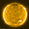 |
Fig. B.1. SolO/EUI image of a small eruption at 08:09 UT on 17 June. The red circle shows the location of the filament. The temporal evolution is available as an online movie. |
At 08:09 UT on 17 June 2020, the Full Sun Imager (FSI) of the SolO/EUI instrument suite (Rochus et al. 2020) detected a filament that started to wiggle in the 174 Å extreme-UV passband2. The location in the solar disk of this filament is indicated by the red circle in Fig. B.1. The associated propagating coronal dimming can be seen by the red circle in the running difference image of Fig. B.2. Movies of both direct and running difference images of the filament eruption are provided in the supplementary material.
Figure B.3 was taken by The Sun Watcher using the Active Pixel System detector and Image Processing (SWAP; Seaton et al. 2013; Halain et al. 2013) telescope on board the PRoject for Onboard Autonomy (PROBA2) mission. The PROBA2 is at a Sun-synchronous orbit around Earth located 66° east of SolO. The PROBA2/SWAP difference image shows a weak eruption off the west limb that was not captured by the Large Angle and Spectrometric Coronagraph Experiment (LASCO; Brueckner et al. 1995) on board the Solar and Heliospheric Observatory (SOHO). Assuming the appearance of the filament to be the earliest time for the small eruption, such a CME would have arrived at SolO, at 22:00 UT on 18 June, in 38 hours. This yields a transit speed of ∼570 km s−1, roughly consistent with the ∼500 km s−1 solar wind speed values provided by SolO/RPW measurements at that time. Nevertheless, the 6-hour cadence of the solar wind speed and the lack of solar wind temperature measurements makes it difficult to confirm whether a disturbance related to this CME arrived at SolO.
 |
Fig. B.2. SolO/EUI running difference image showing the location of the filament and the coronal dimming seen by EUI. The temporal evolution is available as an online movie. |
 |
Fig. B.3. PROBA2/SWAP base difference image of a small CME eruption (marked by the red rectangle) at 10:48 UT on 17 June. |
All Figures
|
Fig. 1. Summary of suprathermal-to-energetic proton measurements by EPD and IMF measurements from MAG. Top panel: differential intensities for four energy channels from STEP (18.6–47.8 keV nuc−1) and eight channels (51.8–1034.0 keV nuc−1) from the EPT Sun telescope. Second panel: > 17–20 MeV nuc−1 ion count rates from the HET1 and HET2 telescopes. Third panel: IMF intensity. Bottom panel: radial (grey), tangential (orange), and normal (blue) components in the SC-centred RTN coordinate system. It should be noted that the IMF configuration departs from a nominal Archimedean spiral, as indicated by the Bn and Bt excursions. |
| In the text | |
|
Fig. 2. Low-energy ion intensities (energy channels indicated in the legend) observed by EPT in each FoV: Sunward (top panel), anti-sunward (second panel), North (third panel), and South (fourth panel). Bottom panel: the pitch angles observed by each FoV (colour-code indicated in the legend). |
| In the text | |
|
Fig. 3. GCR depressions. From top to bottom: time profile of HET normalised ion count rates, solar wind speed, density, and magnetic field magnitude for the period from 09:36 UT on 16 June to 09:35 UT on 24 June (black lines) and from 00:00 UT on 19 July to 00:00 UT on 27 July (green lines). The time difference between the two periods is 32.6 days. The black vertical line indicates the start of the second GCR depression at 22:00 UT on 18 June. |
| In the text | |
|
Fig. 4. Summary of particle and IP data from SolO during the period 18–20 June 2020. From top to bottom: (1) 51–786 keV proton differential intensities obtained from the EPT Sun telescope and conveniently transformed into the solar wind reference frame; (2) pitch-angle cosine of the different FoVs of the EPT sensor in the solar wind reference frame for 68 keV protons. Grey dots at 1.0 and −1.0 indicate the positive and negative polarity of the IMF following Eq. (1) in Pacheco et al. (2019); (3) the ∼68 keV proton Sun-Asun anisotropy A∥; (4) estimation of the solar wind speed as derived from RPW measurements; (5) solar wind density as provided by RPW; and (6) IMF intensity, (7) elevation, and (8) azimuthal angles in RTN coordinates as provided by MAG. The different solar wind regimes in the CIR are identified (S, S′, F′, and F regions) and separated by vertical lines. |
| In the text | |
|
Fig. A.1. Low-energy ion event as seen in the solar wind reference frame. From top to bottom: EPT Sun, Asun, North, and South telescopes. Top panel: Compton-Getting corrected ion intensities for each energy channel. Bottom panel: μ of the centre of the look direction of the FoV in the SC-centred frame, μSC (black trace), and in the solar wind frame, μ (orange trace). In the latter case, μ corresponds to the third energy channels. Grey dots indicate the polarity of the IMF (1 anti-sunward, -1 sunward). |
| In the text | |
|
Fig. B.1. SolO/EUI image of a small eruption at 08:09 UT on 17 June. The red circle shows the location of the filament. The temporal evolution is available as an online movie. |
| In the text | |
|
Fig. B.2. SolO/EUI running difference image showing the location of the filament and the coronal dimming seen by EUI. The temporal evolution is available as an online movie. |
| In the text | |
|
Fig. B.3. PROBA2/SWAP base difference image of a small CME eruption (marked by the red rectangle) at 10:48 UT on 17 June. |
| In the text | |
Current usage metrics show cumulative count of Article Views (full-text article views including HTML views, PDF and ePub downloads, according to the available data) and Abstracts Views on Vision4Press platform.
Data correspond to usage on the plateform after 2015. The current usage metrics is available 48-96 hours after online publication and is updated daily on week days.
Initial download of the metrics may take a while.