| Issue |
A&A
Volume 707, March 2026
|
|
|---|---|---|
| Article Number | A111 | |
| Number of page(s) | 10 | |
| Section | Cosmology (including clusters of galaxies) | |
| DOI | https://doi.org/10.1051/0004-6361/202557038 | |
| Published online | 05 March 2026 | |
The oldest Milky Way stars: New constraints on the age of the Universe and the Hubble constant
1
Dipartimento di Fisica e Astronomia “Augusto Righi”–Università di Bologna Via Piero Gobetti 93/2 I-40129 Bologna, Italy
2
INAF – Osservatorio di Astrofisica e Scienza dello Spazio di Bologna Via Piero Gobetti 93/3 I-40129 Bologna, Italy
3
Leibniz-Institut für Astrophysik Potsdam (AIP) An der Sternwarte 16 14482 Potsdam, Germany
4
Institut für Physik und Astronomie, Universität Potsdam Karl-Liebknecht-Str. 24/25 14476 Potsdam, Germany
5
Departament de Física Quàntica i Astrofísica (FQA), Universitat de Barcelona (UB) Martí i Franquès 1 08028 Barcelona, Spain
6
Institut de Ciències del Cosmos (ICCUB), Universitat de Barcelona (UB) Martí i Franquès 1 08028 Barcelona, Spain
7
Institut d’Estudis Espacials de Catalunya (IEEC), Edifici RDIT, Campus UPC 08860 Castelldefels (Barcelona), Spain
8
Instituto de Astrofísica de Canarias E-38200 La Laguna Tenerife, Spain
9
Departamento de Astrofísica, Universidad de La Laguna E-38205 La Laguna Tenerife, Spain
10
Kavli Institute for Cosmological Physics, University of Chicago 5640 S. Ellis Avenue Chicago IL 60637, USA
★ Corresponding author: This email address is being protected from spambots. You need JavaScript enabled to view it.
Received:
29
August
2025
Accepted:
17
December
2025
Abstract
Aims. In this work, we exploit the most robust, old, and cosmology-independent age estimates of individual stars from Gaia DR3 to place a lower bound on the age of the Universe, tU. These constraints can be used as an anchor point for any cosmological model, thus providing an upper limit to the Hubble constant H0.
Methods. Our primary stellar age catalog comprises 3000 of the oldest and most robustly measured main-sequence turn-off (MSTO) and subgiant branch (SGB) stars, with ages older than 12.5 Gyr and associated uncertainty below 1 Gyr. Stellar ages are derived via isochrone fitting using the Bayesian code StarHorse, spanning the uniform range 0−20 Gyr, not considering any cosmological prior knowledge on tU. By applying a conservative cut in the Kiel diagram and strict quality cuts on both stellar parameters and posterior probability distribution shapes, and filtering out potential contaminants, we isolated a final sample of 160 bona fide stars, the most numerous sample of precise and reliable MSTO and SGB stars ages available to date.
Results. The age distribution of the final sample peaks at 13.6 ± 1.0 (stat) ± 1.4 (syst) Gyr. Assuming a maximum formation redshift for these stars of zf = 20, corresponding to a formation delay of ∼0.2 Gyr, we obtain a lower bound on tU of tU ≥ 13.8 ± 1.0 (stat) ± 1.4 (syst) Gyr. Considering the 10th percentile of the posterior probability distributions of the individual stars, we find that, at 90% confidence level, 70 stars favour tU > 13 Gyr, while none exceeds 14.1 Gyr. For this upper envelope to fall below 13 Gyr, a shift of nearly the full systematic error budget would be required, indicating that such low values are only attainable under very peculiar assumptions.
Conclusions. This work presents the first statistically significant use of individual stellar ages as cosmic clocks, opening a new independent approach for cosmological studies. While this analysis already represents a significant step forward, future Gaia data releases will enable even larger and more precise stellar samples, further strengthening these constraints.
Key words: stars: fundamental parameters / cosmological parameters / cosmology: observations
© The Authors 2026
 Open Access article, published by EDP Sciences, under the terms of the Creative Commons Attribution License (https://creativecommons.org/licenses/by/4.0), which permits unrestricted use, distribution, and reproduction in any medium, provided the original work is properly cited.
This article is published in open access under the Subscribe to Open model. This email address is being protected from spambots. You need JavaScript enabled to view it. to support open access publication.
1. Introduction
Although the Λ cold dark matter (ΛCDM) model is widely successful in modern cosmology in describing several observables, recent high-precision measurements from key probes have highlighted discrepancies between early- and late-Universe constraints. One of the critical parameters is the local expansion rate of the Universe (the Hubble constant, H0) that shows a tension of 4−5σ when measured from different probes, i.e. Cepheids and SNe as opposed to the cosmic microwave background (CMB) (see e.g. Abdalla et al. 2022; Kamionkowski & Riess 2023; Di Valentino et al. 2025); this could hint to new physics or hidden systematics in the data, emphasising the need for complementary methods to trace the Universe’s expansion history in order to uncover the source of this tension.
The absolute ages of the oldest objects at z = 0 are critical in cosmology as they can set a lower bound on the current age of the Universe (tU, Krauss & Chaboyer 2003). Assuming a cosmological model, this lower limit on tU can be translated into an upper limit on H0, in particular when considering the two primary independent measurements that originated the Hubble tension, H0 = 67.4 ± 0.5 km/s/Mpc (Planck Collaboration VI 2020) and H0 = 73.04 ± 1.04 km/s/Mpc (Riess et al. 2022), which correspond (in a flat ΛCDM model with Ωm = 0.3) to tU = 14.0 ± 0.1 Gyr and tU = 12.9 ± 0.2 Gyr, respectively. Therefore, measuring tU with an accuracy of about 10% can provide independent and crucial insights into this subject.
In recent years, interest has been growing in the use of stellar ages as promising cosmological probes (O’Malley et al. 2017; Jimenez et al. 2019; Valcin et al. 2020, 2021; Di Valentino et al. 2021; Boylan-Kolchin & Weisz 2021; Moresco et al. 2022; Vagnozzi et al. 2022; Tomasetti et al. 2025; Valcin et al. 2025), independent of the standard probes and of any cosmological model. Various methods and types of objects have been employed for this purpose, most notably isochrone fitting, applied to globular clusters (GCs) and individual stars (e.g. Valcin et al. 2025), as well as full-spectrum fitting for GCs (Tomasetti et al. 2025) and techniques based on white dwarf cooling sequences and nucleochronometry (see Cimatti & Moresco 2023, for a collection of different approaches). Thanks to the tremendous increase in the quality and statistics of the data for field stars in the Gaia era, very high precision is currently achievable in measuring age. Accuracy, on the other hand, represents a persistent challenge due to the presence of systematic uncertainties (Soderblom 2010; Valcin et al. 2021; Joyce et al. 2023), mainly arising from stellar model dependences, typically dominating over the internal precision of each method. Moreover, the previously mentioned studies generally relied on small samples (a few tens of old GCs or a handful of single stars) as precise age estimates were available for a few objects, limiting the statistical robustness of the resulting cosmological inferences.
Currently, precise age determinations can be obtained for main-sequence turn-off (MSTO) and subgiant branch (SGB) stars, via isochrone fitting, thanks to the very high-quality data and stellar parameters obtained with cutting-edge facilities such as the ESA Gaia (Gaia Collaboration 2016). For this paper, we took advantage of the high-quality age measurements obtained in Nepal et al. (2024, N24 hereafter) for a sample of about 200 000 MSTO and SGB stars, with extremely precise parallaxes (< 1%) and extinction uncertainties (< 0.2 mag). Extending the methodology adopted in N24, where stellar ages were constrained by a cosmological prior of 13.73 Gyr, the ages adopted here were derived without any such upper bound, spanning the full range of the isochrone models (0.025−20 Gyr). This unprecedented dataset enabled us to use stellar age dating as a cosmological probe, for the first time with both high statistical power and internal homogeneity, while also enabling a detailed assessment of the systematic uncertainties affecting age measurements.
In Sect. 2 we present the dataset and the method used to derive ages. In Sect. 3 we present the selection of the optimal age sample together with the analysis of the systematic effects. In Sect. 4 we report the cosmological analysis, and in Sect. 5 we draw our conclusions. In this work, unless stated otherwise, we assumed a flat ΛCDM cosmology with Ωm = 0.3.
2. Data
Our study is based on a sample of 202 384 stars presented in N24, soon to become publicly available (Nepal et al., in prep.), identified as the age sample. The ages of the stars were derived using the Bayesian isochrone fitting code StarHorse (Santiago et al. 2016; Queiroz et al. 2018, 2023). The StarHorse code estimates stellar ages, extinctions, and distances by comparing observed data to the stellar evolutionary models from the PAdova and TRiestre Stellar Evolution Code (PARSEC, Bressan et al. 2012). In particular, the main observables used as input are the stars’ atmospheric parameters, photometric magnitudes, and parallaxes. Specifically, atmospheric parameters such as effective temperature (Teff), surface gravity (log g), and overall metallicity ([M/H]) are derived in Guiglion et al. (2024) who analysed spectra from the Radial Velocity Spectrometer (RVS) using a hybrid convolution neural network (hybrid-CNN). The photometric magnitudes G, Bp, and Rp are from the third data release of Gaia, Gaia-DR3 (Gaia Collaboration 2023), while the infrared photometry (JHKs) is from the Two Micron All Sky Survey (2MASS Skrutskie et al. 2006). StarHorse then provides a posterior probability distribution for each of the output quantities. We consider the 50th percentile of this distribution as the parameters’ best-fit value, with an associated Gaussian error equal to half of the 84th–16th percentile interval.
The age sample is composed of only MSTO and SGB stars, based on their position in the Kiel diagram, following the selection presented in Queiroz et al. (2023). These evolutionary stages represent the ‘sweet spot’ for age determination through isochrone fitting, as the shape of the curves varies significantly with age. Leveraging this variability, along with the high-quality stellar parameters from Guiglion et al. (2024), and Gaia’s very precise parallaxes, the sample achieves a mean statistical uncertainty of just 12% in age and 1% in distance.
In N24 the set of isochrones used spans metallicities from [Fe/H] = −2.2 to +0.6 and ages from 0.025 to 13.73 Gyr, with the upper age limit set by the value of tU in a flat ΛCDM cosmology. This work is based on the same dataset and uses parameters derived with the same methodology. However, aiming to obtain estimates suitable for use in a cosmological context, independent of any prior assumptions, we recomputed the ages with StarHorse, extending the explored range from 0.025 to 20 Gyr.
3. Analysis
This section describes the selection process of an optimal age sample and the analysis of the systematic effects involved. The approach taken to identify the oldest stars in the dataset is also discussed.
3.1. The selection process
The primary goal of this analysis is to obtain reliable, cosmology-independent age estimates. To achieve this, we implemented a rigorous selection process, which we describe below.
(1) Parent sample. From the full age sample of N24, we selected stars older than 12.5 Gyr with age uncertainties below 1 Gyr (hereafter the parent sample), yielding 2911 objects, about 10% of the original sample. The 1 Gyr uncertainty threshold ensured high-quality measurements while still retaining a statistically robust dataset1. We underscore that this choice did not introduce any bias towards younger ages. Even though a positive correlation between age and age error does exist, this holds only up to approximately 10 Gyr, after which errors remain comparable in the range 10−15 Gyr. However, it is worth emphasising here that, for the cosmological purpose of this study, any bias pushing the age estimates towards younger values does not compromise the robustness of our final cosmological constraint. It would just imply a more conservative lower limit on the age of the Universe, and thus a less stringent upper bound on H0.
Conversely, in adopting this cut in precision, we found an overdensity at very old ages, due to solutions converging towards the edge of the prior, thus exhibiting artificially small errors (see discussion in N24). This can be observed in the left panel of Fig. 1, where the age distribution for the parent sample is shown in grey, revealing a clear double-peak in age: one around 13 Gyr and the other near 19 Gyr.
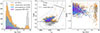 |
Fig. 1. Age distribution (left), Kiel diagram (centre), and age-metallicity coverage (right) for each step of the selection process, before visual inspection. In the centre panel, PARSEC isochrones at different ages and metallicities are shown in grey; at the bottom left, the average error in log g and Teff for the full sample is shown. The peak at 19 Gyr visible in the histogram is due to contaminants (see Sect. 3.1 and Appendix A.1). |
(2) Conservative MSTO-SGB stars cut. As anticipated in Sect. 2, a cut in the Kiel diagram was already made in the age sample to select only MSTO and SGB stars. This selection, though, could be contaminated by stars in different evolutionary stages (low-luminosity giants, MS stars), hidden binaries, or mass-stripped stars (see Appendix A.1 for details). To this end, we adopted a more restrictive selection, already tested in N24, in the log g − Teff plane. This is shown with a solid line in the central panel in Fig. 1, while the resulting sample, of 2148 objects, is shown in orange. This cut was highly effective in suppressing the 19 Gyr peak, suggesting that this overdensity was primarily due to contamination.
(3) Consistency of input–output parameters. Age estimates can also be affected by parameter degeneracies, which may introduce systematic biases. In particular, the age–metallicity degeneracy displayed a clear trend: more metal-poor stars ([M/H]< − 0.5) were systematically shifted towards higher metallicities by 0.1−0.2 dex, while yielding old ages exceeding 18 Gyr. This is shown and discussed in more detail in Appendix A. To mitigate this effect, we imposed a constraint on the maximum allowed discrepancy between the input and output values of [M/H], the first being the results from Guiglion et al. (2024), as anticipated in Sect. 1. We chose a symmetric cut, discarding the 5% tails of the Δ[M/H] distribution, i.e. |Δ[M/H]| < 0.025. Following the same logic, we imposed similar cuts on Teff, |ΔTeff|< 30 K, log g, |Δlog g|< 0.05, and dust extinction, |ΔAV|< 0.1 mag. This further reduced the sample to 1078 stars (see Fig. A.1).
(4) Removing strongly degenerate solutions. Next, we considered the symmetry of the posterior distributions in age and mass as quality indicators as these two parameters are not constrained by Gaussian priors and are therefore more prone to asymmetries or anomalies in their posterior shapes. First, we discarded age measurements for which the asymmetry (difference between the upper and lower uncertainties) exceeded 0.1 Gyr. We then applied a Kolmogorov–Smirnov test to assess how well each posterior probability distribution function (PDF) conformed to a Gaussian, excluding all cases where the probability of deviation from Gaussianity exceeded 99.5%. This reduced the sample to 297 stars.
(5) Visual inspection. As a final step, we visually inspected the corner plots to exclude anomalous cases missed by the previous cuts. This blind inspection, performed without viewing the parameter values, focused on identifying asymmetries or double peaks in the posterior distributions. Based on PDF shape, stars were classified into three quality tiers: great (78 stars, symmetric and clean), good (107 stars, minor tail features), and bad (112 stars, significant asymmetries or almost double peaks), with the latter excluded from the final sample. Examples of this classification process are shown in Appendix A.3.
Finally, we arrived at a refined final sample of 185 stars with precise age determinations, robust stellar parameters, and well-behaved posterior distributions. The ages and masses for these stars are available in an online table, described in Appendix D. Within this set, we also defined a golden sample consisting of the 78 stars that exhibit the highest-quality PDFs. Both samples show a 5% (stat) precision in age and 2% (stat) precision in mass, on average.
The selection favours the more metal-rich part of the parent sample ([M/H]> − 0.5; see right panel in Fig. 1) with low α-enhancement ([α/Fe] < 0.15). This is mainly due to two reasons. First, achieving high-precision age estimates requires very high precision in mass (≲2%), which in turn relies on accurate distances. These can be obtained preferentially in the solar neighbourhood, where metal-poor stars are intrinsically rarer. Second, the stellar parameter determination pipeline, through the hybrid-CNN already mentioned, best performs around solar metallicities, where most of the training sample was (see Guiglion et al. 2024, for details). These considerations inevitably introduce selection effects in terms of metallicity coverage, but they do not compromise the robustness of the final age constraint. Additionally, even though one would expect the oldest stars to be more metal-poor ([M/H] < −1), recent studies (e.g. Trevisan et al. 2011; Anders et al. 2018; Miglio et al. 2021a; Nepal et al. 2024; Borbolato et al. 2025, and references therein) have already shown the existence of old, more metal-rich, low-alpha stars, compatible with a high star formation rate and rapid metal enrichment in the early Milky Way. At high redshift, while direct stellar observations are currently not possible, recent studies of gas phase metallicities have revealed a large dispersion, including super-solar estimates (e.g. Huyan et al. 2025; Deepak et al. 2025). Most stars also show low extinction (AV < 0.5 mag) as the whole final sample is confined within ∼700 pc of the Sun.
In Fig. 2, we show the distribution of the main physical parameters (α-enhancement, metallicity, dust reddening, and mass) versus age for the final and golden sample. The histograms show that our sample does not deviate much from solar values. Considering the final sample, the mean and standard deviation for each quantity are
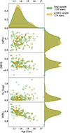 |
Fig. 2. Trends with age of the main parameters: (from bottom to top) mass, dust reddening, overall metallicity, and α-enhancement. On the right the corresponding normalised distributions are shown for each parameter, and at the top the distribution in age. |
![Mathematical equation: $$ \begin{aligned} \langle M/M_\odot \rangle&= 0.88 \pm 0.03\\ \langle [\alpha /\mathrm{Fe}]\rangle&= 0.17 \pm 0.21\\ \langle A_{\rm V}\rangle&= 0.08 \pm 0.04\;\mathrm{mag}\\ \langle [\mathrm{M/H}]\rangle&= -0.24 \pm 0.15. \end{aligned} $$](/articles/aa/full_html/2026/03/aa57038-25/aa57038-25-eq1.gif)
We also observe an inverse correlation between age and mass, with the least massive stars exhibiting the oldest ages. While this trend is expected, it may also hint at potential contamination, particularly in the low-mass tail, where a noticeable peak appears in the age distribution of the golden sample. These stars, with masses as low as 0.8 M⊙, could represent remnants of stars that were originally more massive and that evolved in binary systems that stripped away part of their gas. Recent evidence suggests that the fraction of mass transfer, degenerates, and mergers could represent about ∼20% of Population II stars (Fuhrmann & Chini 2021), so we need to account for this component in the following.
3.2. Systematic effects
When relying on absolute age determination, it is important to account for any systematic effects at play. When performing isochrone fitting, two main sources of systematic uncertainties are involved, the first arising from the choice of stellar models (see e.g. Lebreton et al. 2014; Nsamba et al. 2021, and references therein), the second depending on the potential biases affecting parameters such as metallicity or α-enhancement assumed in the fitting process.
In N24 it is observed how the α-element abundances could be underpredicted for some MSTO stars by up to 0.08 dex, owing to a comparison with common GALAH DR3 (Buder et al. 2021) stars. This little shift, if present, would cause an underestimation of the overall metallicity on which a Gaussian prior is assumed, thus overestimating the derived age. To account for this possible bias, following the approach adopted in N24, we perturbed the assumed [α/Fe] by ±0.1 and found, on average, a shift of ±0.28 Gyr. However, as we discuss above, most of our selected stars have rather low α-enhancements (see Fig. 2).
In terms of stellar models, a positive note is that their difference is minimal for solar-like objects, as all models are calibrated to reproduce observations of the Sun, and our final sample shows properties that deviate very little from solar-like values. Nevertheless, different assumptions (e.g. on the initial helium fraction, mixing length, or treatment of diffusion) can lead to different results.
Here we refer in particular to the arguments presented in Joyce et al. (2023) and Lebreton et al. (2014), which respectively discuss the impact of the mixing length parameter (αML) and of the initial helium fraction (Yi) on the ages of MSTO stars. Adapting their considerations to our case, we estimate that these quantities could introduce systematic shifts of approximately ±1 Gyr and ±0.5 Gyr, respectively, assuming that αML varies in the range 1.6 − 1.9 and that Yi spans 0.269 − 0.283, as commonly adopted among the most widely used stellar evolution models. Summing in quadrature these two contributions, we find a total systematic effect linked to the stellar models of 1.1 Gyr. Further details are discussed in Appendix B.
Finally, we conservatively quantify the total systematic error, combining stellar models and metallicity impact, as the linear sum of the two contributions, totalling 1.4 Gyr. We emphasise that the metallicity impact could be drastically reduced if high-resolution spectroscopy becomes available.
3.3. Identifying the tail of spurious ages
As noted in Sect. 3, the tail towards the oldest ages could be contaminated by stars that lost some mass, causing them to appear artificially older, but also by undetected binaries with unequal mass, as shown in Woody et al. (2025). Because they are close to the physical limit imposed by tU, these spurious solutions should emerge as a secondary distribution at older ages. To test this, we fit a Gaussian mixture model to both the good and golden samples, allowing the data to determine the optimal number of components. Based on the Bayesian and Akaike information criteria, the fit favoured two populations: a narrow peak at 13.4 ± 0.8 Gyr and a broader one at 14.8 ± 1.5 Gyr. Given the presence of this secondary component, we estimated the contamination fraction with a hierarchical Bayesian model implemented through PyMC (details are provided in Appendix C). The fit found a tail of about 11% contaminants, peaking near 14.3 Gyr with a dispersion of 0.8 Gyr. Conservatively, we excluded stars with > 20% contamination probability, 25 in total (11 in the golden sample). The cumulative PDFs of the clean final and golden sample peak at 13.6 ± 1.0 Gyr and 13.6 ± 0.9 Gyr, respectively, confirming no significant difference between the two samples. Hence, we adopted the clean final sample (160 stars) as our reference.
4. Implications for cosmology
4.1. From the stellar ages to the age of the Universe
To convert the stellar ages into constraints on tU we need to take into account the delay, δt, between the Big Bang and the moment these objects formed. As the ages of the oldest objects represent a lower limit to tU, a conservative choice would imply accounting for the smallest possible value for δt. Theoretical models of stellar formation (Galli & Palla 2013; Bromm & Yoshida 2011) and spectroscopically confirmed observations of the most distant galaxies (Curtis-Lake et al. 2023; Carniani et al. 2024) show that the very first stars formed at z ≳ 11 − 14, and not earlier than z ∼ 20 − 30, the expected redshift of formation for Pop III stars. This corresponds to an interval δt of about 0.2−0.4 Gyr.
In Fig. 3 we show the cumulative PDF of our final and golden sample. With lines in the same colours, we report the cumulative distribution obtained by adding the systematic errors in quadrature to each star, as discussed in Sect. 3.2. The final cumulative PDF, shows a mean and standard deviation of
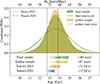 |
Fig. 3. Cumulative posterior distribution in age for the final and golden samples. The distributions including the systematic component of the error are shown as solid lines in the same colours. The upper axis shows the corresponding H0 value, assuming zf = 20. In the lower panel, the age ranges covered by the stars in the final and golden samples and their means are shown in comparison with the oldest GCs (> 12.5 Gyr) in Valcin et al. (2025) and the oldest bulge GCs in Souza et al. (2024). |

Also accounting for the minimum formation time for these stars, this produces a lower limit to the age of the Universe,

which would increase should these stars have formed at z < 11.
In the upper axis of Fig. 3, the values of the Hubble constant H0 are also reported assuming a redshift of formation for the sample zf = 20. Under these assumptions, the lower limit on the age of the Universe translates, in terms of H0, into

and would further decrease by 1.2 km/s/Mpc assuming zf = 11. For comparison, the two values currently leading the Hubble tension (Planck Collaboration VI 2020; Riess et al. 2022) are also shown as dashed lines. We note that the assumptions made here to connect H0 and tU are commonly adopted, but represent a particular case. The relation between H0 and tU can be influenced by different factors, especially the value assumed for Ωm, but also by the cosmological model in general. In Sect. 4.2 we discuss this aspect in more detail. Regardless of the implications on the value of H0, the sample identified in this work provides important and direct constraints on the age of the Universe itself, representing an observational anchor point to any cosmological model.
Considering the single PDFs of the 160 stars in the final sample (excluding, for now, systematic uncertainties) and shifting them by the minimum possible delay (0.2 Gyr), we find that at the 90% confidence level (CL), 70 stars indicate an age of the Universe older than 13 Gyr, and 29 stars suggest an age older than 13.5 Gyr, while no star exceeds 14.1 Gyr at 90% CL. Notably, shifting this upper envelope down to ages below 13 Gyr would require applying nearly the entire systematic error budget, implying that such a substantial reduction in the inferred ages is only achievable under the most conservative assumptions. While this may be plausible for the [α/Fe] estimation component (0.3 Gyr in the error budget), there is no evidence favouring stellar models that predict systematically younger ages. On the contrary, considering models with higher αML or lower Yi (see Appendix B for details), age estimates could easily increase by 1 Gyr.
The results of this work are also complemented and supported by independent age estimations obtained for very old GCs, such as the ones in Valcin et al. (2025) and the bulge GCs in Souza et al. (2024). In the lower panel of Fig. 3 we show the age ranges and mean values from these two studies restricted to clusters older than 12.5 Gyr, consistent with our selection. The figure highlights how the tail of the oldest GCs overlaps with the age distribution of our sample. Although the stellar models adopted in the two studies differ from those used here, the age ranges of the oldest GCs vary by less than 1 Gyr; the average ages differ by only ∼0.52 Gyr (Valcin et al. 2025) and ∼0.7 Gyr (Souza et al. 2024). Remarkably, both samples show metallicities comparable to those in our sample, reinforcing the conclusion that such old ages are achievable even at these metallicities, thus supporting a scenario of rapid early formation.
4.2. Alternative cosmological assumptions
In Fig. 4 we show how the upper axis of Fig. 3 changes when changing the values of the matter density parameter ΩM and of the assumed redshift of formation for these stars, zf. The histograms show the 10th percentile distribution in age of the final and golden samples, including the systematic component of the error for each star. All panels share the same lower horizontal age axis, while the upper one, in H0, varies depending on the assumed value of Ωm and zf. This allows us to show how the distribution found in this work compares with the measurements from Planck Collaboration VI (2020) and Riess et al. (2022), represented by a dashed and a dash-dotted line, respectively, at varying cosmological assumptions. The percentages reported in each panel, next to these lines, show the fraction of stars older than the respective ages of the Universe at 90% CL (stat+syst), thus pointing to a lower H0 value at 90% CL.
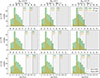 |
Fig. 4. Distribution of the 10th percentile in age for the clean final (green) and golden (gold) samples. In each panel, the top axis shows the corresponding H0 values assuming a flat ΛCDM and a different value of Ωm and zf. The rows from top to bottom set zf = 10, 20, ∞; the columns from left to right fix Ωm = 0.25, 0.3, 0.35. The dashed and dash-dotted lines report the H0 measurements from Riess et al. (2022) and Planck Collaboration VI (2020), respectively. Next to each one the percentage of stars in the final (green) and golden (gold) samples pointing to a lower H0 at 90% CL (stat+syst) are reported. |
The setting adopted in Fig. 3 corresponds to that in the central panel in Fig. 4. Overall, this shows how zf and Ωm act when translating the age of the oldest objects into H0: the higher the assumed zf, the higher the retrieved H0, while the opposite is true for Ωm. In the context of the Hubble tension, this shows that the sample in this work points to H0 lower than the CMB value only when Ωm = 0.35 and zf = 10. Instead, compared to Riess et al. (2022), all configurations with Ωm ≥ 0.3 show at least 4% of stars, up to 48%, pointing to a lower value of H0 at 90% CL. The only configurations showing no tensions with any of the two measurements are the ones with Ωm = 0.25.
5. Conclusions
In this paper, the ages of the oldest stars from Gaia DR3 are used to constrain the age of the Universe, tU. It was the first attempt to use the ages of single stars as cosmic clocks with a statistically significant sample.
We considered the ∼200 000 stars from N24, with ages and masses estimated via the Bayesian code StarHorse, but allowing ages to vary up to 20 Gyr without a cosmological prior. We selected the ∼3000 stars older than 12.5 Gyr with age uncertainties below 1 Gyr. Through a careful selection process including cuts in the Kiel diagram, stellar parameter quality, symmetry of posterior distributions, and a final visual inspection, we removed stars with potentially biased age estimates, especially those skewed to older values, to obtain a conservative and robust lower limit on stellar ages and thus on tU.
We identified two subpopulations in age, one at ∼13.7 with very little dispersion (∼0.3 Gyr) and an older one at ∼14.8 Gyr with a dispersion of ∼0.8 Gyr. Assuming a fraction of stars could be composed of older contaminants (e.g. mass-stripped stars, binaries) that appear older than they are, we conservatively excluded all stars belonging to the second peak (∼11%).
The final sample counts 160 stars, with a cumulative posterior distribution peaking at 13.6 ± 1.0 (stat) ± 1.3 (syst) Gyr. The main source of systematic error comes from stellar models. Accounting for the minimum possible delay between the Big Bang and the formation of these stars, 0.2 Gyr at zf = 20, we derive a conservative lower limit on tU, and an upper limit on H0:
Considering them one by one, 70 stars indicate an age of the Universe older than 13 Gyr, while no star exceeds 14.1 Gyr at 90% CL (stat). Notably, the full systematic error budget would be needed, consistently pointing towards younger ages, to move this drop to 13 Gyr or less.
In conclusion, this work shows how the ages of single stars derived from isochrone fitting can provide stringent constraints on tU, and a robust anchor point to any cosmological model. While this represents a significant first step, future data releases from Gaia will enable similar analyses on larger stellar samples with improved precision. Furthermore, the accuracy and reliability of age determinations can be improved by obtaining metallicities from high-resolution spectroscopy, minimising, at the same time, the systematic error due to the α-enrichment. However, only with missions such as Haydn (Miglio et al. 2021b) will it be possible to achieve accurate ages for field stars in the MW.
Data availability
Table D.1 is available at the CDS via https://cdsarc.cds.unistra.fr/viz-bin/cat/J/A+A/707/A111
Acknowledgments
We thank the anonymous referee for their valuable and constructive feedback, which helped us improve the robustness of our findings. We thank Andrea Miglio, Arman Khalatyan, and the e-science department of AIP for their contributions to this paper. Part of this project was conducted at AIP within the Marco Polo program. ET acknowledges COST Action CA21136 – “Addressing observational tensions in cosmology with systematics and fundamental physics (CosmoVerse)”, supported by COST (European Cooperation in Science and Technology). CC acknowledges the Astronomy Department of the University of São Paulo and FAPESP. MM acknowledges the financial contribution from the grant PRIN-MUR 2022 2022NY2ZRS 001 “Optimizing the extraction of cosmological information from Large Scale Structure analysis in view of the next large spectroscopic surveys” supported by Next Generation EU. MM and AC acknowledge support from the grant ASI n. 2024-10-HH.0 “Attività scientifiche per la missione Euclid – fase E”. This work was partially funded by the Spanish MICIN/AEI/10.13039/501100011033 and by the “ERDF A way of making Europe” funds by the European Union through grant RTI2018-095076-B-C21 and PID2021-122842OB-C21, and the Institute of Cosmos Sciences University of Barcelona (ICCUB, Unidad de Excelencia ‘María de Maeztu’) through grant CEX2019-000918-M. FA acknowledges financial support from MCIN/AEI/10.13039/501100011033 through a RYC2021-031638-I grant co-funded by the European Union NextGenerationEU/PRTR.
References
- Abdalla, E., Abellán, G. F., Aboubrahim, A., et al. 2022, J. High Energy Astrophys., 34, 49 [NASA ADS] [CrossRef] [Google Scholar]
- Amard, L., Palacios, A., Charbonnel, C., et al. 2019, A&A, 631, A77 [NASA ADS] [CrossRef] [EDP Sciences] [Google Scholar]
- Anders, F., Chiappini, C., Santiago, B. X., et al. 2018, A&A, 619, A125 [NASA ADS] [CrossRef] [EDP Sciences] [Google Scholar]
- Anders, F., Khalatyan, A., Queiroz, A. B. A., et al. 2022, A&A, 658, A91 [NASA ADS] [CrossRef] [EDP Sciences] [Google Scholar]
- Borbolato, L., Rossi, S., Perottoni, H. D., et al. 2025, ApJ, 994, 126 [Google Scholar]
- Boylan-Kolchin, M., & Weisz, D. R. 2021, MNRAS, 505, 2764 [NASA ADS] [CrossRef] [Google Scholar]
- Bressan, A., Marigo, P., Girardi, L., et al. 2012, MNRAS, 427, 127 [NASA ADS] [CrossRef] [Google Scholar]
- Bromm, V., & Yoshida, N. 2011, ARA&A, 49, 373 [CrossRef] [Google Scholar]
- Buder, S., Sharma, S., Kos, J., et al. 2021, MNRAS, 506, 150 [NASA ADS] [CrossRef] [Google Scholar]
- Carniani, S., Hainline, K., D’Eugenio, F., et al. 2024, Nature, 633, 318 [CrossRef] [Google Scholar]
- Cimatti, A., & Moresco, M. 2023, ApJ, 953, 149 [NASA ADS] [CrossRef] [Google Scholar]
- Curtis-Lake, E., Carniani, S., Cameron, A., et al. 2023, Nat. Astron., 7, 622 [NASA ADS] [CrossRef] [Google Scholar]
- Deepak, S., Howk, J. C., Lehner, N., & Péroux, C. 2025, ApJ, 987, 199 [Google Scholar]
- Di Valentino, E., Anchordoqui, L. A., Akarsu, Ö., et al. 2021, Astropart. Phys., 131, 102607 [NASA ADS] [CrossRef] [Google Scholar]
- Di Valentino, E., Said, J. L., Riess, A., et al. 2025, Phys. Dark Univ., 49, 101965 [Google Scholar]
- Dotter, A., Conroy, C., Cargile, P., & Asplund, M. 2017, ApJ, 840, 99 [Google Scholar]
- Fuhrmann, K., & Chini, R. 2021, MNRAS, 501, 4903 [NASA ADS] [CrossRef] [Google Scholar]
- Gaia Collaboration (Prusti, T., et al.) 2016, A&A, 595, A1 [NASA ADS] [CrossRef] [EDP Sciences] [Google Scholar]
- Gaia Collaboration (Vallenari, A., et al.) 2023, A&A, 674, A1 [NASA ADS] [CrossRef] [EDP Sciences] [Google Scholar]
- Galli, D., & Palla, F. 2013, ARA&A, 51, 163 [NASA ADS] [CrossRef] [Google Scholar]
- Guiglion, G., Nepal, S., Chiappini, C., et al. 2024, A&A, 682, A9 [NASA ADS] [CrossRef] [EDP Sciences] [Google Scholar]
- Huyan, J., Kulkarni, V. P., Poudel, S., et al. 2025, ApJ, 991, 228 [Google Scholar]
- Jimenez, R., Cimatti, A., Verde, L., Moresco, M., & Wandelt, B. 2019, JCAP, 2019, 043 [CrossRef] [Google Scholar]
- Joyce, M., Johnson, C. I., Marchetti, T., et al. 2023, ApJ, 946, 28 [NASA ADS] [CrossRef] [Google Scholar]
- Kamionkowski, M., & Riess, A. G. 2023, Ann. Rev. Nucl. Part. Sci., 73, 153 [NASA ADS] [CrossRef] [Google Scholar]
- Korn, A. J., Grundahl, F., Richard, O., et al. 2007, ApJ, 671, 402 [NASA ADS] [CrossRef] [Google Scholar]
- Krauss, L. M., & Chaboyer, B. 2003, Science, 299, 65 [Google Scholar]
- Lebreton, Y., Goupil, M. J., & Montalbán, J. 2014, EAS Publ. Ser., 65, 99 [CrossRef] [EDP Sciences] [Google Scholar]
- Marigo, P., Girardi, L., Bressan, A., et al. 2017, ApJ, 835, 77 [Google Scholar]
- Miglio, A., Chiappini, C., Mackereth, J. T., et al. 2021a, A&A, 645, A85 [NASA ADS] [CrossRef] [EDP Sciences] [Google Scholar]
- Miglio, A., Girardi, L., Grundahl, F., et al. 2021b, Exp. Astron., 51, 963 [NASA ADS] [CrossRef] [Google Scholar]
- Moresco, M., Amati, L., Amendola, L., et al. 2022, Liv. Rev. Relat., 25, 6 [NASA ADS] [Google Scholar]
- Nepal, S., Chiappini, C., Queiroz, A. B., et al. 2024, A&A, 688, A167 [NASA ADS] [CrossRef] [EDP Sciences] [Google Scholar]
- Nsamba, B., Moedas, N., Campante, T. L., et al. 2021, MNRAS, 500, 54 [Google Scholar]
- O’Malley, E. M., Gilligan, C., & Chaboyer, B. 2017, ApJ, 838, 162 [CrossRef] [Google Scholar]
- Planck Collaboration VI. 2020, A&A, 641, A6 [NASA ADS] [CrossRef] [EDP Sciences] [Google Scholar]
- Price-Whelan, A. M., Hogg, D. W., Rix, H.-W., et al. 2020, ApJ, 895, 2 [NASA ADS] [CrossRef] [Google Scholar]
- Queiroz, A. B. A., Anders, F., Santiago, B. X., et al. 2018, MNRAS, 476, 2556 [Google Scholar]
- Queiroz, A. B. A., Anders, F., Chiappini, C., et al. 2023, A&A, 673, A155 [NASA ADS] [CrossRef] [EDP Sciences] [Google Scholar]
- Riess, A. G., Yuan, W., Macri, L. M., et al. 2022, ApJ, 934, L7 [NASA ADS] [CrossRef] [Google Scholar]
- Santiago, B. X., Brauer, D. E., Anders, F., et al. 2016, A&A, 585, A42 [NASA ADS] [CrossRef] [EDP Sciences] [Google Scholar]
- Skrutskie, M. F., Cutri, R. M., Stiening, R., et al. 2006, AJ, 131, 1163 [NASA ADS] [CrossRef] [Google Scholar]
- Soderblom, D. R. 2010, ARA&A, 48, 581 [Google Scholar]
- Souza, S. O., Libralato, M., Nardiello, D., et al. 2024, A&A, 690, A37 [NASA ADS] [CrossRef] [EDP Sciences] [Google Scholar]
- Tomasetti, E., Moresco, M., Lardo, C., Cimatti, A., & Jimenez, R. 2025, A&A, 696, A98 [NASA ADS] [CrossRef] [EDP Sciences] [Google Scholar]
- Trevisan, M., Barbuy, B., Eriksson, K., et al. 2011, A&A, 535, A42 [NASA ADS] [CrossRef] [EDP Sciences] [Google Scholar]
- Vagnozzi, S., Pacucci, F., & Loeb, A. 2022, J. High Energy Astrophys., 36, 27 [NASA ADS] [CrossRef] [Google Scholar]
- Valcin, D., Bernal, J. L., Jimenez, R., Verde, L., & Wandelt, B. D. 2020, JCAP, 2020, 002 [Google Scholar]
- Valcin, D., Jimenez, R., Verde, L., Bernal, J. L., & Wandelt, B. D. 2021, JCAP, 2021, 017 [CrossRef] [Google Scholar]
- Valcin, D., Jimenez, R., Seljak, U., & Verde, L. 2025, JCAP, 2025, 030 [Google Scholar]
- Woody, T., Conroy, C., Cargile, P., et al. 2025, ApJ, 978, 152 [Google Scholar]
Adopting a more stringent uncertainty cut of 0.75 Gyr would have reduced the parent sample to roughly one-third of its current size, while decreasing the final age estimate by only 0.1 Gyr.
Peculiar GCs showing a spread in metallicity (namely NGC 5286, NGC 5139, and NGC 7089) were removed from the sample.
Wide binaries are already excluded from the original selection from N24.
Appendix A: Sample selection
A.1. Conservative cut in the Kiel diagram
Following what was already presented in N24, we adopted the following cut in log g − Teff plane,
 (A.1)
(A.1)
and selected a restricted area in the Kiel diagram. The cut in log g < 4.1, in particular, is what impacted most on the parent sample and removed most of the stars older than 18 Gyr. Above this threshold, as is clear from the central panel in Fig. 1, we would select stars that overlap with the turn-off, but potentially still in MS. The simple scatter of MS stars, but also unresolved binary systems3, could imply a lower surface gravity (see e.g. Price-Whelan et al. 2020; Anders et al. 2022, for a discussion on binarity). This has a different effect on the resulting age depending on the position in the diagram: above log g ∼ 4.1, around the turn-off, this can drag the age to much older values because isochrones of different age around the MS are very close by; below log g ∼ 4.1, above the turn-off, instead, such upwards shift would typically result in a younger age, but with a much less dramatic effect because the isochrones of different age are distinct parallel lines after the turn-off. We underline that by selecting this region of the Kiel diagram, we are not removing by definition the oldest solutions: isochrones of ages up to 20 Gyr are still included in the selected area, as visible in the central panel of Fig. 1.
A.2. Consistency of input–output metallicity
In Figure A.1, the difference is shown between the StarHorse overall metallicities and the values from Guiglion et al. (2024), used as priors, for the sample selected after the conservative cut (2148 stars). It clearly highlights how the oldest ages, above 18 Gyr, are all related to an overestimation of the input metallicity by up to 0.2 dex. From the histogram on the right, it is also clear that these stars are just a very small fraction, less than 5% of the entire population. The dashed lines show the cut that we adopted to remove these stars and keep only the most stable results, in which the code did not deviate much from the metallicity prior.
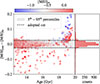 |
Fig. A.1. Discrepancy in [M/H] between StarHorse’s output and the measurements from Guiglion et al. (2024), used as a prior. |
A.3. Visual inspection
In Fig. A.2, three corner plots are shown for stars representing different levels of quality in their posterior probability distribution functions (PDFs) for mass and age. The top panel illustrates one of the best cases, characterised by a Gaussian and symmetric distribution in both parameters. The middle panel presents a good-quality PDF, with a single peak and an overall Gaussian-like shape, but slight asymmetries appear in the tails beyond the 1σ range. The bottom panel shows a poor-quality fit that was excluded from the final sample. Although the main peak is visible, a secondary peak appears at higher masses and lower ages, close enough to the main one that it was not flagged in earlier selection steps. This bimodality suggests a non-negligible probability assigned to a different solution, reducing the robustness of the fit for the purposes of this study.
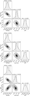 |
Fig. A.2. Examples of corner plots of different quality, classified in the visual inspection phase into best, good, and bad PDFs. |
Appendix B: Systematics: Stellar models
Carefully assessing the impact of the stellar models is a non-trivial task, but we can derive a realistic estimation of this systematic component following the results found in previous works.
First, we followed the approach presented in (Joyce et al. 2023). The authors focus on the impact of the convective mixing length parameter, αML, that they argue is likely dominating the systematic error budget linked to the stellar models, and they vary this parameter on a wide range – 1.4 to 2.3 when considering MSTO and SGB (see Fig. 11 in Joyce et al. 2023). To mimic this variation, they perform a Monte Carlo simulation perturbing the set of isochrones by 200 K in Teff and 0.17 dex in log g, on average, finding an average shift in ages of 1-2 Gyr, where a higher αML produces older ages. In order to adapt this analysis to our case, we need to make three considerations.
First, the range adopted for αML is very wide if compared to the typically used values in most stellar models, ranging mostly from 1.6 to 1.9 (see e.g. Table 4 in Amard et al. 2019, for a summary). The models used in this work, PARSEC, set αML = 1.74 − 1.77, which is in the middle of this interval.
Second, the Kiel diagram area covered by the final sample in this work is confined between 5400-5700 K in Teff and 3.8-4.1 in log g, where the effect of αML is minimal and fully horizontal (i.e. it produces only a shift in Teff). Considering the full range 1.4-2.3, this produces shifts of ±100 − 150 K from the mean value, while considering the most used range 1.6-1.9, this implies fluctuations of ±30 − 50 K.
Third, the uncertainties in Teff, log g, and metallicity in this work are up to 4-5 times smaller than the ones considered in (Joyce et al. 2023).
Owing to these considerations, we conclude that the lower bound of the interval identified in Joyce et al. (2023) – 1 Gyr – is an overly conservative choice to account for this model-related systematic component in this work.
Systematic uncertainties may also arise from discrepancies between the actual stellar helium content and the values assumed in model grids (see Lebreton et al. 2014; Nsamba et al. 2021, for a detailed discussion). These studies show that adopting different assumptions for the initial helium content – either reading it as a free parameter or raising it via a ΔY/ΔZ relation – can introduce systematic effects of the order of a few percent in mass and, therefore, in age. However, for our sample, most stars have metallicities close to solar, so their helium abundances are expected to be similar to those assumed in standard stellar models (solar mixture).
Quantifying the impact of varying the initial helium abundance Yi on turn-off ages is not straightforward, but previous studies allow us to obtain a reasonable estimate. In particular, Lebreton et al. (2014) explored the sensitivity of stellar ages to Yi by adopting a reference value Yi = 0.28 and considering two extreme cases, Yi = 0.31 and Yi = 0.25 (see Fig. 22 in Lebreton et al. 2014). Their results clearly show that increasing Yi leads to a younger inferred age, while a lower initial helium abundance produces the opposite effect. Assuming that the response is approximately linear over this interval, a variation of δYi = ±0.01 corresponds to an age shift of δage ≈ ∓0.75 Gyr.
This range in helium is relatively large when compared with the values adopted in most widely used stellar evolution grids, where Yi typically lies in the narrow interval 0.269–0.283 (see Table 4 in Amard et al. 2019). Such a spread corresponds to a total δYi ≃ 0.015, implying an overall uncertainty of roughly 1 Gyr in the turn-off age. Since the PARSEC models used in this work adopt values of Yi near the middle of this range, we estimate a final age uncertainty of about ±0.5 Gyr associated with plausible variations in the initial helium content.
Another potential systematic effect linked to the stellar models is the one of atomic diffusion, causing the exterior of the star to appear more metal-poor with respect the internal, initial value of metallicity (see e.g. Korn et al. 2007). The effect of diffusion is, anyway, already included in the PARSEC models, as explained in Anders et al. (2022), Sect. 3.1.4. This allows the code to account for possible changes in the surface metallicity during stellar evolution, for example the decrease caused by element diffusion before and around the turn-off (see Marigo et al. 2017). Additionally, even if the current knowledge of this process is still incomplete, it should be less and less relevant moving towards older ages and to metallicities around solar (see Fig. 3 in Dotter et al. 2017). For this reason, we decided not to add another source of systematic error owing to this effect.
Finally, summing in quadrature the systematic effects discussed here, we end up with a total systematic uncertainty linked to the stellar models of 1.1 Gyr.
Appendix C: Removing potential contaminants
In order to identify the possible contamination fraction of older stars that lost their mass, or undetected binaries, we fit our distribution as the combination of a true and a contaminant population, following the approach described in detail in Miglio et al. (2021a).
Assuming a combination of two normally distributed samples, the first with mean μ and intrinsic dispersion σ, the second represented by a fraction, fc, with mean μc and dispersion σc, the model can be summarised by the following likelihood function:
![Mathematical equation: $$ \begin{aligned} \begin{aligned} \mathcal{L} (\mathbf \theta \mid \mathbf x,\sigma _x ) = \prod _{i = 1}^N&\Bigl [(1-f_c)\,\mathcal{TN} \bigl (\mu ,\;\sigma ^2 + \sigma _{x,i}^2,\,12,\,20\bigr )\\&\quad +\,f_c\,\mathcal{TN} \bigl (\mu _c,\;\sigma _c^2 + \sigma _{x,i}^2,\,12,\,20\bigr )\Bigr ]. \end{aligned} \end{aligned} $$](/articles/aa/full_html/2026/03/aa57038-25/aa57038-25-eq7.gif) (C.1)
(C.1)
Here 𝒯𝒩(μ, σ2, a, b) is a normal distribution truncated in the range [a,b] and (x, σx) is the set of age measurements and associated errors.
We adopt uniform, wide, priors on μ and μc, respectively in the range 0–20 Gyr and 13–20 Gyr. On σ and σc, we adopt lognormal priors, centred at 1 Gyr with standard deviation 0.5 Gyr. For the contamination fraction, fc, we use a β-function with parameters a = 2 and b = 8.
For the sampling of the posterior probability distribution, performed in PyMC with the No-U-Turn Samples (NUTS), we use four chains of 2000 steps, after performing 1000 burn-in steps, totalling 8000 samples.
The joint posterior distribution for the five parameters is shown in Fig. B.1, where the inset shows the decomposition in the final sample distribution. The median values and 68% contours for each parameter are the following:
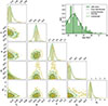 |
Fig. B.1. Joint posterior distribution of the five parameters included in the model reproducing the age distribution. Contours obtained with the final sample are shown in green, and in yellow for the golden sample. The inset shows the age distribution of the final sample and the two components resulting from the fit. |
We then removed from the sample all stars with a probability of being contaminants higher than 20%, computed as
 (C.2)
(C.2)
where xi is a single age measurement, and 𝒩(a; b, c) is the value of a normal distribution with mean b and sigma c evaluated at a. For each star, when possible, we computed this probability using the best-fit values obtained from fitting both the final sample and the golden sample, as listed in Fig. B.1. This process led us to discard 11 stars from the golden sample and 25 stars from the final sample, with all contaminants present in the first also identified in the second.
We note that we also tested how the results would change by adopting Lorentzian fitting functions instead of a Gaussian ones. The Lorentzian distribution, indeed, presents extended tails that, in some cases, better reflect the shape of age PDFs in the sample. Although this led to a slightly smaller estimated fraction of contaminants (∼5%), the presence of a secondary low-weight outlier component remained. Moreover, the position of the main peak was found to be fully consistent with that obtained using Gaussians. To ensure the robustness of the cosmological results, we conservatively chose to reject the higher fraction of potential contaminants identified with the Gaussian fits, as this represents the most cautious approach to prevent any residual anomalies in the sample.
Appendix D: Description of online table
StarHorse derived age, mass, and respective uncertainties for the 185 clean sample stars.
All Tables
StarHorse derived age, mass, and respective uncertainties for the 185 clean sample stars.
All Figures
|
Fig. 1. Age distribution (left), Kiel diagram (centre), and age-metallicity coverage (right) for each step of the selection process, before visual inspection. In the centre panel, PARSEC isochrones at different ages and metallicities are shown in grey; at the bottom left, the average error in log g and Teff for the full sample is shown. The peak at 19 Gyr visible in the histogram is due to contaminants (see Sect. 3.1 and Appendix A.1). |
| In the text | |
|
Fig. 2. Trends with age of the main parameters: (from bottom to top) mass, dust reddening, overall metallicity, and α-enhancement. On the right the corresponding normalised distributions are shown for each parameter, and at the top the distribution in age. |
| In the text | |
|
Fig. 3. Cumulative posterior distribution in age for the final and golden samples. The distributions including the systematic component of the error are shown as solid lines in the same colours. The upper axis shows the corresponding H0 value, assuming zf = 20. In the lower panel, the age ranges covered by the stars in the final and golden samples and their means are shown in comparison with the oldest GCs (> 12.5 Gyr) in Valcin et al. (2025) and the oldest bulge GCs in Souza et al. (2024). |
| In the text | |
|
Fig. 4. Distribution of the 10th percentile in age for the clean final (green) and golden (gold) samples. In each panel, the top axis shows the corresponding H0 values assuming a flat ΛCDM and a different value of Ωm and zf. The rows from top to bottom set zf = 10, 20, ∞; the columns from left to right fix Ωm = 0.25, 0.3, 0.35. The dashed and dash-dotted lines report the H0 measurements from Riess et al. (2022) and Planck Collaboration VI (2020), respectively. Next to each one the percentage of stars in the final (green) and golden (gold) samples pointing to a lower H0 at 90% CL (stat+syst) are reported. |
| In the text | |
|
Fig. A.1. Discrepancy in [M/H] between StarHorse’s output and the measurements from Guiglion et al. (2024), used as a prior. |
| In the text | |
|
Fig. A.2. Examples of corner plots of different quality, classified in the visual inspection phase into best, good, and bad PDFs. |
| In the text | |
|
Fig. B.1. Joint posterior distribution of the five parameters included in the model reproducing the age distribution. Contours obtained with the final sample are shown in green, and in yellow for the golden sample. The inset shows the age distribution of the final sample and the two components resulting from the fit. |
| In the text | |
Current usage metrics show cumulative count of Article Views (full-text article views including HTML views, PDF and ePub downloads, according to the available data) and Abstracts Views on Vision4Press platform.
Data correspond to usage on the plateform after 2015. The current usage metrics is available 48-96 hours after online publication and is updated daily on week days.
Initial download of the metrics may take a while.