| Issue |
A&A
Volume 685, May 2024
|
|
|---|---|---|
| Article Number | L12 | |
| Number of page(s) | 7 | |
| Section | Letters to the Editor | |
| DOI | https://doi.org/10.1051/0004-6361/202450067 | |
| Published online | 20 May 2024 | |
Letter to the Editor
The CO-dark molecular gas in the cold H I arc
1
Institut de Radioastronomie Millimetrique, 300 Rue de la Piscine, 38400 Saint-Martin-d’Hères, France
e-mail: luo@iram.fr
2
CAS Key Laboratory of FAST, National Astronomical Observatories, Chinese Academy of Sciences, Beijing 100101, PR China
3
University of Chinese Academy of Sciences, Beijing 100049, PR China
4
School of Astronomy and Space Science, Nanjing University, Nanjing 210093, PR China
5
Key Laboratory of Modern Astronomy and Astrophysics (Nanjing University), Ministry of Education, Nanjing 210093, PR China
6
Research Center for Astronomical Computing, Zhejiang Laboratory, Hangzhou 311100, PR China
7
Department of Physics, Anhui Normal University, Wuhu, Anhui 241002, PR China
Received:
22
March
2024
Accepted:
3
May
2024
The CO-dark molecular gas (DMG), which refers to the molecular gas not traced by CO emission, is crucial for the evolution of the interstellar medium (ISM). While the gas properties of DMG have been widely explored in the Solar neighborhood, whether or not they are similar in the outer disk regions of the Milky Way is still not well understood. In this Letter, we confirm the existence of DMG toward a cold H I arc structure at 13 kpc away from the Galactic center with both OH emission and H I narrow self-absorption (HINSA). This is the first detection of HINSA in the outer disk region, in which the HINSA fraction (NHINSA/NH2 = 0.022 ± 0.011) is an order of magnitude higher than the average value observed in nearby evolved dark clouds, but is consistent with that of the early evolutionary stage of dark clouds. The inferred H2 column density from both extinction and OH emission (NH2 ≈ 1020 cm−2) is an order of magnitude higher than previously estimated. Although the ISM environmental parameters are expected to be different between the outer Galactic disk regions and the Solar neighborhood, we find that the visual extinction (AV = 0.19 ± 0.03 mag), H2-gas density (nH2 = 91 ± 46 cm−3), and molecular fraction (58% ± 28%) of the DMG are rather similar to those of nearby diffuse molecular clouds. The existence of DMG associated with the expanding H I supershell supports a scenario where the expansion of supershells may trigger the formation of molecular clouds within a crossing timescale of the shock wave (∼106 yr).
Key words: ISM: abundances / ISM: clouds / evolution / ISM: molecules
© The Authors 2024
 Open Access article, published by EDP Sciences, under the terms of the Creative Commons Attribution License (https://creativecommons.org/licenses/by/4.0), which permits unrestricted use, distribution, and reproduction in any medium, provided the original work is properly cited.
This article is published in open access under the Subscribe to Open model. Subscribe to A&A to support open access publication.
1. Introduction
The recycling between interstellar matter and stars is important for understanding star formation and galaxy evolution. H I and H2 are the two most important constituents of the interstellar medium (ISM). While H I can be detected directly by the 21 cm emission line (McKee & Ostriker 1977; Dickey & Lockman 1990; Heiles & Troland 2003; Kalberla & Kerp 2009), H2 cannot be detected directly in emission in the cold environment (e.g., 15 K of molecular clouds) because of the large energy level spacing and weak transition strengths. CO has been used extensively to probe the morphology and physical properties of cold molecular gas over the past half-century (Wilson et al. 1970; Dame et al. 2001; Bolatto et al. 2013).
Growing evidence from γ-ray (e.g., EGRET, Fermi, Grenier et al. 2005; Remy et al. 2017) and dust thermal emission (e.g., Planck, Planck Collaboration XIX 2011) over the past 20 years shows that nearly half of the total neutral gas cannot be traced by H I and CO emission. Studies focusing on spectral lines (e.g., spectra of C+, OH, HCO+) further strengthen the hypothesis that the “unseen” gas is mostly CO-dark molecular gas (DMG, Pineda et al. 2013; Lee et al. 2015; Li et al. 2018; Luo et al. 2020; Busch et al. 2021; Rybarczyk et al. 2022).
DMG is most likely to exist in the low-to-intermediate extinction range (AV: 0.2−2 mag), where the cloud is going through a H I-to-H2 transition phase (Seifried et al. 2020). The fraction of DMG increases monotonically with Galactocentric distance (RGC, Pineda et al. 2013), which is consistent with simulations that show that the fraction of DMG decreases with metallicity (Hu et al. 2021). However, the threshold (e.g., AV, nH) at which H I transforms into H2 in the outer disk region is still unclear.
An extremely cold (Tkin down to 10 K), extended (spatial scale L ∼ 2 kpc), and massive (M ∼ 1.9 × 10⁷ M⊙) H I arc structure (red curves in Fig. 1) was found through H I self-absorption (HISA) signatures without associated CO emission (Knee & Brunt 2001). This structure is located in the northern rim of the expanding supershell GSH139-03-69 (RGC ∼ 16 kpc1, Heiles 1979), but is not supposed to exist according to the classical ISM phase models (Field et al. 1969; McKee & Ostriker 1977). As the cooling of H I at such low temperatures is extremely difficult, the H I arc structure could either be in an unstable adiabatic expansion (Sahai & Nyman 1997; Sahai et al. 2013), or be coexistent with unseen DMG.
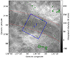 |
Fig. 1. H I integrated intensity (background gray scale) from the Canadian Galactic Plane Survey (CGPS, Taylor et al. 2003) and CO integrated intensity (green contours, 0.4 K km s−1 × (3, 5, 10)) from the Outer Galaxy Survey (OGS, Heyer et al. 1998). The integrated velocity range is −80 to −73 km s−1 for both H I and CO. The H I arc is denoted by the red curves. The yellow square denotes the position where the inferred H I spin temperature is ∼10 K in Knee & Brunt (2001). The blue cross denotes the H I pointing observations, and the blue square is the region mapped in OH. |
In this Letter, we present high-sensitivity and high-spectral-resolution H I observations with the Five-hundred-meter Aperture Spherical Telescope (FAST), and OH observations with the Robert C. Byrd Green Bank Telescope (GBT) toward the arc structure. The H I narrow self-absorption (HINSA) feature and the OH emission confirm the existence of DMG within the H I arc. We highlight the similar physical conditions and H I-to-H2 transition for both nearby clouds and outer disk regions, and the potential of HINSA to probe the DMG properties in future works.
2. Observations
2.1. FAST H I observations
Single-pointing H I observations (blue cross in Fig. 1) were made using the central beam of the 19-beam receiver of FAST – with the total power ON mode – in December 2019 (PI: Ningyu Tang). The rest frequency for the H I observation is 1420.2058 MHz and the spectral resolution is 473 Hz, corresponding to a velocity resolution of 0.1 km s−1 at 1.4 GHz. The system temperature Tsys is 22 K and the integration time is 600 s. The root mean square (rms) of the H I spectrum (in TA units) is 0.054 K per 0.1 km s−1. The main beam efficiency of η = 0.87 was adopted to convert TA into brightness temperature Tmb for the FAST central beam (Tang et al. 2020).
2.2. GBT OH observations
We performed mapping observations of four OH Λ-doubling lines in the 2Π3/2, J = 3/2 energy level from Feb. 10, 2022 to March 12, 2022, using the L-band receiver on board the GBT in on-the-fly mode (Project ID: 22A-228, PI: Gan Luo). The observed map is centered at right ascension (RA) = 02h50m40.1s and declination (Dec) = +61°34′58.3″, covering a region of 1.7 sq. deg. (blue square in Fig. 1). The observations used the VEGAS backend with the total power ON mode. The spectral resolution of OH is 358 Hz (0.064 km s−1 at 1667 MHz). We smoothed the data to a velocity resolution of 0.25 km s−1 to obtain a higher signal-to-noise ratio (S/N). The system temperature is ∼19 K, and the beam efficiency is ∼71% for OH observations. The datacube was regridded to a pixel size of 3.1′. The total observing time is 12 h, resulting in an rms noise level of ∼0.02 K per velocity channel per pixel.
2.3. Archive FCRAO CO (1–0) data
The 12CO (1−0) observations were taken by the Five College Radio Astronomy Observatory (FCRAO) 13.7 m telescope during the time interval from 1994 to 1997 as part of the OGS (Heyer et al. 1998). The original dataset has an angular resolution of 45″ and a velocity resolution of 0.81 km s−1. The dataset was convolved to an angular resolution of 100.44″ and was corrected for the atmosphere and beam efficiency, resulting in an rms noise level of 0.16 K per channel. The beam efficiency of FCRAO is 0.45 at 115 GHz.
3. Results
3.1. Line profiles
Previous OH observations with both the GBT and the Green Bank Observatory (GBO) 20 m telescope found that the emission of OH is weak (Tmb < 10 mK) and spatially extended toward the outer Galaxy (Busch et al. 2021). To obtain higher-S/N spectra, we extracted CO and OH lines from regions within a radius of 0.5°. The resultant rms for CO, OH 1612, OH 1665, OH 1667, and OH 1720 MHz lines are 5.5, 2.4, 1.7, 1.6, and 2.0 mK per velocity channel, respectively. Figure 2 shows the spectra of H I, CO, and OH.
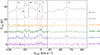 |
Fig. 2. Left: spectra of H I, CO, OH 1612, OH 1665, OH 1667, and OH 1720 MHz (from top to bottom) toward the H I arc. The x-axis and y-axis denote the velocity in km s−1 and the brightness temperature, respectively. Black dotted lines and velocity labels denote each of the velocity components in km s−1 as seen in the OH 1667 MHz emission. The scaling factor of each spectrum is listed in the right panel of this figure. To avoid overlapping, the spectra of H I, CO, and OH have been shifted upwards by multiples of 5 K on the y-axis. Right: same as in the left panel but showing a zoom onto the spectra at the −74 km s−1 component. |
As can be seen, each CO velocity component has a corresponding OH 1667 MHz component. However, the reverse is not always true. OH 1667 MHz emission (Tmb = 5.4 ± 1.4 mK, ΔV = 3.2 ± 0.9 km s−1) at −74 km s−1 is detected without any CO emission at the 3σ level. The particular −74 km s−1 velocity component is associated with the H I arc structure, confirming the existence of DMG therein. Furthermore, a weak absorption signature at the same velocity peak as OH is identified, which is considered to be the HINSA feature originally defined in the work of Li & Goldsmith (2003).
3.2. Column densities
3.2.1. H I
Assuming the H I 21 cm emission is optically thin, the column density of H I can be written as (Draine 2011):
![$$ \begin{aligned} N_{\rm HI} = 1.823 \times 10^{18} \int T_{\rm b}(\upsilon ) \mathrm{d}\upsilon (\mathrm{km\,s^{-1}}) \ [\mathrm{cm^{-2}}]. \end{aligned} $$](/articles/aa/full_html/2024/05/aa50067-24/aa50067-24-eq1.gif)
The column density of H I is calculated by integrating the recovered H I profile (Tb(υ)) with the same velocity range as the OH emission (−77 to −71 km s−1), resulting in a value of 2.4 × 1020 cm−2. As the H I profile has a much larger line width, the above value may be underestimated. Comparing with the result from Gaussian decomposition (see Appendix A), we include a 50% uncertainty on the H I column density.
3.2.2. OH
The column density of OH can be written as (Knapp & Kerr 1973; Dickey et al. 1981; Liszt & Lucas 1996):
![$$ \begin{aligned} N_{\rm OH} = 2.24 \times 10^{14} \frac{T_{\rm ex}}{T_{\rm ex}-T_{\rm bg}} \int T_{1667} \mathrm{d}\upsilon (\mathrm{km\,s^{-1}}) \ [\mathrm{cm^{-2}}], \end{aligned} $$](/articles/aa/full_html/2024/05/aa50067-24/aa50067-24-eq2.gif)
where Tex is the excitation temperature, Tbg is the cosmic microwave background (CMB) and synchrotron emission, and T1667 is the brightness temperature of OH 1667 MHz emission. The Tex of OH was first measured from absorption against quasars, and was found to be in the range of 4−8 K (Dickey et al. 1981). Liszt & Lucas (1996) measured OH 18 cm lines through both emission and absorption profiles toward eight quasars, in which they obtained Tex ≈ 3−5 K. Recent work by Li et al. (2018) found that the majority (∼90%) of OH components have Tex − Tbg ≲ 2 K. In our calculation, we adopt the value of Tex − Tbg = 1 K2. The resultant column density of OH is (2.0 ± 0.7) × 1013 cm−2.
3.3. HINSA
The key to obtaining the optical depth of HINSA absorption is to recover the background spectrum without the HINSA feature (Tb(υ)). The modeling of the HINSA profile follows the procedures of Krčo et al. (2008), in which we use the OH emission to set constraints on the central velocity (υ0) and the velocity dispersion (σ) of HINSA. A more detailed description of the procedures is discussed in Appendix B.
Figure 3 shows the recovered Tb(υ) (red dash line) and the optical depth profile of HINSA (green dotted line). The resultant central velocity is −74.1 km s−1, the full width at half maximum (FWHM) line width of HINSA is 1.53 km s−1, and the optical depth of HINSA is 0.084, corresponding to a HINSA column density of 3.8 × 1018 cm−2. The uncertainty in the fitting procedures is ∼19% (see Appendix B).
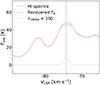 |
Fig. 3. Observed spectra of H I (black solid line), recovered Tb(υ) (red dash line), and the fitted optical depth of HINSA (green dotted line). The black vertical line represents the line velocity of HINSA. |
3.4. Molecular fraction of H I arc
We used the 3D E(B − V) map from Green et al. (2019) to obtain the total H-nucleus column density (NH), in which the 3D E(B − V) map is derived by combining high-quality stellar photometry from Pan-STARRS, 2MASS, and parallaxes from Gaia. The distance of H I Arc (5.6 ± 0.4 kpc from the Sun) is estimated from the latest rotational curve by Reid et al. (2019). The derived E(B − V) is 0.061 mag. Assuming AV/E(B − V) = 3.1 (Fitzpatrick 1999), this corresponds to AV = 0.19 mag.
Observations from diffuse X-ray absorption and emission and Lyα absorption have shown a linear relation between the total gas column density and interstellar reddening (NH/E(B − V) = 5.8 × 1021 cm−2 mag−1, Reina & Tarenghi 1973; Bohlin et al. 1978; Predehl & Schmitt 1995). However, recent studies found the conversion factor to be 1.5 times higher in diffuse lines of sight (e.g., 0.015 ≤ E(B − V) ≤ 0.075 mag) than the canonical value (Liszt 2014; Lenz et al. 2017; Nguyen et al. 2018). As our target includes diffuse lines of sight, we adopt the value of (9.4 ± 1.6) × 1021 cm−2 mag−1 (Nguyen et al. 2018). The resultant column density of H2 is NH2 = (NH − NHI)/2 = (1.7 ± 0.8) × 1020 cm−2. On the other hand, if we assume that the abundance of OH is in the order of 10−7 (Liszt & Lucas 1996; Nguyen et al. 2018; Li et al. 2018), we obtain a consistent H2 column density (NH2 = (2.0 ± 0.7)×1020 cm−2), as above. The inferred column density of H2 is therefore over an order of magnitude higher than the previous estimate (< 1019 cm−2, Knee & Brunt 2001).
The molecular gas fraction is given by fmol = 2NH2/NH = 59% ± 28%, which is similar to that of nearby diffuse clouds (∼20 − 44%, Luo et al. 2020). Our results suggest that a large fraction of molecular gas in the outer disk region of the Milky Way may be missing in the current CO surveys.
3.5. Abundances of CO and OH
The calculated abundance of OH with respect to H2 is (1.2 ± 0.7) × 10−7, which is similar to the median value in nearby diffuse and translucent cloud (1 × 10⁻⁷, Liszt & Lucas 1996, 2002; Weselak et al. 2010; Nguyen et al. 2018; Li et al. 2018; Luo et al. 2023a). The upper limit of CO abundance is 5 × 10⁻⁷ (3σ, see Appendix C), which is over two orders of magnitude lower than nearby molecular clouds (e.g., ∼8 − 10 × 10−5 in Taurus; Frerking et al. 1982; Goldsmith et al. 2008). This is consistent with high-sensitivity absorption measurements indicating that CO was only detected at regions for AV ≥ 0.32 mag and that the abundance of CO in diffuse clouds ranges from 2 × 10⁻⁷ to 5 × 10⁻⁶ (Luo et al. 2020).
4. Discussion
4.1. The fraction of HINSA and gas volume density
HINSA represents the H I gas that resides in the interior of the molecular cloud, which is produced by the cosmic ray (CR)-induced dissociation of H2. Thus, in chemical equilibrium, the steady-state HINSA density mainly depends on the CR ionization rate (ζ2), which is given by Goldsmith & Li (2005):

where k′ = 4 × 10⁻¹⁷ cm3 s−1 is the H2 formation rate coefficient (Gry et al. 2002). Assuming that ζ2 decreases exponentially with the increasing RGC (Wolfire et al. 2003), we adopt a value of 1.6 × 10⁻¹⁶ s−1, which is five times smaller than in nearby diffuse clouds of similar extinction (Luo et al. 2023b). Thus, the steady-state density of H I is nHI = 2.0 cm−3.
The fractional abundance of HINSA (NHINSA/NH2) in DMG is 0.022 ± 0.011, which is over an order of magnitude higher than that in nearby clouds (10−3, Li & Goldsmith 2003; Krčo & Goldsmith 2010; Tang et al. 2021), but is similar to the value in the early evolutionary stage of dark molecular clouds (0.02, Zuo et al. 2018). The inferred molecular gas density at steady state is nH2 = 91 ± 46 cm−3, which is similar to the measured density in nearby diffuse clouds (Luo et al. 2020, 2023b).
4.2. The formation mechanism of the DMG in the H I arc
The shell-like structure is a common feature in both Milky Way and external galaxies (Heiles 1979; Tenorio-Tagle & Bodenheimer 1988; Hatzidimitriou et al. 2005; Ehlerová & Palouš 2005, 2016; Dawson et al. 2013). The enormous H I supershells can be driven by the powerful stellar wind and radiation from massive stars and star clusters, and supernova explosions (McCray & Kafatos 1987; Elmegreen 1998; Seifried et al. 2020). In the solar neighborhood, giant molecular clouds are found to be at the surface of the Local Bubble, which is thought to have been induced by a supernova explosion ∼14 Myr ago (Zucker et al. 2022).
The existence of DMG in the cold H I arc structure and the corresponding large H I supershell GSH139-03-69 suggests a plausible scenario in which the formation of molecular gas is triggered by the expansion of the supershell. The expansion of the supershell generates powerful shockwaves that sweep up and compress the surrounding low-density ISM, leading to an enhancement of gas density as well as gravitational instability (Woodward 1976; Bisnovatyi-Kogan & Silich 1995; Elmegreen 1998; Wünsch et al. 2010).
The crossing timescale over which the shock waves pass through the H I arc is on the order of 107 yr (assuming a typical shock velocity of 10 km s−1, McCray & Kafatos 1987; Inutsuka et al. 2015). This timescale is much longer than the lifetime of giant molecular clouds (a few million years) and is also longer than the timescale required for H I to be converted into H2 (tHI − to − H2 = 1/(2k′nHI + ζ2)≈106 yr), enabling the formation of molecular gas during the expansion of the H I supershell. However, the low gas density and extinction may still be insufficient to build up the abundance of CO (Inutsuka et al. 2015; Seifried et al. 2020), which causes the H I arc to be dominated by DMG. Also, because the timescale on which the shell collapses to trigger star formation is inversely proportional to the midplane density (Elmegreen et al. 2002), supershell-driven cloud and star formation of this kind could be more frequent in the outer regions than in the nuclear regions of the galaxy. Our photodissociation regions (PDR) simulations suggest a cloud density of between 102 and 102.5 cm−3 and an evolution timescale of between 105 and 106 yr, which is consistent with the above analysis (see Appendix D).
For a rough estimate, assuming the cloud has a typical scale of a few to tens of parsecs, the DMG mass is on the order of 104 − 105 M⊙. Given the large number of supershells identified in the anticenter direction (a total number of 566; Suad et al. 2014), the DMG mass that is associated with the supershells could be on the order of 107 − 108 M⊙. This is of the same order of magnitude as the estimation of CO-dark diffuse molecular mass in the outer Galaxy (Busch et al. 2021) and the total mass traced by CO in the outer Galaxy (∼108 M⊙, Heyer & Dame 2015), suggesting that half of the molecular mass could be missed in CO surveys.
5. Conclusion
We confirm the existence of DMG toward a cold H I arc. This structure is not supposed to exist according to the canonical phased ISM models. The analysis from H I and OH spectra suggests an early evolution stage (t ≲ 106 yr) of low-density DMG. Our main conclusions are as follows:
-
We detect OH emission and the signature of HINSA toward the cold H I arc, where no CO emission is found. The existence of DMG associated with the H I arc supports the scenario that the expansion of the H I supershell triggers the formation of the molecular cloud.
-
The inferred H2 column density (1.7 ± 0.8 × 1020 cm−2) is over an order of magnitude higher than the previous estimate. The resultant fractional abundance of HINSA is 0.022 ± 0.011, which is an order of magnitude higher than that of nearby evolved clouds, but is similar to the values in the early evolutionary stage of dark clouds.
-
The derived column density of OH is (2.0 ± 0.7) × 1013 cm−2, and the resultant abundance is 1.2 ± 0.7 × 10⁻⁷. The upper limit of CO abundance is 5 × 10⁻⁷, which is more than an order of magnitude lower than that in nearby clouds.
-
The visual extinction (AV = 0.19 ± 0.03 mag), the inferred molecular fraction (59% ± 28%), and the gas density (nH2 = 91 ± 46 cm−3) of the DMG are similar to those of nearby diffuse clouds, suggesting similar properties of the CO-dark gas between the local and outer disk.
In addition, our findings show that the distribution of molecular gas in the outer disk regions could be much more extended than the gas traced by CO. This is consistent with previous high-sensitivity OH observations, where a diffuse thick DMG disk is traced by weak extended OH emission in the outer Galaxy (Busch et al. 2021). Future large OH surveys and an array covering the OH lines on FAST would improve our understanding of DMG in the outer Galaxy.
We revise the distance to 13 kpc according to the latest rotational curve by Reid et al. (2019).
Acknowledgments
We are grateful to the referee for the insightful review of our manuscript, which improved the quality and clarity of our work. We thank the scientific staff and telescope operators at the Green Bank Observatory (GBO) for their advice and assistance with the remote observations, in particular Tapasi Ghosh, and for the support of the data reduction, especially Pedro Salas. This work has been supported by the National Natural Science Foundation of China (grant No. 12041305,12173016), Cultivation Project for FAST scientific Payoff and Research achievement of CAMS-CAS, China Postdoctoral Science Foundation (grant No. 2021M691533), the Program for Innovative Talents, Entrepreneur in Jiangsu, the science research grants from the China Manned Space Project with NO.CMS-CSST-2021-A08. N.Y.T. acknowledges support from the University Annual Scientific Research Plan of Anhui Province (No. 2023AH030052, No. 2022AH010013), Zhejiang Lab Open Research Project (No. K2022PE0AB01), Cultivation Project for FAST Scientific Payoff and Research Achievement of CAMS-CAS. The Green Bank Observatory is a facility of the National Science Foundation operated under cooperative agreement by Associated Universities, Inc. The Canadian Galactic Plane Survey (CGPS) is a Canadian project with international partners. The Dominion Radio Astrophysical Observatory is operated as a national facility by the National Research Council of Canada. The Five College Radio Astronomy Observatory CO Survey of the Outer Galaxy was supported by NSF grant AST 94-20159. The CGPS is supported by a grant from the Natural Sciences and Engineering Research Council of Canada.
References
- Bisbas, T. G., Bell, T. A., Viti, S., Yates, J., & Barlow, M. J. 2012, MNRAS, 427, 2100 [NASA ADS] [CrossRef] [Google Scholar]
- Bisbas, T. G., Schruba, A., & van Dishoeck, E. F. 2019, MNRAS, 485, 3097 [NASA ADS] [Google Scholar]
- Bisnovatyi-Kogan, G. S., & Silich, S. A. 1995, Rev. Mod. Phys., 67, 661 [Google Scholar]
- Bohlin, R. C., Savage, B. D., & Drake, J. F. 1978, ApJ, 224, 132 [Google Scholar]
- Bolatto, A. D., Wolfire, M., & Leroy, A. K. 2013, ARA&A, 51, 207 [CrossRef] [Google Scholar]
- Busch, M. P., Engelke, P. D., Allen, R. J., & Hogg, D. E. 2021, ApJ, 914, 72 [CrossRef] [Google Scholar]
- Dame, T. M., Hartmann, D., & Thaddeus, P. 2001, ApJ, 547, 792 [Google Scholar]
- Dawson, J. R., McClure-Griffiths, N. M., Wong, T., et al. 2013, ApJ, 763, 56 [NASA ADS] [CrossRef] [Google Scholar]
- Dickey, J. M., & Lockman, F. J. 1990, ARA&A, 28, 215 [Google Scholar]
- Dickey, J. M., Crovisier, J., & Kazes, I. 1981, A&A, 98, 271 [NASA ADS] [Google Scholar]
- Draine, B. T. 1978, ApJS, 36, 595 [Google Scholar]
- Draine, B. T. 2011, Physics of the Interstellar and Intergalactic Medium (Princeton: Princeton University Press) [Google Scholar]
- Ehlerová, S., & Palouš, J. 2005, A&A, 437, 101 [NASA ADS] [CrossRef] [EDP Sciences] [Google Scholar]
- Ehlerová, S., & Palouš, J. 2016, A&A, 587, A5 [NASA ADS] [CrossRef] [EDP Sciences] [Google Scholar]
- Elmegreen, B. G. 1998, in Origins, eds. C. E. Woodward, J. M. Shull, J. Thronson, & A. Harley, ASP Conf. Ser., 148, 150 [NASA ADS] [Google Scholar]
- Elmegreen, B. G., Palouš, J., & Ehlerová, S. 2002, MNRAS, 334, 693 [NASA ADS] [CrossRef] [Google Scholar]
- Federman, S. R., Weber, J., & Lambert, D. L. 1996, ApJ, 463, 181 [NASA ADS] [CrossRef] [Google Scholar]
- Field, G. B., Goldsmith, D. W., & Habing, H. J. 1969, ApJ, 155, L149 [NASA ADS] [CrossRef] [Google Scholar]
- Fitzpatrick, E. L. 1999, PASP, 111, 63 [Google Scholar]
- Frerking, M. A., Langer, W. D., & Wilson, R. W. 1982, ApJ, 262, 590 [Google Scholar]
- Goldsmith, P. F. 2013, ApJ, 774, 134 [NASA ADS] [CrossRef] [Google Scholar]
- Goldsmith, P. F., & Li, D. 2005, ApJ, 622, 938 [NASA ADS] [CrossRef] [Google Scholar]
- Goldsmith, P. F., Heyer, M., Narayanan, G., et al. 2008, ApJ, 680, 428 [Google Scholar]
- Green, G. M., Schlafly, E., Zucker, C., Speagle, J. S., & Finkbeiner, D. 2019, ApJ, 887, 93 [NASA ADS] [CrossRef] [Google Scholar]
- Grenier, I. A., Casandjian, J.-M., & Terrier, R. 2005, Science, 307, 1292 [Google Scholar]
- Gry, C., Boulanger, F., Nehmé, C., et al. 2002, A&A, 391, 675 [NASA ADS] [CrossRef] [EDP Sciences] [Google Scholar]
- Haslam, C. G. T., Salter, C. J., Stoffel, H., & Wilson, W. E. 1982, A&AS, 47, 1 [NASA ADS] [Google Scholar]
- Hatzidimitriou, D., Stanimirovic, S., Maragoudaki, F., et al. 2005, MNRAS, 360, 1171 [NASA ADS] [CrossRef] [Google Scholar]
- Heiles, C. 1979, ApJ, 229, 533 [NASA ADS] [CrossRef] [Google Scholar]
- Heiles, C., & Troland, T. H. 2003, ApJ, 586, 1067 [NASA ADS] [CrossRef] [Google Scholar]
- Heyer, M., & Dame, T. M. 2015, ARA&A, 53, 583 [Google Scholar]
- Heyer, M. H., Brunt, C., Snell, R. L., et al. 1998, ApJS, 115, 241 [NASA ADS] [CrossRef] [Google Scholar]
- Hu, C.-Y., Sternberg, A., & van Dishoeck, E. F. 2021, ApJ, 920, 44 [NASA ADS] [CrossRef] [Google Scholar]
- Inutsuka, S.-I., Inoue, T., Iwasaki, K., & Hosokawa, T. 2015, A&A, 580, A49 [NASA ADS] [CrossRef] [EDP Sciences] [Google Scholar]
- Kalberla, P. M. W., & Kerp, J. 2009, ARA&A, 47, 27 [NASA ADS] [CrossRef] [Google Scholar]
- Knapp, G. R., & Kerr, F. J. 1973, AJ, 78, 453 [NASA ADS] [CrossRef] [Google Scholar]
- Knee, L. B. G., & Brunt, C. M. 2001, Nature, 412, 308 [CrossRef] [Google Scholar]
- Krčo, M., & Goldsmith, P. F. 2010, ApJ, 724, 1402 [CrossRef] [Google Scholar]
- Krčo, M., Goldsmith, P. F., Brown, R. L., & Li, D. 2008, ApJ, 689, 276 [CrossRef] [Google Scholar]
- Lee, M.-Y., Stanimirović, S., Murray, C. E., Heiles, C., & Miller, J. 2015, ApJ, 809, 56 [NASA ADS] [CrossRef] [Google Scholar]
- Lenz, D., Hensley, B. S., & Doré, O. 2017, ApJ, 846, 38 [NASA ADS] [CrossRef] [Google Scholar]
- Li, D., & Goldsmith, P. F. 2003, ApJ, 585, 823 [NASA ADS] [CrossRef] [Google Scholar]
- Li, D., Tang, N., Nguyen, H., et al. 2018, ApJS, 235, 1 [Google Scholar]
- Liszt, H. 2014, ApJ, 780, 10 [Google Scholar]
- Liszt, H., & Lucas, R. 1996, A&A, 314, 917 [Google Scholar]
- Liszt, H., & Lucas, R. 2002, A&A, 391, 693 [NASA ADS] [CrossRef] [EDP Sciences] [Google Scholar]
- Luo, G., Li, D., Tang, N., et al. 2020, ApJ, 889, L4 [NASA ADS] [CrossRef] [Google Scholar]
- Luo, G., Zhang, Z.-Y., Bisbas, T. G., et al. 2023a, ApJ, 942, 101 [NASA ADS] [CrossRef] [Google Scholar]
- Luo, G., Zhang, Z.-Y., Bisbas, T. G., et al. 2023b, ApJ, 946, 91 [NASA ADS] [CrossRef] [Google Scholar]
- Mangum, J. G., & Shirley, Y. L. 2015, PASP, 127, 266 [Google Scholar]
- McCray, R., & Kafatos, M. 1987, ApJ, 317, 190 [NASA ADS] [CrossRef] [Google Scholar]
- McElroy, D., Walsh, C., Markwick, A. J., et al. 2013, A&A, 550, A36 [NASA ADS] [CrossRef] [EDP Sciences] [Google Scholar]
- McKee, C. F., & Ostriker, J. P. 1977, ApJ, 218, 148 [NASA ADS] [CrossRef] [Google Scholar]
- Méndez-Delgado, J. E., Amayo, A., Arellano-Córdova, K. Z., et al. 2022, MNRAS, 510, 4436 [CrossRef] [Google Scholar]
- Nguyen, H., Dawson, J. R., Miville-Deschênes, M. A., et al. 2018, ApJ, 862, 49 [NASA ADS] [CrossRef] [Google Scholar]
- Pineda, J. L., Langer, W. D., Velusamy, T., & Goldsmith, P. F. 2013, A&A, 554, A103 [CrossRef] [EDP Sciences] [Google Scholar]
- Planck Collaboration XIX. 2011, A&A, 536, A19 [NASA ADS] [CrossRef] [EDP Sciences] [Google Scholar]
- Predehl, P., & Schmitt, J. H. M. M. 1995, A&A, 500, 459 [Google Scholar]
- Reid, M. J., Menten, K. M., Brunthaler, A., et al. 2019, ApJ, 885, 131 [Google Scholar]
- Reina, C., & Tarenghi, M. 1973, A&A, 26, 257 [NASA ADS] [Google Scholar]
- Remy, Q., Grenier, I. A., Marshall, D. J., & Casandjian, J. M. 2017, A&A, 601, A78 [NASA ADS] [CrossRef] [EDP Sciences] [Google Scholar]
- Rybarczyk, D. R., Stanimirović, S., Gong, M., et al. 2022, ApJ, 928, 79 [NASA ADS] [CrossRef] [Google Scholar]
- Sahai, R., & Nyman, L.-Å. 1997, ApJ, 487, L155 [NASA ADS] [CrossRef] [Google Scholar]
- Sahai, R., Vlemmings, W. H. T., Huggins, P. J., Nyman, L. Å., & Gonidakis, I. 2013, ApJ, 777, 92 [NASA ADS] [CrossRef] [Google Scholar]
- Seifried, D., Haid, S., Walch, S., Borchert, E. M. A., & Bisbas, T. G. 2020, MNRAS, 492, 1465 [NASA ADS] [CrossRef] [Google Scholar]
- Suad, L. A., Caiafa, C. F., Arnal, E. M., & Cichowolski, S. 2014, A&A, 564, A116 [NASA ADS] [CrossRef] [EDP Sciences] [Google Scholar]
- Tang, N., Li, D., Yue, N., et al. 2021, ApJS, 252, 1 [Google Scholar]
- Tang, N.-Y., Zuo, P., Li, D., et al. 2020, Res. Astron. Astrophys., 20, 077 [CrossRef] [Google Scholar]
- Taylor, A. R., Gibson, S. J., Peracaula, M., et al. 2003, AJ, 125, 3145 [NASA ADS] [CrossRef] [Google Scholar]
- Tenorio-Tagle, G., & Bodenheimer, P. 1988, ARA&A, 26, 145 [NASA ADS] [CrossRef] [Google Scholar]
- Weselak, T., Galazutdinov, G. A., Beletsky, Y., & Krełowski, J. 2010, MNRAS, 402, 1991 [NASA ADS] [CrossRef] [Google Scholar]
- Wilson, R. W., Jefferts, K. B., & Penzias, A. A. 1970, ApJ, 161, L43 [NASA ADS] [CrossRef] [Google Scholar]
- Wolfire, M. G., McKee, C. F., Hollenbach, D., & Tielens, A. G. G. M. 2003, ApJ, 587, 278 [Google Scholar]
- Woodward, P. R. 1976, ApJ, 207, 484 [NASA ADS] [CrossRef] [Google Scholar]
- Wünsch, R., Dale, J. E., Palouš, J., & Whitworth, A. P. 2010, MNRAS, 407, 1963 [CrossRef] [Google Scholar]
- Zucker, C., Goodman, A. A., Alves, J., et al. 2022, Nature, 601, 334 [NASA ADS] [CrossRef] [Google Scholar]
- Zuo, P., Li, D., Peek, J. E. G., et al. 2018, ApJ, 867, 13 [NASA ADS] [CrossRef] [Google Scholar]
Appendix A: Gaussian decomposition of H I
The H I profile usually exhibits a larger line width than the molecular line counterpart. To evaluate the uncertainties in deriving the H I column density in Section 3.2.1, we performed Gaussian decomposition of the H I profile. Figure A.1 shows the Gaussian decomposition of the recovered Tb(υ) profiles and the residual after the fitting. The Gaussian fitting result at −74.1 km s−1 has a brightness temperature of 35±1 K and a line width of 5.5±0.1 km s−1. The H I column density calculated from equation 1 is (3.7±0.1)×1020 cm−2, which is 50% higher than the value in Section 3.2.1. Thus, we consider that there is an overall 50% uncertainty on the H I column density.
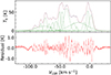 |
Fig. A.1. Gaussian decomposition of the recovered Tb(υ) (upper panel) and the residual after the fitting (lower panel). |
Appendix B: modeling of the HINSA profile
Considering the three-component H I model, the observed H I profile (TR) is a combination of background emission, cold H I absorption against the background, and foreground emission between the cold H I and the observer. Assuming that the atomic cloud has a uniform temperature and small optical depth, following equation (8) in Li & Goldsmith (2003), the radiative transfer equation of the modeled background spectrum can be written as:
where TR is the observed spectrum; Tc is the background continuum, which includes the cosmic microwave background (CMB, 2.73 K) and the Galactic synchrotron background; Tk is the excitation temperature of the cold H I, which is equal to the kinetic temperature of molecular gas (here we take a typical kinetic temperature of 15 K); τf and τ(υ) are the optical depth of the foreground H I gas and HINSA, respectively; p is the fraction of the H I in the background, which is defined as p = τb/τtot; τf is assumed as 0.1 in our calculation, which would only result in < 3% uncertainty on the optical depth of HINSA as long as the optically thin assumption is valid; and Tc is estimated from the 408 MHz all-sky continuum survey through the equation: Tc = TCMB + T408(ν/408)−2.8 (Haslam et al. 1982). The continuum emission in our target region is 60 K at 408 MHz, resulting in a Tc of 4.6 K.
Following equation (9) in Li & Goldsmith (2003), p can be estimated from the geometry of the galactic disk:
![$$ \begin{aligned} p = \mathrm{erfc}\left[\frac{\sqrt{4 ln2} D sin(b)}{z}\right], \end{aligned} $$](/articles/aa/full_html/2024/05/aa50067-24/aa50067-24-eq5.gif)
where D is the distance of the cloud, b is the Galactic latitude, and z is the scale height. With the full consideration of H I density distribution, the kinematic distance, and the scale height at the cloud position. In our calculations, we take a p value of ∼0.9. We stress here that the p value should not be much less than 1; otherwise, the HINSA signature would be obscured by the foreground emission (Krčo et al. 2008).
To recover the background spectrum without HINSA, we follow the procedures in Krčo et al. (2008). The optical depth of HINSA (τ(υ)) can be described as a Gaussian function:
where τ0 is the peak of optical depth, υ0 is the central velocity, and σ is the velocity dispersion of HINSA. We used the OH emission to set constraints on the central velocity (υ0) and velocity dispersion (σ) of HINSA.
As the second derivative of a Gaussian function is sensitive to the velocity dispersion, and the velocity dispersion of HINSA (∼1 km s−1) is much narrower than that of background H I (> 5 km s−1), the second derivative of H I profile usually have large jumps at the velocity range of HINSA, even when the HINSA is relatively weak (Krčo et al. 2008). Thus, minimizing the integration of the second derivative of the recovered background spectrum (Tb(υ)), we would simultaneously obtain the reasonable parameters (τ0, υ0, and σ) (Krčo et al. 2008).
From our fitting procedure, varying the p value to 0.8≤p≤1 and the assumption of Tk from 10 to 25 K would result in an uncertainty on τ(υ) of within 19%. Varying τf would not bring too many uncertainties (≲10% even if τf ∼ 1), but would increase the upper limit of Tk (up to 35 K) required to produce HINSA. Thus, we consider an overall uncertainty on τ(υ) of 19%. This is far below the uncertainty from the polynomial fitting procedures (∼50%, Li & Goldsmith 2003).
Appendix C: The 3σ upper limit of CO
The column density can be written as a function of optical depth (τν, Mangum & Shirley 2015):
where |μlu|2 is the dipole matrix element, Qrot is the rotational partition function, gu is the degeneracy of upper energy level, Eu is the upper energy level, and Tex is the excitation temperature. According to the radiative transfer equation, the main beam brightness temperature Tmb is given by the expression,
, \end{aligned} $$](/articles/aa/full_html/2024/05/aa50067-24/aa50067-24-eq8.gif)
where ηmb is the main beam efficiency, and fb is the beam filling factor (assumed to be 1 in the following calculation). Tbg is the background continuum, which should be equal to the 2.73 K for CO, and 3.9 K for OH 1667 MHz including the Galactic synchrotron background. The temperature terms in equation C.2 is in the form of the Planck function: J(T) = (hν/k)/(exp(hν/kT)−1) at millimeter wavelengths.
With the optically thin assumption (τν ≪ 1), equation C.1 can be rewritten in the form of Tb:
For each transition, the |μlu|2, Eu, and rest frequency ν are taken from SPLATALOGUE3.
We adopt a typical value measured from diffuse clouds, which is Tex = 4 K (Goldsmith 2013; Luo et al. 2020). If we fill in all the constants in equation C.3, a convenient form of this equation is:
![$$ \begin{aligned} \begin{aligned} N_{\rm CO} =&6.61 \times 10^{14} Q_{\rm rot}e^{\frac{5.53}{T_{\mathrm{ex}}}} \left[e^{\frac{5.53}{T_{\mathrm{ex}}}}-1 \right]^{-1} \\&\frac{\int T_{\mathrm{mb}} d\upsilon (\mathrm{km\,s^{-1}})}{J(T_{\mathrm{ex}})-0.84} \ [\mathrm{cm^{-2}}]. \end{aligned} \end{aligned} $$](/articles/aa/full_html/2024/05/aa50067-24/aa50067-24-eq10.gif)
The line rms of CO within 0.5° regions is 5.5 mK, and therefore the resultant 3σ upper limit of CO column density is 9 × 1013 cm−2.
Appendix D: PDR modeling
We used the publicly available PDR code4 3D-PDR (Bisbas et al. 2012) to model the gas properties of the H I arc. 3D-DPR models one- and three-dimensional density distributions; it calculates the attenuation of the FUV radiation field in every depth point and outputs the self-consistent solutions of chemical abundances, gas and dust temperature, emissivities, and level populations by performing iterations over thermal balance (see Bisbas et al. 2012 for more description). In the 3D-PDR models, we used a reduced network, which contains 33 species and 330 reactions taken from the UMIST2012 network (McElroy et al. 2013). The initial gas phase abundances of He, C+, and O are 9 × 10⁻², 1.5 × 10⁻⁴ and 3 × 10⁻⁴, respectively.
Figure D.1 shows the results under gas volume density nH = 102, 102.5, and 103 cm−3, and evolution timescale t = 105, 105.5, and 106 yr. The external UV radiation field is taken as χ/χ0 = 0.3 (normalized to the spectral shape of Draine 1978), assuming an exponential decrease as a function of RGC (Wolfire et al. 2003). The cosmic-ray ionization rate is taken as 1.6 × 10⁻¹⁶ s−1 (Section 4.1). The metallicity is scaled with RGC and taken to be 1/2 Z⊙ (Méndez-Delgado et al. 2022). The column densities from the models are integrated along the line of sight. The observational results favor the models with a gas density in the range of 102 ≤ nH ≤ 102.5 cm−3 and an evolution timescale in the range of 105 ≤ t ≤ 106 yr, which is consistent with our analysis in Section 4.1. This dependency on the evolution timescale was also recently addressed by Hu et al. (2021).
 |
Fig. D.1. Modeling results of NHI, NOH, and NCO under different physical parameters (from left to right, respectively). The orange, green, and blue curves represent the evolution timescale t = 105, 105.5, and 106 yr. The solid, dashed, and dotted curves represent the gas densities nH = 102, 102.5, and 103 cm−3. The black points denote data from observations. |
The predicted CO column density is lower than the detection limit by a factor of 2∼5. Given that the gas traced by CO may have a beam filling factor of fb < 1, the detection limit should be higher. On the other hand, the formation of CO in our models does not consider the enhancement due to the neutral–ion reactions through the propagation of Alfvén waves (Federman et al. 1996). Such an enhancement would result in an increase in the CO column density at low AV (AV < 1.5 mag for nH = 102 cm−3, Bisbas et al. 2019) by up to an order of magnitude.
All Figures
|
Fig. 1. H I integrated intensity (background gray scale) from the Canadian Galactic Plane Survey (CGPS, Taylor et al. 2003) and CO integrated intensity (green contours, 0.4 K km s−1 × (3, 5, 10)) from the Outer Galaxy Survey (OGS, Heyer et al. 1998). The integrated velocity range is −80 to −73 km s−1 for both H I and CO. The H I arc is denoted by the red curves. The yellow square denotes the position where the inferred H I spin temperature is ∼10 K in Knee & Brunt (2001). The blue cross denotes the H I pointing observations, and the blue square is the region mapped in OH. |
| In the text | |
|
Fig. 2. Left: spectra of H I, CO, OH 1612, OH 1665, OH 1667, and OH 1720 MHz (from top to bottom) toward the H I arc. The x-axis and y-axis denote the velocity in km s−1 and the brightness temperature, respectively. Black dotted lines and velocity labels denote each of the velocity components in km s−1 as seen in the OH 1667 MHz emission. The scaling factor of each spectrum is listed in the right panel of this figure. To avoid overlapping, the spectra of H I, CO, and OH have been shifted upwards by multiples of 5 K on the y-axis. Right: same as in the left panel but showing a zoom onto the spectra at the −74 km s−1 component. |
| In the text | |
|
Fig. 3. Observed spectra of H I (black solid line), recovered Tb(υ) (red dash line), and the fitted optical depth of HINSA (green dotted line). The black vertical line represents the line velocity of HINSA. |
| In the text | |
|
Fig. A.1. Gaussian decomposition of the recovered Tb(υ) (upper panel) and the residual after the fitting (lower panel). |
| In the text | |
|
Fig. D.1. Modeling results of NHI, NOH, and NCO under different physical parameters (from left to right, respectively). The orange, green, and blue curves represent the evolution timescale t = 105, 105.5, and 106 yr. The solid, dashed, and dotted curves represent the gas densities nH = 102, 102.5, and 103 cm−3. The black points denote data from observations. |
| In the text | |
Current usage metrics show cumulative count of Article Views (full-text article views including HTML views, PDF and ePub downloads, according to the available data) and Abstracts Views on Vision4Press platform.
Data correspond to usage on the plateform after 2015. The current usage metrics is available 48-96 hours after online publication and is updated daily on week days.
Initial download of the metrics may take a while.