| Issue |
A&A
Volume 584, December 2015
|
|
|---|---|---|
| Article Number | A129 | |
| Number of page(s) | 21 | |
| Section | Astrophysical processes | |
| DOI | https://doi.org/10.1051/0004-6361/201527052 | |
| Published online | 08 December 2015 | |
Online material
Appendix A: Kalnajs basis
We now detail the properties of the basis introduced in Kalnajs (1976) to describe 2D discs5. The basis depends on two parameters: an index kKa ∈N and a scale radius rKa ∈ R+. In all the upcoming formulae of this section, in order to shorten the notations, we write r for the dimensionless quantity r/rKa. As introduced previously in Eq. (16), the basis elements depend on two indices: the azimuthal number ℓ and the radial index n. One should note that we have ℓ ≥ 0 and n ≥ 0. The radial component of the potential elements are then of the form 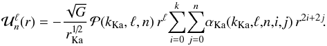 (A.1)The radial component of the density elements is given by
 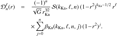 (A.2)In Eqs. (A.1) and (A.2), the coefficients
 ![]() and
and ![]() are defined by
are defined by 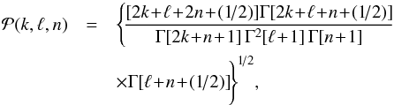 (A.3)and
 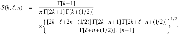 (A.4)Finally, in Eqs. (A.1) and (A.2), we have also introduced
 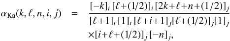 (A.5)and
 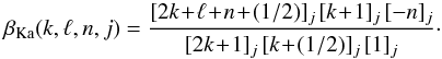 (A.6)In the two previous expressions, we introduced the rising Pochhammer symbol [ a ] i defined as
 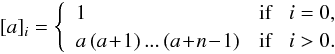 (A.7)
(A.7)
Appendix B: Calculation of ℵ
We now detail how the analytical function ℵ from Eq. (32) may be computed. In order to ease the implementation of its computation, we rewrite ℵ in an undimensionalised way as follows 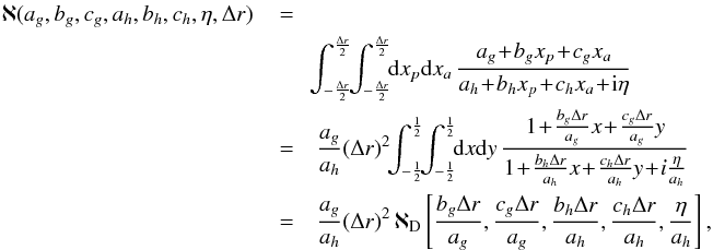 (B.1)where we assumed that ag,ah ≠ 0 and used the change of variables x = xp/ Δr and y = xa/ Δr. We also defined the dimensionless function ℵD as
  (B.2)To compute this integral, we may now exhibit a function G(x,y) such that
  (B.3)One possible choice for G is given by
  (B.4)One should note in the previous expression the presence of a complex logarithm and a tan-1. However, because e,f,η ∈R and η ≠ 0, one can easily show that the arguments of both of these functions never cross the usual branch-cut of these functions {Im(z) = 0; Re(z) ≤ 0 }. As a consequence, the expression (B.2) can immediately be computed as
 ![]() (B.5)
(B.5)
Appendix C: Response matrix and N-body validations
The computation of the response matrix as described in Sect. 3 was validated by recovering the results of the pioneer work of Zang (1976), extended in Evans & Read (1998a,b), and recovered numerically in Sellwood & Evans (2001). These papers predicted the precession rate ω0 = mφΩp and growth rate η = s of the unstable modes of a truncated Mestel disc similar to the stable one described in Sect. 4.1. To build up an unstable disc similar to the ones considered in these previous works, one has to consider a fully active disc, so that ξ = 1. So as to have Q = 1 (Toomre 1964), the velocity dispersion within the disc is given by q = 6, where the parameter q has been introduced in Eq. (46). Finally, a last parameter one can tune in order to modify the properties of the disc is the truncation index of the inner tapering νt defined in Eq. (48). While looking only for mφ = 2 modes, we considered three different truncations indices given by νt = 4, 6, 8. To compute the response matrix, we used the same numerical parameters as described in Sect. 4.2. Looking for unstable modes amounts to looking for complex frequencies ω = ω0 + iη such that the response matrix ![]() from Eq. (24) possesses an eigenvalue equal to 1. Such a complex frequency is then associated with an unstable mode of pattern speed ω0 and growth rate η. To determine the growth rate and pattern speed of the unstable modes, we relied on Nyquist contours similarly to the technique presented in Pichon & Cannon (1997). For a fixed value of η, one can study the continuous complex curve
from Eq. (24) possesses an eigenvalue equal to 1. Such a complex frequency is then associated with an unstable mode of pattern speed ω0 and growth rate η. To determine the growth rate and pattern speed of the unstable modes, we relied on Nyquist contours similarly to the technique presented in Pichon & Cannon (1997). For a fixed value of η, one can study the continuous complex curve ![]() . Because for η → + ∞, one has
. Because for η → + ∞, one has ![]() , the number of windings of this curve around the origin gives a lower bound on the number of unstable modes with a growth rate superior to η. By decreasing the value of η, one can then determine the largest value of η admitting an unstable mode, and therefore the most unstable mode of the disc. The Nyquist contours obtained for the truncation index νt = 6 are illustrated in Fig. C.1, while the measurements are gathered in Table C.1.
, the number of windings of this curve around the origin gives a lower bound on the number of unstable modes with a growth rate superior to η. By decreasing the value of η, one can then determine the largest value of η admitting an unstable mode, and therefore the most unstable mode of the disc. The Nyquist contours obtained for the truncation index νt = 6 are illustrated in Fig. C.1, while the measurements are gathered in Table C.1.
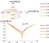 |
Fig. C.1
Top panel: zoomed Nyquist contours in the complex plane of |
| Open with DEXTER | |
Once the characteristics (ω0,η) of the unstable modes have been determined, one can study in the physical space the shape of the mode. Indeed, for ω = ω0 + iη, one can compute ![]() , and numerically diagonalise this matrix. One then considers its eigenvector Xmode (of size nmax, where nmax is the number of basis elements considered) associated with the eigenvalue almost equal to 1. The shape of the mode is then immediately given by
, and numerically diagonalise this matrix. One then considers its eigenvector Xmode (of size nmax, where nmax is the number of basis elements considered) associated with the eigenvalue almost equal to 1. The shape of the mode is then immediately given by  (C.1)where Σ(p) are the considered surface density basis elements. The shape of the recovered unstable mode for the truncated νt = 4 Mestel disc is illustrated in Fig. C.2.
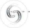 |
Fig. C.2
Unstable mode for the truncated νt = 4 Mestel disc recovered via the matrix method presented in Sect. 3. Only positive contour levels are shown and are spaced linearly between 10% and 90% of the maximum norm. The radii associated with the resonances ILR, COR and OLR have been represented, as given by ω0 = m·Ω(Rm), where the intrinsic frequencies Ω(R) = (Ωφ(R),κ(R)) have to be computed within the epicyclic approximation. For a Mestel disc, they are given by Ωφ(R) = V0/R and |
| Open with DEXTER | |
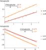 |
Fig. C.3
Measurement of the growth rate η and pattern speed ω0 of the mφ = 2 unstable modes of truncated Mestel discs with a random velocity given by q = 6 for various values of the truncation index νt = 6, 8. The basis coefficient plotted is associated with the basis element (ℓ,n) = (2,0), using the same basis elements as for the matrix method in Sect. 4.2. |
| Open with DEXTER | |
The same unstable modes were also used to validate the N-body code presented in Sect. 5. To run these simulations, we used the same sampling technique as described in Appendix E. In order not to be significantly impacted by the absence of a quiet start sampling (Sellwood 1983), for each value of νt, the measurements were performed with simulations of 20M particles. As observed in Sellwood & Evans (2001), the appropriate setting of the parameters of the N-body code are crucial to recover correctly the unstable modes of a disc. We considered a grid made with Nmesh = 120 grid cells, while using a softening length equal to ε = Ri/ 60. As described in Sect. 5, we similarly restricted the perturbing forces only to the harmonic sector mφ = 2, using Nring = 2400 radial rings, with Nφ = 720 azimuthal points. In order to extract the properties of the mode present within the disc, one may proceed as follows. For each simulation snapshot, one can estimate the active surface density within the disc via ![]() (C.2)where the sum on i is made on all the particles of the simulation and xi(t) is the position of the ith particle at time t. Such a surface density can be decomposed on the basis elements from Eq. (3) in the form
(C.2)where the sum on i is made on all the particles of the simulation and xi(t) is the position of the ith particle at time t. Such a surface density can be decomposed on the basis elements from Eq. (3) in the form  (C.3)where the sum on p is made on all the basis elements Σ(p) considered. The effective basis elements used during our measurements are the same as the ones used in the matrix method from Sect. 4.2. Thanks to the biorthogonality property from Eq. (3), the coefficients bp(t) can be immediately determined as
  (C.4)As we are looking for unstable modes within the disc, we expect to have bp(t) ∝ exp [ −i(ω0 + iη)t ], where ω0 = mφΩp is the pattern speed of the mode and η = s its growth rate. As a consequence, one immediately obtains that
 ![]() (C.5)if one is sufficently careful with the branch-cut of the complex logarithm. Such a linear scaling with t of Re(log (bp(t))) and Im(log (bp(t))) is therefeore the appropriate measurement procedure to use in order to estimate the growth rate and pattern speed of the unstable modes of these truncated Mestel discs. The measurements for the various values of the truncation index νt are illustrated in Fig. C.3. Once the basis coefficients bp(t) have been determined, one can study the shape of the recovered unstable modes in the physical space. Indeed, similarly to Eq. (C.1), the shape of the modes is given by
(C.5)if one is sufficently careful with the branch-cut of the complex logarithm. Such a linear scaling with t of Re(log (bp(t))) and Im(log (bp(t))) is therefeore the appropriate measurement procedure to use in order to estimate the growth rate and pattern speed of the unstable modes of these truncated Mestel discs. The measurements for the various values of the truncation index νt are illustrated in Fig. C.3. Once the basis coefficients bp(t) have been determined, one can study the shape of the recovered unstable modes in the physical space. Indeed, similarly to Eq. (C.1), the shape of the modes is given by 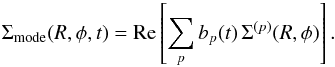 (C.6)In analogy with Fig. C.2, for which the unstable modes have been obtained via the matrix method, Fig. C.4 illustrates the unstable mode of the same truncated νt = 4 Mestel disc.
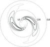 |
Fig. C.4
Unstable mode for the truncated νt = 4 Mestel disc recovered via direct N-body simulations as presented in Sect. 5. Only positive contour levels are shown and are spaced linearly between 20% and 80% of the maximum norm. Similarly to Fig. C.2, the radii associated with the resonances ILR, COR and OLR have been represented. |
| Open with DEXTER | |
Measurements of the pattern speed ω0 = mφΩp and growth rate η = s for unstable mφ = 2 modes of tapered Mestel discs.
As a conclusion, the growth rates and pattern speeds obtained either via the matrix method or direct N-body simulations are gathered in Table C.1. As observed in Sellwood & Evans (2001), the recovery of the unstable modes characteristics from direct N-body simulations when performed for truncated Mestel discs is a difficult task, for which convergence to the values predicted through linear theory may be difficult.
Appendix D: Why swing matters?
Let us investigate here briefly the importance of self-gravitation and the completeness of the projection basis in capturing the role of swing amplification.
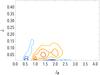 |
Fig. D.1
Map of |
| Open with DEXTER | |
Appendix D.1: Turning off the self-gravitating amplification
In order to investigate the role of the self-gravitating amplification, one may perform the same estimation as presented in Fig. 4, while neglecting collective effects. When neglecting collective effects, i.e. when assuming that ![]() , one recovers the inhomogeneous Landau equation (Chavanis 2013) which reads
, one recovers the inhomogeneous Landau equation (Chavanis 2013) which reads  (D.1)Equation (D.1) involves the bare susceptibility coefficients | Am1,m2(J1,J2) | 2, which can be equivalently defined (see Appendix B of Paper I) by
  (D.2)where u(x) is the binary potential of interaction given by u(x) = −G/| x | for gravity. This estimation therefore does not require to estimate the response matrix from Eq. (24), but one still has to perform integrations along the resonant lines as in Eq. (42). Let us provide a first numerical implementation of this equation in the context of galactic dynamics. The contours of
 ![]() are illustrated in Fig. D.1. Comparing the maps of the dressed diffusion flux Ndiv(ℱtot) from Fig. 4 and the bare diffusion flux
are illustrated in Fig. D.1. Comparing the maps of the dressed diffusion flux Ndiv(ℱtot) from Fig. 4 and the bare diffusion flux ![]() , allows us to assess the strength of the self-gravitating amplification. As expected, when turning off the self-gravity of the system, one reduces significantly the susceptibility of the system and therefore slows down its secular evolution by a factor of about 1000. One may also remark that while the secular appearance of a resonant ridge in the dressed diffusion from Fig. 4 was obvious, the shape of the contours obtained in the bare Fig. D.1 do not emphasise as clearly the appearance of such a narrow resonant ridge. One can still remark that the structure of the bare contours obtained in Fig. D.1 is similar to what was obtained in Fig. 9 of Paper I, through the WKB limit of the Balescu-Lenard equation. One can finally note that the amplitudes of the bare divergence contours obtained previously are similar to the WKB values obtained in Paper I. As a consequence, the comparison of Figs. 4 and D.1 emphasises that the strong self-gravitating amplification of loosely wound perturbations is indeed responsible for the appearance of a narrow ridge, while also ensuring that this appearance is sufficiently rapid, as observed in the diffusion timescales comparison from Eq. (52).
, allows us to assess the strength of the self-gravitating amplification. As expected, when turning off the self-gravity of the system, one reduces significantly the susceptibility of the system and therefore slows down its secular evolution by a factor of about 1000. One may also remark that while the secular appearance of a resonant ridge in the dressed diffusion from Fig. 4 was obvious, the shape of the contours obtained in the bare Fig. D.1 do not emphasise as clearly the appearance of such a narrow resonant ridge. One can still remark that the structure of the bare contours obtained in Fig. D.1 is similar to what was obtained in Fig. 9 of Paper I, through the WKB limit of the Balescu-Lenard equation. One can finally note that the amplitudes of the bare divergence contours obtained previously are similar to the WKB values obtained in Paper I. As a consequence, the comparison of Figs. 4 and D.1 emphasises that the strong self-gravitating amplification of loosely wound perturbations is indeed responsible for the appearance of a narrow ridge, while also ensuring that this appearance is sufficiently rapid, as observed in the diffusion timescales comparison from Eq. (52).
Appendix D.2: Turning off loosely-wound contributions
As emphasised in the Introduction, the WKB limit of the Balescu-Lenard equation presented in Fouvry et al. (2015a) was not able to capture the mechanism of swing amplification, which involves unwinding perturbations. By considering a complete and global basis as in Eq. (16), we have shown in Fig. 4 how the missing amplification from Fouvry et al. (2015a) could be recovered. Using the numerical method of estimation of the secular diffusion flux as presented in Sect. 3, one can try to recover the results obtained within the WKB formalism by carefully choosing the considered basis elements generically introduced in Eq. (16) and chosen to be Kalnajs basis elements as detailed in Appendix A. We recall that each basis element depends on two indices: an azimuthal index ℓ and a radial one n. Because in S12’s simulation perturbations were restricted to the harmonic sector mφ = 2, one only has to consider basis elements associated with ℓ = 2. Moreover, as illustrated in Fig. D.2, the larger n the radial index, the faster the radial variation of the basis elements and therefore the more tightly wound the basis elements. So as to get rid of the loosely-wound basis elements which are the ones which can get swing amplified, we perform a truncation of the radial indices considered. Therefore, we define the secular diffusion flux ![]() computed in the same way than Ndiv(ℱtot) as presented in Sect. 4.2, except that the basis elements are such that ncut ≤ n ≤ nmax, with ncut = 2 and nmax = 8. By keeping only the tightly wound basis elements, one can therefore consider the same contribution as the one considered in the WKB limit presented in Paper I. The contours of
computed in the same way than Ndiv(ℱtot) as presented in Sect. 4.2, except that the basis elements are such that ncut ≤ n ≤ nmax, with ncut = 2 and nmax = 8. By keeping only the tightly wound basis elements, one can therefore consider the same contribution as the one considered in the WKB limit presented in Paper I. The contours of ![]() are illustrated in Fig. D.3. One can note that the values of the contours obtained in the map of
are illustrated in Fig. D.3. One can note that the values of the contours obtained in the map of ![]() illustrated in Fig. D.3 are in the same order of magnitude as the ones which were presented in Fig. 9 of Paper I in the WKB limit. The presence of positive blue contours of
illustrated in Fig. D.3 are in the same order of magnitude as the ones which were presented in Fig. 9 of Paper I in the WKB limit. The presence of positive blue contours of ![]() is also in agreement with a secular heating of the disc (i.e. an increase of Jr). However, these contours do not display a narrow resonant ridge as was observed in S12’s simulation or in Fig. 4.
is also in agreement with a secular heating of the disc (i.e. an increase of Jr). However, these contours do not display a narrow resonant ridge as was observed in S12’s simulation or in Fig. 4.
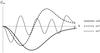 |
Fig. D.2
Illustration of the radial basis elements of the ℓ = 2 Kalnajs basis elements for kKa = 7, defined in Appendix A, which were used in the estimation of the Balescu-Lenard diffusion flux in Sect. 4.2. As the radial index n increases, the basis elements get more and more wound. |
| Open with DEXTER | |
 |
Fig. D.3
Map of |
| Open with DEXTER | |
Appendix E: Sampling of the DF
In order to use the N-body integrator described in Sect. 5, one has to sample the particles according to the DF given by Eq. (49). We introduce the probability distribution function Fsp, normalised to 1 and thanks to which the sampling is performed. This probability DF Fsp is directly proportional to the active distribution function Fstar from Eq. (49), so that we may write ![]() (E.1)where Csp is a normalisation constant which is determined in the upcoming calculations. Because the mapping (E,L) → (Jr,Jφ) from Eq. (12) is not a trivial one, we do not perform the sampling of the stars in the action space (Jr,Jφ), but rather in the (E,L)-space. Moreover, one should pay attention to the fact that the DF Fsp from Eq. (E.1) is a probability distribution function in the (x,v)-space, so that d2xd2vFsp(x,v) is proportional to the number of particles in the infinitesimal volume d2xd2v around the position (x,v). As we want to sample the particles in the (E,L)-space, we introduce the function hsp(E,L) such that dEdLhsp(E,L) is proportional to the number of particles in the volume dEdL around the location (E,L). One can now determine hsp(E,L) as a function of F(E,L). Indeed, we have
(E.1)where Csp is a normalisation constant which is determined in the upcoming calculations. Because the mapping (E,L) → (Jr,Jφ) from Eq. (12) is not a trivial one, we do not perform the sampling of the stars in the action space (Jr,Jφ), but rather in the (E,L)-space. Moreover, one should pay attention to the fact that the DF Fsp from Eq. (E.1) is a probability distribution function in the (x,v)-space, so that d2xd2vFsp(x,v) is proportional to the number of particles in the infinitesimal volume d2xd2v around the position (x,v). As we want to sample the particles in the (E,L)-space, we introduce the function hsp(E,L) such that dEdLhsp(E,L) is proportional to the number of particles in the volume dEdL around the location (E,L). One can now determine hsp(E,L) as a function of F(E,L). Indeed, we have 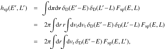 (E.2)using the fact that the tangential velocity satisfies vt = L/r. The last step is then to perform the change of variable vr → E. One has
 ![]() , so that
, so that ![]() . Because the radial velocity can be both positive and negative, Eq. (E.2) takes the form
. Because the radial velocity can be both positive and negative, Eq. (E.2) takes the form 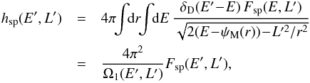 (E.3)where we used the definition (13) of the radial intrinsic frequency Ω1. One can then correctly normalise the probability distribution hsp and determine the value of the constant Csp from Eq. (E.1). One should pay attention to the fact that in addition to the tapering functions Tinner and Touter from Eqs. (48), we also assume that no stars have orbits that extend beyond Rmax. As a consequence, the allowed region in the (E,L)-space has to satisfy two constraints. First of all, the angular momentum Lstar has to satisfy
 ![]() (E.4)Then, for a given value of Lstar, one can show that the energy of the star Estar must satisfy the constraint
(E.4)Then, for a given value of Lstar, one can show that the energy of the star Estar must satisfy the constraint 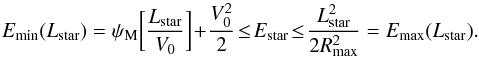 (E.5)These two constraints allow us to completely characterise the (E,L)-space on which the sampling (E,L) has to be performed. One finally has to satisfy the constraint
 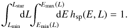 (E.6)Given the parameters presented after Eq. (49), one can numerically determine the value of the constant Csp which reads
![]() (E.7)We may now proceed to the sampling of the coordinates of the particles. Up to the sign of its radial velocity, one star is characterised by the set {Estar,Lstar,Rstar,φstar }. Given that the initial state is axisymmetric, the azimuthal angle of the star can be uniformly sampled between 0 and 2π. The next step is then to successively sample (Lstar,Estar) and finally Rstar, using successive rejection samplings as we now detail.
(E.7)We may now proceed to the sampling of the coordinates of the particles. Up to the sign of its radial velocity, one star is characterised by the set {Estar,Lstar,Rstar,φstar }. Given that the initial state is axisymmetric, the azimuthal angle of the star can be uniformly sampled between 0 and 2π. The next step is then to successively sample (Lstar,Estar) and finally Rstar, using successive rejection samplings as we now detail.
The heart of the rejection sampling is as follows. Let us assume that we want to generate sampling values from a function f(x), from which it is difficult to sample. However, we assume that we have at our disposal another distribution function g(x) from which the sampling is simple, and such that there exists a bound M> 1 satisfying f(x) <Mg(x). The smaller M, the more efficient the sampling. One then has to proceed as follows: sample both a proposal x from g and u uniformly between [ 0;1 ]. One then applies the selection 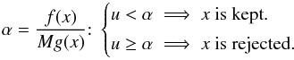 (E.8)In order to have an efficient sampling, one should try to consider a function g close to f.
We may now directly sample (E,L) thanks to this algorithm. The true sampling function is f(E,L) = hsp from Eq. (E.2). The simple sampling function is g(E,L) ∝ 1, defined on the domain characterised by the constraints from Eqs. (E.4) and (E.5). When performing a rejection sampling with such a uniform g(E,L), in order to determine the bound M(E,L), one only has to determine a uniform bound for f(E,L). With the numerical values introduced after Eq. (49), one can check that f(E,L) is such that ![]() (E.9)The final element required to be able to perform the rejection sampling with f(E,L) is to be able to draw uniformly candidate (E,L) in the domains defined by the constraints from Eqs. (E.4) and (E.5), which is equivalent as sampling candidates (E,L) from the uniform probability distribution function g(E,L). To perform this uniform sampling, since the constraints from Eq. (E.5) are expressed for a given value of Lstar, it is more natural to first draw Lstar and then Estar. The probability distribution according to which Lstar has to be drawn is of the form fL(L) ∝ (Emax(L) − Emin(L)). When correctly normalised, it reads
(E.9)The final element required to be able to perform the rejection sampling with f(E,L) is to be able to draw uniformly candidate (E,L) in the domains defined by the constraints from Eqs. (E.4) and (E.5), which is equivalent as sampling candidates (E,L) from the uniform probability distribution function g(E,L). To perform this uniform sampling, since the constraints from Eq. (E.5) are expressed for a given value of Lstar, it is more natural to first draw Lstar and then Estar. The probability distribution according to which Lstar has to be drawn is of the form fL(L) ∝ (Emax(L) − Emin(L)). When correctly normalised, it reads 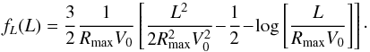 (E.10)To sample L from fL, we use another rejection sampling by introducing the additional simple probability distribution function gL defined as
 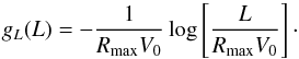 (E.11)It is straightforward to check that fL< (3 / 2) gL, so that we may use the bound ML = 3 / 2 to perform the rejection sampling of Lstar. The final remark is to note that sampling L from gL is simple since its cumulative distribution function
 ![]() can be inverted so as to read
can be inverted so as to read ![]() (E.12)where W-1 is the lower branch of the Lambert function W(x) for x ∈ [ −1 / e ;0 ]. With all these elements, the rejection sampling of Lstar following fL from Eq. (E.10) can be performed.
(E.12)where W-1 is the lower branch of the Lambert function W(x) for x ∈ [ −1 / e ;0 ]. With all these elements, the rejection sampling of Lstar following fL from Eq. (E.10) can be performed.
Once Lstar has been drawn, it only remains to sample uniformly Estar on the interval Estar ∈ [ Emin(Lstar) ;Emax(Lstar) ], as given by Eq. (E.4). Thanks to these uniformly drawn candidates (Estar,Lstar) and the uniform bound from Eq. (E.9), one can perform the rejection sampling from the probability distribution f(E,L).
For Estar and Lstar succesfully sampled, one may then sample the radius Rstar using a similar rejection sampling. The radius has to be sampled according to the probability distribution fR given by 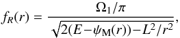 (E.13)so that one has fR ∝ vr. However, one should note that for r → rp/a, one has fR(r) → + ∞, so that the rejection sampling cannot be used without considering a probability DF g which also diverges for r → rp/a. In order to get rid of these divergences, instead of sampling the variable r, we sample the angle u ∈ [ −π/2 ;π/2 ], where we defined the mapping r → u(r) as
 ![]() (E.14)so that one naturally has r(−π/2) = rp and r(π/2) = ra. The probability distribution function from which u has to be sampled is immediately given by
(E.14)so that one naturally has r(−π/2) = rp and r(π/2) = ra. The probability distribution function from which u has to be sampled is immediately given by ![]() (E.15)Using the fact that the maximum of fu is reached for u = π/2, one can then sample u from fu using a rejection sampling with a uniform control probability distribution function gu(u) = 1 /π. Once u is known, it only remains to compute Rstar = r(ustar), so that the sampling of all the required quantities for one star has been performed.
(E.15)Using the fact that the maximum of fu is reached for u = π/2, one can then sample u from fu using a rejection sampling with a uniform control probability distribution function gu(u) = 1 /π. Once u is known, it only remains to compute Rstar = r(ustar), so that the sampling of all the required quantities for one star has been performed.
The final step of the sampling of the particles is to determine the physical coordinates of the particles (x,v) associated with the set {Estar,Lstar,Rstar,φstar }. These physical coordinates are the ones which are given to the N-body integrator. We draw uniformly the sign of the radial velocity εr ∈ {−1,1 }. Because we are considering a disc made only of prograde stars, one immediately obtains that the radial and tangential velocities vr and vt are given by  (E.16)The final step of the transformation to the (x,v)-coordinates is then straightforward, since one naturally has
  (E.17)One should note that the sampling procedure described previously does not correspond to a quiet start procedure (Sellwood 1983), which would lead to a reduction of the initial shot noise within the disc, as briefly discussed in Appendix C, with regard to the validation of the N-body code.
Appendix F: Another test of the scaling with N
One difficulty with the measurement of the scaling with N presented in Sect. 5.2 is that one has to disentangle the contributions from the initial sampling Poisson shot noise present through h0 from Eq. (59) and the effects due to the collisional Balescu-Lenard diffusion scaling through h2 from Eq. (64). Indeed, Poisson shot noise leads to fluctuations of the system DF about its mean value. In order not to be sensitive to such fluctuations, one could only consider fluctuations sufficiently large, i.e. fluctuations caused by an effective secular diffusion rather than caused by inevitable Poisson fluctuations. As a consequence, by restricting ourselves only to large fluctuations, we can get rid of Poisson’s effects. We therefore define the function ![]() as
as 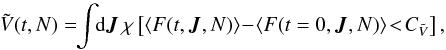 (F.1)where we introduced a threshold
 ![]() . Here χ [·] is a characteristic function equal to 1 if
. Here χ [·] is a characteristic function equal to 1 if ![]() , and 0 otherwise. As a consequence,
, and 0 otherwise. As a consequence, ![]() measures the volume in action space of the regions (depleted from particles, since
measures the volume in action space of the regions (depleted from particles, since ![]() ) for which the mean DF has changed by more than
) for which the mean DF has changed by more than ![]() . For a sufficiently large value of the threshold
. For a sufficiently large value of the threshold ![]() , such a construction allows us not to be polluted by Poisson sampling shot noise. For the initial times, as in Eq. (50), it is straightforward to study the scaling of
, such a construction allows us not to be polluted by Poisson sampling shot noise. For the initial times, as in Eq. (50), it is straightforward to study the scaling of ![]() with t and N.
with t and N.
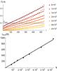 |
Fig. F.1
Top panel: illustration of the behaviour of the function |
| Open with DEXTER | |
Indeed, one can write ![]() (F.2)\newpage
(F.2)\newpage
Introducing ![]() , one can rewrite Eq. (F.2) as
, one can rewrite Eq. (F.2) as ![]() (F.3)Therefore, for a fixed value of N, one expects to observe a linear time dependence of the function
(F.3)Therefore, for a fixed value of N, one expects to observe a linear time dependence of the function ![]() , as illustrated in Fig. F.1. In order to test the scaling of Eq. (F.3) with N, one may proceed as follows. Introducing a threshold value
, as illustrated in Fig. F.1. In order to test the scaling of Eq. (F.3) with N, one may proceed as follows. Introducing a threshold value ![]() , for each value of N, we define the associated threshold time tthold(N) as
, for each value of N, we define the associated threshold time tthold(N) as![]() (F.4)Thanks to the scalings from Eq. (F.3), one immediately obtains that
(F.4)Thanks to the scalings from Eq. (F.3), one immediately obtains that  (F.5)Such a linear scaling of tthold(N) with N is a prediction from the Balescu-Lenard formalism and is nicely recovered in Fig. F.1.
Appendix G: Distributed code description
For the sake of reproducibility, which has been lacking in the context of the linear response of stellar systems, we distribute the linear matrix response code we wrote for this paper both as a Mathematica package6, and a notebook7. The functions therein allow for:
-
The determination as a function of (rp,ra) of the orbits quantites: E, L, Jr, Ω1 and Ω2.
-
The construction of the 2D basis from Kalnajs (1976).
-
The computation of the Fourier transform w.r.t. the angles, i.e. the computation of
 from Eq. (21).
 -
The calculation of the 2D response matrix via Eq. (33).
It has been tested for the isochrone and the Mestel discs. A copy of the code is also available at the CDS.
© ESO, 2015
Current usage metrics show cumulative count of Article Views (full-text article views including HTML views, PDF and ePub downloads, according to the available data) and Abstracts Views on Vision4Press platform.
Data correspond to usage on the plateform after 2015. The current usage metrics is available 48-96 hours after online publication and is updated daily on week days.
Initial download of the metrics may take a while.