| Issue |
A&A
Volume 583, November 2015
|
|
|---|---|---|
| Article Number | A94 | |
| Number of page(s) | 9 | |
| Section | Stellar atmospheres | |
| DOI | https://doi.org/10.1051/0004-6361/201527120 | |
| Published online | 02 November 2015 | |
Online material
Appendix A: Dependence of abundances on the number of lines: the case of Ni
The data used in this work was taken from Adibekyan et al. (2012), which provides chemical abundances for 12 iron-peak and α-capture elements (15 ionized or neutral species).
The lines used are based on the line list of Neves et al. (2009). From the VALD3 online database, 180 lines were carefully selected in the solar spectrum to be: not-blended, have equivalent widths (EW) above 5 mÅ and below 200 mÅ, and be located outside of the wings of very strong lines. Later on, the semi-empirical oscillator strengths for the lines were calculated by calibrating the log gf values to the solar reference of Anders & Grevesse (1989). Moreover, only “stable” lines, which do not show high abundances dispersion (i.e., 1.5 times the rms) from the mean abundance for each element, were selected. In this later test, 451 stars with a wide range of stellar parameters and S/N were used. The selected 180 lines were re-checked in Adibekyan et al. (2012), where several lines were excluded because of the observed abundance trend [X/Fe] with the effective temperature. For more details about the selection of the lines, see Neves et al. (2009) and Adibekyan et al. (2012). Our final line-list consists of 164 lines4.
We stress that the main goal of this work is not to re-check the quality of the lines, nor to provide a range of parameter space (stellar parameters and S/N) where each individual line can be used safely and reliably. Since different authors use different sets of spectral lines and different atomic data for the lines, for us it is more straightforward and scientifically interesting to discuss methods that can, in principle, work effectively for different line lists and be applied to large data sets, as is often the case.
Appendix A.1: Comparing methods
In Adibekyan et al. (2012) the final abundance for each star and element was calculated as the arithmetic mean (AM) of the abundances given by all lines detected in a given star and element after a two-sigma clipping was applied. This is a standard and widely used technique that avoids the errors caused by bad pixels, bad measurements, cosmic rays, and other unknown localized effects. However, this type of outlier removal technique depends on the threshold (2σ in our case) that is applied. There is no clear prescription or theoretical ground for this and the choice ends up being very subjective. The choice of threshold should also depend on the sample size. A simple demonstration of this dependence on sample size is presented by Shiffler (1988), who showed that the possible maximum Z-score (the number of SD a data-point is far from the mean) depends (only) on the sample size and is computed as (n−1)/![]() . From this formula we understand that the maximum deviation that one can obtain in a sample of five points (lines) is 1.79σ, i.e., no outliers can be identified in the data if 2σ-clipping is applied. One can alternatively use median and median absolute deviation (MAD), which is expected to be less sensitive to outliers, or one can apply other outlier removal methods (e.g., Hodge & Austin 2004; Iglewicz & Hoaglin 1993). However, it is very difficult to choose a single method and a criterion that will work efficiently for samples of different sizes. Moreover, when a certain criterion is applied to remove possible outliers, some valid lines from the real distribution may be removed as well. Finally, one should also bear in mind that most of the outlier removal methods are model-dependent, assuming some distributions for the real and outlier data.
. From this formula we understand that the maximum deviation that one can obtain in a sample of five points (lines) is 1.79σ, i.e., no outliers can be identified in the data if 2σ-clipping is applied. One can alternatively use median and median absolute deviation (MAD), which is expected to be less sensitive to outliers, or one can apply other outlier removal methods (e.g., Hodge & Austin 2004; Iglewicz & Hoaglin 1993). However, it is very difficult to choose a single method and a criterion that will work efficiently for samples of different sizes. Moreover, when a certain criterion is applied to remove possible outliers, some valid lines from the real distribution may be removed as well. Finally, one should also bear in mind that most of the outlier removal methods are model-dependent, assuming some distributions for the real and outlier data.
To explore and choose the method that allows a derivation of the most precise final abundances of the elements, we selected Ni for our analysis because it has the largest line list (43 lines). By plotting the individual Ni abundances in the full sample of 1111 stars, we noticed that many of the stars have Ni lines that show deviation from the average value by more than 3σ. To understand if these lines are outliers or just extremes of the distribution (a normal distribution is assumed here) we performed some simple calculations. If one assumes a normal distribution, then a 3σ corresponds to P = 0.003 probability. Since on average we derive Ni abundance from 43 lines, then the probability that we will have at least one “outlier” is of 43 × 0.003 = 0.129. This means that among the 1111 stars, we expect to have about 0.129 × 1111 = 143 stars with one “outlier” line. However, the number of stars that have at least one “outlier” is 626. To estimate the probability of having that many stars with at least one “outlier” we used binomial probability distribution. The probability that more than 200 stars (any number above 200) can have an “outlier” is already 8×10⁻⁷. This means that, under our assumption of Gaussian distribution of the abundances derived from different lines, some of the lines which show large dispersion (>3σ) can be real outliers of different origin and are not just coming from the wings of the Gaussian distribution. We note, that the results of this test do not depend on the applied threshold (3σ in this case).
Fortunately, if the line list is large, the possible outliers do not greatly affect the final (mean) abundance. We first tested three different outlier removal methods, namely σ-clipping (e.g., Shiffler 1988), modified Z-score (Iglewicz & Hoaglin 1993), and median-rule (Carling 1998) on our data. The modified Z-score method is similar to n × σ-clipping, but instead of mean and SD, the median and MADe5 are used. Median-rule is a modification of Tukey’s (boxplot) method (Tukey 1977), and defines outliers as points that lie further than median ± k × IQR, where IQR is the interquartile range. We varied the k to { 2,2.5,3 } for the σ-clipping and median-rule, and k = { 2.5,3,3.5 } for the modified Z-score. The selected values of k are within the intervals suggested in the above-cited references.
A potential difficulty that one faces when trying to remove outliers is the so-called masking and swamping effects. Removal of one outlier changes the “status” of the other data points (Acuna & Rodriguez 2004). This means that it is advisable to remove one outlier at a time and apply the criteria recursively. However, it is not obvious when the outlier removal criteria should be stopped (the problem also exists when all the outliers are removed at once). Two approaches were considered in our tests when modified Z-score method was used: i) remove all the outliers at once (referred to as MADe technique in the remainder of the paper) and ii) remove one outlier at a time and then apply the criterion again iteratively (hereafter referred to as MAD![]() technique). For the second approach we allowed a maximum number of ten iterations, although in most cases, a lower number of iterations were needed (depending, of course, on the threshold accepted).
technique). For the second approach we allowed a maximum number of ten iterations, although in most cases, a lower number of iterations were needed (depending, of course, on the threshold accepted).
|
Fig. A.1
Difference in [Ni/H] and σ[Ni/H] when WM and AM without outlier removal methods are applied (left). The same as in the left panel, but the parameters are derived using WM and MAD |
|
| Open with DEXTER | |
Outlier removal is not the only method used to characterize an underlying distribution in a data set. An example is the weighted least-squares regression to minimize the effects of outlier data (Rousseeuw & Leroy 1987). The last method that we use to calculate the final abundance and its line-to-line scatter is the WM and weighted SD. As a weight we used the (inverse) distance from the median value in terms of SD and then binned it. Using MAD and SD in the calculations of the weight on the average give very similar results, but if the values of more than the half of the points (lines) are the same (which can happen when the number of lines is small) then MAD is by definition zero and cannot be used to calculate the weight. Since the distance of the median point from the median is zero, the weight of that line would be infinite. To avoid giving a very high weight to the points that are initially close to the median (the final value would, by construction, be very close to the median), we decided to bin the distances with an interval of 0.5SD. For example, a 0.5 × SD weight was given to the lines that are 0 to 0.5 SD away from the median. Similarly, a 1 × SD weight was given to the lines lying at distances of 0.5 to 1 × SD, and so on.
Difference in Ni abundances when WM method and other methods are applied for the derivation of Ni.
The results of our tests are summarized in Table A.1. The test showed that all the outlier removal methods give a mean, final abundance similar to that of the WM. Since the number of lines is relatively large, the impact of possible outliers is small, and all the values were also similar to the abundance calculated by the AM of all the points. However, we note that, when the lowest thresholds were set to remove outliers, some stars showed deviations in the final abundance from the mean abundance derived from different methods. This was because of the large number of removed “outliers”. Another important point to stress is that, when outlier removal methods were applied with low thresholds, the line-to-line scatter (which is usually used as an error estimate of the final abundance) was usually small, which was expected.
|
Fig. A.2
Difference between original Ni abundance and Ni abundances derived with only 2, 10, and 30 Ni lines. |
|
| Open with DEXTER | |
|
Fig. A.3
Average deviation from the original Ni abundance for 1111 stars versus number of lines that were used for the abundance derivations. The right panel is the zoom of the left plot, limited to only six lines. Different techniques that were used in the calculations are mentioned in the plots. |
|
| Open with DEXTER | |
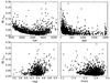 |
Fig. A.4
Dependence of the average deviation from the original Ni abundance for 1111 stars versus stellar parameters and S/N. The abundance deviation represents the difference between original Ni abundance and Ni abundance derived with only 2 lines. |
| Open with DEXTER | |
From these tests (and further tests presented next in this work), we conclude that the best way to calculate the final abundance and its error is to use the WM. In this case, the weight of real outliers (extremes) is low, and the final abundance is not affected. With this approach, we also do not reduce the scatter by artificially removing points from the distribution. In Fig. A.1, we plot the distribution of the Ni abundance and its error (line-to-line dispersion) differences when WM and AM method is applied (left plot), and when WM and MAD![]() (median ± 3MAD) criteria are applied (right plot). From the plot and table, it is very clear that, when the number of lines is large, different methods for outlier removal (or not) provide very similar results for Ni abundances, however the error associated with these values depends on the method. In particular, Fig. A.1 (left plot) shows that line-to-line scatter of [Ni/H] is always larger when the Ni abundance is calculated by the AM than when the WM method is used (the difference in σ[Ni/H] is always positive). The righthand panel of the same figure shows that the difference in σ[Ni/H] is usually small and can be both positive and negative when Ni abundance is calculated by WM and MAD
(median ± 3MAD) criteria are applied (right plot). From the plot and table, it is very clear that, when the number of lines is large, different methods for outlier removal (or not) provide very similar results for Ni abundances, however the error associated with these values depends on the method. In particular, Fig. A.1 (left plot) shows that line-to-line scatter of [Ni/H] is always larger when the Ni abundance is calculated by the AM than when the WM method is used (the difference in σ[Ni/H] is always positive). The righthand panel of the same figure shows that the difference in σ[Ni/H] is usually small and can be both positive and negative when Ni abundance is calculated by WM and MAD![]() .
.
A word of caution should be added at this point. In the methods that we tested to remove “outliers”, as well as in the WM technique we assume that the distribution of the abundances (or the distribution of the errors on abundances) is symmetric6. However, as was shown in Bertran de Lis et al. (2015), for very weak lines with an assumption of local thermodynamic equilibrium (LTE), the distribution of uncertainties of abundances is asymmetric. The authors also showed that this effect depends on the S/N and is negligible for lines with EW greater than 8 mÅ, regardless of S/N. However, since in all the methods are based on the same hypothesis, the WM technique remains favorable for us.
Appendix A.2: Abundance precision dependence on the number of lines
To evaluate the impact of the number of lines (used for abundance derivations) on the abundances, we did the following simple tests. For each star in the sample, we randomly drew N Ni lines (N = 2, 3, ..., 42) and calculated the Ni abundance. We used the above-mentioned WM technique for the calculation of the abundances. Then we compared the resulting abundances with the supposed Ni abundance value (derived by using all 43 available lines and the WM technique). If the number of possible combinations is less than 1000, we considered all the possible combinations of lines, otherwise we drew N = 1000 random, but different, combinations of lines7.
In Fig. A.2, we plot an example (for two stars) of the distribution of the differences in Ni abundances (Δ[Ni/H]) when three different number of Ni lines (2, 10, and 30 lines) and all the available lines are used. The stars have different stellar parameters and different S/N in the spectra. The plot shows that, when the number of lines is increased, the abundance difference decreases. It also shows that, while the Δ[Ni/H] is close to zero in most of cases/trials, it is possible to obtain very large differences when only two lines are used (even for very high S/N data).
We did the aforementioned computations for all the 1111 stars and for each number of lines we calculated the standard deviation of Δ[Ni/H] distribution – σdev. In Fig. A.3, we plot the dependence of the average of the σdev for all 1111 stars as a function of the number of lines. In the plot, we limited ourselves only to examples of four techniques with different thresholds so as not to overload the figure, while applying all the techniques and thresholds presented in Table A.1. Moreover, since the size of the sample (lines) varies in these tests, we also decided to test lower outlier removal thresholds: k = 1.5 for σ-clipping and median-rule methods, and k = 2 for modified Z-score methods.
Figure A.3 shows the range of possible deviations (1σ deviation if the distribution was a Gaussian) from the original value for a given random star, when randomly draw N lines are used. It clearly shows that the deviation decreases very steeply with the number of lines and becomes less than 0.01 dex when more than 15 lines are used.
In the righthand panel of Fig. A.3, we show that there is a subtle difference between different outlier removal techniques for a number of lines less than or equal to six. It clearly shows that the smallest average deviation is obtained when the WM is used. We note that other tests show similar results with different thresholds. The low thresholds for outlier removal techniques give results closer to those obtained by using WM for a small number of lines. However, when low thresholds are considered for a large number of lines, the final results deviate from the abundances obtained by using the WM method. This is because of the high number of excluded lines. For the remainder of the paper we use abundances calculated by the WM method if another method is not specified. Here we should stress again that we plot the possible deviations of Ni abundances that were averaged for 1111 stars. While these average values are low, the deviations for individual stars can be very significant (as demonstrated in Fig. A.2).
It is natural to expect that the observed deviations should depend chiefly on the quality of the data (e.g., S/N) and also on the atmospheric parameters of the stars. This is because, for example, spectral lines in cooler stars’ spectra are usually more blended, and also because, for example, different lines form at different layers of the atmospheres and have different sensitivities to the non-LTE effects. In Fig. A.4, we plot the dependence of the average σdev on the stellar atmospheric parameters and on the S/N, when only two lines were used to derive the abundances. The plot shows that there is only a strong and clear dependence on Teff. This result is to be expected since, at low temperatures, the spectra of cool stars are crowded and line-blending plays a stronger role. Lowest metallicity stars and stars with the lowest S/N also show somewhat larger deviations. It is interesting to note that, even if the S/N is very high, it is possible to obtain a Ni abundance of up to 0.1 dex different from the original abundance, depending on stellar parameters, when only two Ni lines are used.
Appendix B: [X/Fe] star-to-star scatter: dependence on the number of lines
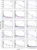 |
Fig. B.1
Dependence of [X/Fe] star-to-star scatter for solar analogs with [Fe/H] = 0.0 ± 0.10 dex on the number of lines. Red triangles show the scatter when the individual abundances are calculated as an AM and the blue squares indicate the scatter in [X/Fe] when the WM method was used for the abundance derivation. The black dots show the [X/Fe] scatter for each individual line that was used to derive [X/H]. The error bars indicate the dispersion of possible combinations of the lines. |
| Open with DEXTER | |
© ESO, 2015
Current usage metrics show cumulative count of Article Views (full-text article views including HTML views, PDF and ePub downloads, according to the available data) and Abstracts Views on Vision4Press platform.
Data correspond to usage on the plateform after 2015. The current usage metrics is available 48-96 hours after online publication and is updated daily on week days.
Initial download of the metrics may take a while.