| Issue |
A&A
Volume 583, November 2015
|
|
|---|---|---|
| Article Number | A61 | |
| Number of page(s) | 16 | |
| Section | Cosmology (including clusters of galaxies) | |
| DOI | https://doi.org/10.1051/0004-6361/201526330 | |
| Published online | 28 October 2015 | |
Online material
Appendix A: Anti-aliasing filter
Binning the continuous galaxy density field onto a grid may be characterised as a smoothing operation followed by discrete sampling (Hockney & Eastwood 1988). In the simplest approach, if particles are assigned to the nearest grid point (NGP) the smoothing kernel W(x) has a top-hat shape with the dimension of the grid cell. More extended kernels can be chosen that distribute the weight of the particle over multiple cells. Common assignment schemes include cloud-in-cell (CIC) and triangle-shaped-cell (TSC) which correspond to iterative smoothing operations with the same top-hat filter. Smoothing the field damps small scale power, but better localises the signal in k-space which is beneficial in Fourier analyses.
A consequence of using the fast Fourier transform (FFT) algorithm is that the signal must be discretised onto a finite number of wave modes or equivalently that periodic boundary conditions are imposed. The observed power is thus a sum of all harmonics of the fundamental wavelength which are known as aliases (Jing 2005; Hockney & Eastwood 1988): 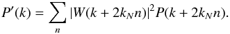 (A.1)As long as the signal is sufficiently well sampled and band-limited, meaning that there is no power above the Nyquist frequency, the signal may be recovered without error. However, most signals of interest are not band limited, and so after sampling onto the grid, the harmonics overlap and the signal cannot be exactly recovered.
The ideal anti-aliasing filter in k-space is the top-hat that cuts all power above the Nyquist frequency. However, the signal cannot be localised both in k-space and in position-space and a sharp cut in k-space will distribute the mass of a particle over the entire grid.
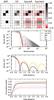 |
Fig. A.1
Top panel: an illustration of the mass-assignment kernels in two-dimensions: a hard k-space cut (Sup hard), a soft k-space cut (Sup soft), nearest-grid-point (NGP) and cloud-in-cell (CIC). The lower three panels give a comparison of the kernel functions (in one dimension) for various mass assignment schemes. Top: the kernels in Fourier space. The Nyquist frequency is 1 pixel-1 on the scale. Middle: the kernels in position space. Bottom: the cumulative power of each kernel in position space. |
| Open with DEXTER | |
A practical implementation of the ideal filter was developed by Jasche et al. (2009). The method involves first super-sampling the field by assigning particles to a grid with resolution higher than the target grid. Transforming to Fourier space via FFT, the high resolution grid is filtered setting to 0 all modes above the target Nyquist frequency. Finally the grid is transformed back to position-space and down sampled to the target grid. The technique is very efficient with the additional trick that the down-sampling step can be carried out by the inverse FFT by cutting and reshaping the Fourier grid.
The algorithm of Jasche et al. (2009) is limited only by the memory needed to apply the FFT on the high resolution grid, so it is competitive with common position-space cell assignment schemes. However, the sharp cut in k-space leads to an extended, oscillatory distribution in position-space. Such a decentralised and unphysical cell assignment is undesirable for estimation of the density field.
An alternative approach was taken by Cui et al. (2008) who introduce the use of Daubechies wavelets to approximate the ideal filter while keeping compactness in position-space. We do not consider this technique here because the centre of mass of the wavelets adopted is offset from the particle position and so they are not well suited for estimation of the density field.
As a compromise, we test a smooth cutoff with a k-space filter with the form:  (A.2)The parameter α adjusts the sharpness of the cut: we test α = 100 (Sup hard) and α = 8 (Sup soft).
Figure A.1 shows the comparison of the mass assignment schemes including the super-sampling technique. We see that the hard cut (Sup hard) leads to ringing in position-space (the transform is the sinc function). The amplitude is significantly reduced when the parameter α = 8 (Sup soft) and the first peak is more compact than CIC. In k-space, the filter remains nearly 1 to ~0.7kN while NGP, CIC and TSC functions are dropping. Beyond the Nyquist frequency, the soft cut-off kernel drops faster than TSC without oscillatory behaviour. The bottom panel of A.1 shows the cumulative power ![]() . We see that soft-cut off scheme has compactness similar to CIC and NGP, while the latter schemes severely damp the total power.
. We see that soft-cut off scheme has compactness similar to CIC and NGP, while the latter schemes severely damp the total power.
Figure A.2 compares the aliased power in the power spectrum measurement. The top four panels show the shot noise power multiplied by the kernels. The principal contribution (n = 0) and the first harmonic (n = −1) are plotted along with the full sum of all harmonics. We see for instance, that the power measured with the NGP scheme mixes power from all harmonics. The hard cut-off filter performs nearly ideally with no aliasing effect. The soft cut-off also performs well matching the aliasing characteristics of the TSC scheme.
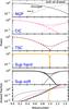 |
Fig. A.2
A comparison of the shot noise power as a function of wavenumber under various mass assignment schemes. The Nyquist frequency is 1 pixel-1 on the scale. The top four plots show the principal component (thick line), the n = −1 harmonic and the sum of all harmonics (thin line). The bottom frame shows the fraction of aliased power for each assignment scheme. |
| Open with DEXTER | |
To implement the soft cut-off filter we use the following practical super-sampling recipe:
-
1.
Assign particles to a grid with resolution increased by a factorf. The assignment is done with the CIC scheme. We set f = 8.
-
2.
Transform the field to Fourier space with the FFT.
-
3.
Multiply Fourier modes by the k-space filter.
-
4.
Transform back to position space with the inverse-FFT.
-
5.
Take a sample of the grid every f cells to down-sample to the target resolution.
Appendix B: Gibbs sampler
Here we give the algorithms used to sample from the conditional probability functions.
Appendix B.1: Sampling the density field
Using a galaxy survey we count galaxies in a given sample l and construct the spatial field Nl which is a vector of length ncells. We will write the set of m galaxy samples (e.g. different luminosity and redshift bins) as { Nl } ≡ { Nl1,Nl2,...,Nlm }. Each sample l has a corresponding mean density ![]() and bias bl.
and bias bl.
We write the conditional probability for the underlying density field δ as 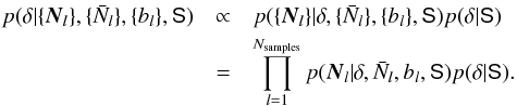 (B.1)To write the last line we use the property that the number counts of different samples l are conditionally independent but depend on the common underlying density field.
For clarity we now explicitly index the cells with subscript i. We adopt a Gaussian model for the number counts and write the log of the likelihood log p ∝ χ2 as 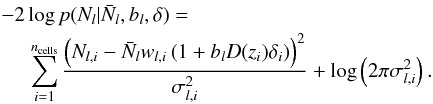 (B.2)The variance of counts is generalised as
 ![]() and may be different from the Poisson expectation
and may be different from the Poisson expectation ![]() due to the mask and anti-aliasing filter. However, we neglect noise correlations between cells which would introduce off-diagonal terms. The sums are carried out over cells with variance
due to the mask and anti-aliasing filter. However, we neglect noise correlations between cells which would introduce off-diagonal terms. The sums are carried out over cells with variance ![]() .
.
Next we consider the density field prior. We set a Gaussian model giving 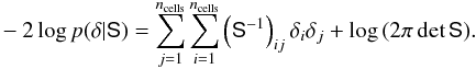 (B.3)The correlation function of δ is given by the anisotropic covariance matrix S. In Fourier space the matrix is diagonal and given by Eq. (10). When writing the posterior we now drop the terms that do not depend on δ giving
 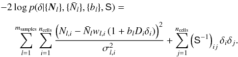 (B.4)Differentiating the log posterior with respect to δ we find the equation for the maximum a posteriori estimator which is also called the Wiener filter. The estimate
 ![]() is given by
is given by 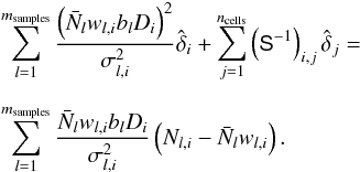 (B.5)It is informative to point out how the Wiener filter operation combines the galaxy subsamples. The right hand side of Eq. (B.5) shows the weighted combination, given by
 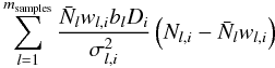 (B.6)where we consider cell i and the sum is over galaxy samples indexed by l. The subsamples are being weighted by their relative biases bl. This form of weighting for the density field was derived by Cai et al. (2011) and is optimal in the case of Poisson sampling but also matches the weights for the power spectrum (Percival et al. 2004).
To generate a residual field δr with the correct covariance we follow the method of Jewell et al. (2004). We draw two sets of Gaussian distributed random variables with zero mean and unit variance: w1,i and w2,i. The residual field is then found by solving the following linear equations. 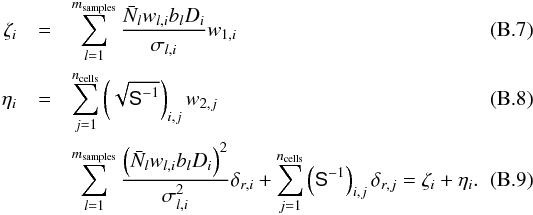 The final constrained realisation is given by the sum
 ![]() .
.
The terms including the signal covariance matrix are computed in Fourier space where the matrix is diagonal. The transformation is done using the Fast fourier transform algorithm. We solve Eqs. (B.5) and (B.9) using the linear conjugate gradient solver bicgstab provided in the SciPy python library1.
Appendix B.2: Sampling the signal
The posterior distribution for the signal is ![]() (B.10)We take a flat prior leaving p(S | δ) ∝ p(δ | S) which is given by Eq. (B.3). This is recognised as an inverse-Gamma distribution for S which can be sampled directly (Kitaura & Enßlin 2008; Jasche et al. 2010b).
(B.10)We take a flat prior leaving p(S | δ) ∝ p(δ | S) which is given by Eq. (B.3). This is recognised as an inverse-Gamma distribution for S which can be sampled directly (Kitaura & Enßlin 2008; Jasche et al. 2010b).
We parametrise the signal in Fourier space as the product of the real-space power spectrum and redshift-space distortion model (Eq. (10)). We sample the parameters in two steps. First we fix β and σv and draw a real-space power spectrum from the inverse-gamma distribution.
The normalisation of the power spectrum is fixed by 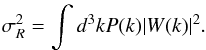 (B.11)In the regime where shot noise is more important than cosmic variance, this method of sampling is inefficient. An alternative sampling scheme was proposed to improve the convergence (Jewell et al. 2009; Jasche et al. 2010b). The new power spectrum is drawn making a step in both P and δ such that
 ![]() . The consequence is that the conditional posterior p(P | δ) is unchanged but the data likelihood is modified through δ. We perform a sequence of Metropolis-Hastings steps to jointly draw P and δ. We alternate between the two modes for sampling P on each step of the Gibbs sampler.
. The consequence is that the conditional posterior p(P | δ) is unchanged but the data likelihood is modified through δ. We perform a sequence of Metropolis-Hastings steps to jointly draw P and δ. We alternate between the two modes for sampling P on each step of the Gibbs sampler.
The redshift-space distortion parameters β and σv are next sampled jointly. These parameters are strongly degenerate on the scales we consider. To efficiently sample these we compute the eigen decomposition of the Hessian matrix to rotate into a coordinate system with two orthogonal parameters. We evaluate the joint probability over a two-dimensional grid in the orthogonal space. Finally we use a rejection sampling algorithm to jointly draw values of β and σv.
Appendix B.3: Sampling galaxy bias
The bias is sampled in the manner described by Jasche & Wandelt (2013b). The conditional probability distribution for the bias of a given galaxy sample is a Gaussian with mean given by: 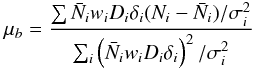 (B.12)and variance
 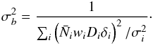 (B.13)After drawing a value from a Gaussian distribution with the given mean and variance, it is limited to the range 0.5 <b< 4.0.
Appendix B.4: Sampling mean density
We take a Poisson model for the mean density. Taking a uniform prior we have  Keeping only terms that depend on
 ![]() we have
we have 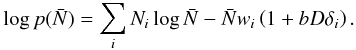 (B.16)We draw a sample from this distribution by computing the likelihood over a grid of values and using a rejection sampling algorithm.
Appendix C: Convergence analysis
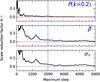 |
Fig. C.1
Gelman-Rubin convergence diagnostic R computed from a single mock catalogue with 10 chains. |
| Open with DEXTER | |
The Gelman-Rubin convergence diagnostic (Gelman & Rubin 1992; Brooks & Gelman 1998) involves running multiple independent Markov chains and comparing the single-chain variance to the between-chain variance. The scale reduction factor R is the ratio of the two variance estimates. In Fig. C.1 we show this convergence diagnostic for three parameters: the power spectrum at k = 0.2h Mpc-1, the distortion parameter β and the velocity dispersion σv. These parameters are the slowest to converge. The R factor is computed up to a given maximum step i in the chain after discarding the first i/ 2 steps. We consider the chain to be properly “burned-in” when R< 1.2. Based on this diagnostic we set the maximum step in our analysis to be 2000 and discard the first 1000 steps.
© ESO, 2015
Current usage metrics show cumulative count of Article Views (full-text article views including HTML views, PDF and ePub downloads, according to the available data) and Abstracts Views on Vision4Press platform.
Data correspond to usage on the plateform after 2015. The current usage metrics is available 48-96 hours after online publication and is updated daily on week days.
Initial download of the metrics may take a while.