| Issue |
A&A
Volume 582, October 2015
|
|
|---|---|---|
| Article Number | A31 | |
| Number of page(s) | 32 | |
| Section | Interstellar and circumstellar matter | |
| DOI | https://doi.org/10.1051/0004-6361/201424955 | |
| Published online | 30 September 2015 | |
Online material
Appendix A: H i component separation
We have developed a careful kinematical separation of the four H i structures present within the analysis region, namely:
-
the H i gas associated with thestar-forming CO clouds of the Chamaeleon complex at velocitiesbetween about −4 and + 15 km s-1;
-
the gas in an intermediate velocity arc (IVA), crossing the whole region around −25° in latitude, at negative velocities down to −40 km s-1;
-
the background H i lying at high altitude above the Galactic disc, at velocities below about + 170 km s-1;
-
gas in the LMC and its tidal tails at the highest velocities.
These components are visible in Fig. A.1.
Because of the broad widths of H i lines, the procedure aims to correct the velocity spillover from one component to the next in the column-density derivation. To do so for each direction in the sky, we have: detected all significant lines in the measured H i spectrum; fitted them with pseudo-Voigt profiles; used the line centroids in velocity to distribute the lines between the components; and integrated each line profile to add its contribution to the column-density map of the relevant component.
The core of the method is based on fitting every spectrum in brightness temperature, TB(v), with a sum of lines across the whole −164.1 ≤ v ≤ 409 km s-1 velocity interval exhibiting significant line emission. The first step is to find the number and approximate velocity of the lines to be fitted. For each (l,b) pixel direction, we have smoothed the spectrum in velocity with a Gaussian kernel of 1.48 km s-1. We have measured the rms dispersion in temperature, Trms, outside the bands with significant emission. We have clipped the data to zero outside regions with T(v) >Trms in 3 adjacent channels. The clipping limits the number of fake line detections triggered by strong noise fluctuations in bands devoid of emission. We have then computed the curvature d2TB/ dv2 in each channel by using the 5-point-Lagrangian differentiation twice. We have detected the line peaks and shoulders by finding the negative minima in d2TB/ dv2. We have eliminated peak detections caused by the edges of the clipped bands. An average line FWHM of 8.2 km s-1 was found in the line fits. We have merged potential lines when separated by less than one half width at half maximum (HWHM) in velocity. Weak lines (Tpeak< 3 K) were also merged when closer than one FWHM in order to limit the number of fake detections on noise fluctuations in faint line wings. When merging lines, the new velocity centroid was set to the average between the parent velocities. The final number of detected peaks and shoulders and their velocities have been used as input parameters for fitting multiple lines across the spectrum.
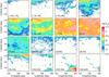 |
Fig. A.1
Maps of the NH i column densities (in cm-2) obtained at 14.́5, resolution from the GASS survey for optically thin emission and integrated over contiguous velocity intervals between the values given in km s-1 on the lower left corner of each map. |
| Open with DEXTER | |
We have fitted each spectrum with a sum of pseudo-Voigt line profiles, one for each detected peak or shoulder. Such a profile combines a Gaussian and a Lorentzian with the same velocity centroid, width, and height, and a relative weight that spans the interval from 0 (pure Gaussian) to 1 (pure Lorentzian). The velocity centroid was allowed to move within ± 3.3 km s-1 (± 4 channels) around the original peak velocity. We have manually checked the precision of many fits across the region. All fits were checked to yield a total line intensity to better than 80−90% of the data integral over the whole spectrum.
In order to preserve the total H i intensity observed in each direction, the small residuals (positive and negative) between the observed and modelled spectra have been distributed between the lines in proportion to the height of each line at each velocity. The line profiles have been corrected accordingly and integrated for a given choice of spin temperature to correct the resulting column-density for the H i optical depth.
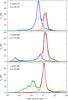 |
Fig. A.2
H i GASS spectra, in brightness temperature, measured toward the three directions indicated on the plots. The best line fits attributed to the local (red), IVA (blue), and Galactic (green) components sum up as the black curve, which closely follows the original data. The grey lines indicate the central velocity and temperature of the individual lines that contribute to a component. |
| Open with DEXTER | |
Each line was attributed to one of the four components according to its velocity centroid in the (l,b) direction. The spatial separation between the IVA and Galactic disc components runs along a broken line of minimum intensity starting at b = −12° at low longitude, reaching ![]() at l = 300°, and moving up to b ≃ −16° at the highest longitude; the frontier can be seen in Fig. 2. Lines pertaining to the local Chamaeleon clouds were selected at −4 km s-1≤ v< 14.8 km s-1 for latitudes below this curve, and at −7.4 km s-1≤ v< 14.8 km s-1 above the border. The lines of the IVA cloud were selected in the −40 km s-1≤ v< −4 km s-1 interval at latitudes below the curve. The latitude cut between the Galactic disc and LMC components runs linearly from
at l = 300°, and moving up to b ≃ −16° at the highest longitude; the frontier can be seen in Fig. 2. Lines pertaining to the local Chamaeleon clouds were selected at −4 km s-1≤ v< 14.8 km s-1 for latitudes below this curve, and at −7.4 km s-1≤ v< 14.8 km s-1 above the border. The lines of the IVA cloud were selected in the −40 km s-1≤ v< −4 km s-1 interval at latitudes below the curve. The latitude cut between the Galactic disc and LMC components runs linearly from ![]() to
to ![]() . The LMC lines were selected at v ≥ 131.9 km s-1 below the latitude cut and at v ≥ 174 km s-1 for all latitudes. The rest of the data was attributed to the Galactic disc component. A selection of spectra is given in Fig. A.2 to illustrate the separation of the local, IVA, and Galactic components.
. The LMC lines were selected at v ≥ 131.9 km s-1 below the latitude cut and at v ≥ 174 km s-1 for all latitudes. The rest of the data was attributed to the Galactic disc component. A selection of spectra is given in Fig. A.2 to illustrate the separation of the local, IVA, and Galactic components.
We have summed the column densities derived for each line associated with a component to produce the maps of Fig. 2. We have tested different velocity cuts around −4 km s-1 between the local and IVA clouds. A change of 1 or 2 km s-1 changes the related maps by 3 to 6% in total mass, mostly in the overlap region near l = 283° and b = −25°. The overall structure and contrast in each map, which drive the correlation studies, remain largely unchanged.
Appendix B: H i spin temperature
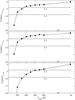 |
Fig. B.1
Evolution of the log-likelihood ratios of the γ-ray fits with the H i spin temperature, using the four independent energy bands in the γ + AVQ (top), γ + τ353 (middle), and γ + R (bottom) analyses. |
| Open with DEXTER | |
For all analyses and for each energy band, we have found that the maximum likelihood value of the γ-ray fit increases with decreasing H i opacity, thus with increasing spin temperature. The data in each band being independent, one can sum the log-likelihoods of each fit to constrain the spin temperature. Figure B.1 indicates that uniform temperatures of TS> 340 K, >300 K, and >640 K are preferred at the 2σ confidence levels for the γ + AVQ, γ + τ353, and γ + R analyses, respectively. The maximum in brightness temperature in the whole data cube is 152 K. This indicates that optically thin conditions largely prevail across the whole velocity range.
In view of these results and with the added arguments that the CR spectrum inside the three H i structures is close to the local one and that the γ-ray intensities have been shown to scale linearly with NH i to higher, less transparent, column densities in more massive clouds (Ackermann et al. 2012b), so that γ rays apparently trace all the H i gas, we follow the γ-ray results and consider the optically thin H i case as that which best represents the data.
Appendix C: CO calibration checks
Checks on the NANTEN data cube have revealed several artefacts that we have corrected before integrating the spectra to obtain the WCO intensities given in Fig. 2. We have removed significant negative lines, probably caused by the presence of a line in the off band in frequency-switching. High-order polynomial residuals were also present in the baseline profiles outside the main CO lines. They did not average out to zero in the WCO map, so we have filtered them from the regions void of significant CO intensity. Moment-masking is commonly used to clean H i and WCO maps (Dame 2011). It was not applicable here because the residuals, unlike noise, extended over several contiguous channels. We have filtered the original WCO map using the multiresolution support method implemented in the MR filter software (Starck & Pierre 1998), with seven scales in the bspline-wavelet transform (à trous algorithm). For the Gaussian noise of WCO, denoising with a hard 4σ threshold led to robust results. The final map shown in Fig. 2 is composed of the original, unfiltered, WCO intensity where the filtered one exceeded 1 K km s-1, and of the filtered intensity outside these faint edges. Particular attention was paid to preserve the faint cloud edges which hold a fair fraction of the cloud mass because of their large volume.
Figure C.1 illustrates the correlations found between the WCO intensities measured over the region with NANTEN (after the corrections described above), with CfA from the moment-masked, fully sampled observations of the Chamaeleon complex (Boulanger et al. 1998), and with Planck (Planck Collaboration XIII 2014). It shows that the data from the PlanckTYPE 1 map is too noisy for our purpose. The other data sets show tight correlations. The correlation coefficients and the slope and intercept of the regression lines are given in Table C.1. They indicate that the PlanckTYPE 3 method systematically overpredicts the intensities in this region compared to the consistent yield of both radio telescopes. An earlier comparison of the NANTEN and CfA surveys across the sky had found 24% larger intensities on average in the NANTEN maps (Planck Collaboration XIX 2011). Figure C.1 shows that the NANTEN and CfA photometries fully agree in the Chamaeleon region. The data are consistent with a unit slope over the whole intensity range. The intercept is compatible with the sensitivity of the NANTEN observations, which varies between 1.5 and 2 K km s-1 across the region.
Linear regression parameters and correlation coefficients between the WCO intensities measured with NANTEN, CfA, and Planck.
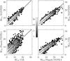 |
Fig. C.1
Correlations and linear regressions between the NANTEN, CfA, and PlanckTYPE 3 and TYPE 1 WCO intensities in the analysis region. The data are sampled at 0.̊125 and the intensities are given in K km s-1. The best-fit slopes are given in Table C.1 |
| Open with DEXTER | |
Appendix D: independent γ-ray and dust fits without DNM templates
In order to check for the presence of substantial amounts of gas not traced by the H i and CO line intensities in the independent γ-ray and dust data sets, we have fitted the γ-ray and dust data with models that do not include a DNM template. All the other components described in Sects. 3.2 and 3.3 have been kept free. The resulting best fits are of significantly lower quality than those obtained with models including the DNM (see Sect. 4). The residual maps, however, are interesting in that they exhibit comparable regions of positive residuals in the independent dust and γ-ray data, as shown in Fig. D.1.
We also note that, in the absence of a DNM template, the best fits yield systematically larger contributions from the H i and CO components than in models that include the DNM. These components, in particular the CO one, are amplified to partially compensate for the missing gas structure. We find 4−13% larger γ-ray emissivities for the local H i and IVA components, and 22% to 57% larger CO γ-ray emissivities. The dust fits respond the same way, with 7−12% larger AVQ/NH, 9−15% larger opacities and 4−7% larger specific powers for the local H i and IVA components, and 25% to 40% larger CO contributions. As a consequence, the best-fit models often over-predict the data toward the CO clouds (see the negative residuals toward Cha II+III and Cha East I and II in Fig. D.1). These results prompted us to iterate the construction of DNM templates between the γ-ray and dust analyses in order to reduce the DNM bias on the determination of the H i and CO parameters.
 |
Fig. D.1
Maps of residuals (data minus best-fit model, in sigma units) obtained when fitting the γ-ray, AVQ, R, or τ353 data (clockwise) with optically thin H i and WCO, but no DNM. In all plots, the grey contours outline the shape of the CO clouds at the 2.3 K km s-1 level. |
| Open with DEXTER | |
Appendix E: Best-fit interstellar coefficients
See Table E.1.
Best-fit coefficients of the γ-ray models (q for each energy band) and of the dust models (y) for the γ + AVQ (top), γ + τ353 (middle), and γ + R (bottom) analyses.
© ESO, 2015
Current usage metrics show cumulative count of Article Views (full-text article views including HTML views, PDF and ePub downloads, according to the available data) and Abstracts Views on Vision4Press platform.
Data correspond to usage on the plateform after 2015. The current usage metrics is available 48-96 hours after online publication and is updated daily on week days.
Initial download of the metrics may take a while.