| Issue |
A&A
Volume 582, October 2015
|
|
|---|---|---|
| Article Number | A30 | |
| Number of page(s) | 29 | |
| Section | Cosmology (including clusters of galaxies) | |
| DOI | https://doi.org/10.1051/0004-6361/201424790 | |
| Published online | 30 September 2015 | |
Online material
Appendix A: SPIRE band-merging procedure
Percentages of SPIRE sources matched at 250 and 500μm from the 350μm input SPIRE catalogue, and the frequency of matches (i.e., number of sources found per 350μm source).
We describe here the details of the band-merging procedure, highlighted in Sect. 3.3.
First step: positional optimization of blind catalogues using shorter wavelength data.
-
Apply a 4σ cut to the 350μm blind catalogue obtained with StarFinder (Sect. 3.2). This cut is imposed to obtain a high purity of detections.
-
Match by position the 350μm sources to the 250μm catalogue, within a radius of one 250μm FWHM.
The following depends on whether there are 0, 1, 2, or more matches:
-
if zero sources are found at 250μm, this is a non-detection at 250μm;
-
if one source is found, we take this source to be the 250μm counterpart;
-
if two sources are found, we replace the position of the 350μm unique source by the two positions of the 250μm sources (the 350μm flux density will be measured later) and take the two 250μm flux densities;
-
we apply the same procedure for triply or more matched sources: we keep the positions of the 250 μm sources as priors (only one case, outside the Planck beam.
We repeat this operation at 500μm using one 350μm FWHM as the search radius. The statistics of those basic positional matches are reported in Table A.1. We have more than 60% unique matches in the IN regions, i.e., for the Planck sources. This simple method is, however, biasing the sample towards strong and unique detections at the three SPIRE wavelengths. The two following steps address this issue.
Second step: prior flux density determination.
-
At 350μm: take the StarFinder flux densities (Sect. 3.2) for single-matched source with 250μm; assign S350 = 0 if there are two or more matched sources at 250μm.
-
At 250μm: take the flux density for single-, double- or triple- matched sources with the 350μm source; assign S250 = 0 if there is no match with 350μm at this step.
-
At 500μm: take the StarFinder flux densities (Sect. 3.2) for single-matched source with the 350μm source; Assign S500 = 0 if there are 0, 2 or more matched sources at 350μm.
Third step: deblending and photometry using FastPhot.
-
Use the 250μm positions obtained in the first step as prior positions.
-
Use flux densities at each SPIRE wavelength obtained in the second step.
-
Perform simultaneous PSF-fitting and deblending;
-
Assign the measured flux densities that were previously missing.
Table A.2 presents some statistics following the band-merging process.
Appendix B: SPIRE number counts tables
The measured number counts shown in Fig. 5, are provided in Tables B.1–B.3. We note that those counts are not corrected for incompleteness or for flux boosting, since here we are interested only in the relative distribution of the samples (and the quantification of the excess of one sample to another).
Differential Euclidean-normalized number counts ![]() at 250 μm, not corrected for incompleteness or flux boosting.
at 250 μm, not corrected for incompleteness or flux boosting.
Differential Euclidean-normalized number counts ![]() at 350 μm, not corrected for incompleteness or flux boosting.
at 350 μm, not corrected for incompleteness or flux boosting.
Differential Euclidean-normalized number counts ![]() at 500 μm, not corrected for incompleteness or flux boosting.
at 500 μm, not corrected for incompleteness or flux boosting.
Appendix C: Number counts by type: overdensity or lensed sources
As discussed in Sect. 4.4, Fig. C.1 represents the counts for overdensity fields (left) and lensed fields (right). This shows that the bright part of the number counts is dominated by single bright objects, i.e., the lensed sources. However, these lensed counts cannot be used for statistical studies of the lensed sources because we have only used the surface area of the Planck IN region.
|
Fig. C.1
Differential Euclidean-normalized number counts, S2.5dN/ dS, for various data sets at 350μm, to illustrate the difference between the overdensity fields (left) and the lensed fields (right). This is the same as Fig. 5, except that we have split the fields into only overdensity fields and only lensed fields. Lensed sources thus dominate the statistics at large flux densities, while overdensities dominate at smaller flux densities. See Sect. 4.4 for details. |
|
| Open with DEXTER | |
Appendix D: Overdensities using AKDE
We can also use another estimator for the density contrast δ350 by taking the measured source density from AKDE. If we compute the density minus the median density divided by the median density, we obtain the distribution shown in Fig. D.1.
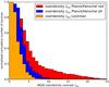 |
Fig. D.1
Cumulative histogram of the normalized overdensity contrast δ350 using the AKDE density estimator. Blue represents all our SPIRE sources, red represents only redder SPIRE sources, defined by S350/S250> 0.7 and S500/S350> 0.6, and orange 500 random fields in Lockman. Most of our fields show overdensities larger than 5. See Sect. 4.2 for details. |
| Open with DEXTER | |
Appendix E: Gallery of selected sources
We provide 3-colour images for a few sources drawn from the 228 of our sample. Each plot shows:
-
a 3-colour image of the SPIRE data, with 250μm in blue, 350μm ingreen, and 350μm in red (using the python APLpy module:show_rgb);
-
the Planck contour (IN region, i.e., 50% of the peak) as a bold white line;
-
the significance of the SPIRE overdensity contrast (starting at 2σ, and then incrementing by 1σ) as yellow solid lines.
Figure E.2 summarizes the 228 SPIRE sample.
 |
Fig. E.1
Representative Planck targets, showing 3-colour SPIRE images: blue, 250μm; green, 350μm; and red, 500μm. The white contours show the Planck IN region, while the yellow contours are the significance of the overdensity of 350μm sources, plotted 2σ, 3σ, 4σ, etc. |
| Open with DEXTER | |
 |
Fig. E.1
continued. |
| Open with DEXTER | |
 |
Fig. E.1
continued. |
| Open with DEXTER | |
 |
Fig. E.1
continued. |
| Open with DEXTER | |
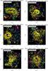 |
Fig. E.1
continued. |
| Open with DEXTER | |
 |
Fig. E.1
continued. |
| Open with DEXTER | |
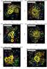 |
Fig. E.1
continued. |
| Open with DEXTER | |
 |
Fig. E.2
Mosaic showing the 228 SPIRE fields. |
| Open with DEXTER | |
© ESO, 2015
Current usage metrics show cumulative count of Article Views (full-text article views including HTML views, PDF and ePub downloads, according to the available data) and Abstracts Views on Vision4Press platform.
Data correspond to usage on the plateform after 2015. The current usage metrics is available 48-96 hours after online publication and is updated daily on week days.
Initial download of the metrics may take a while.